Virtual design software for mechanical system dynamics using transfer matrix method of multibody system and its application

Abstract

The complex mechanical systems such as high-speed trains, multiple launch rocket system, self-propelled artillery, and industrial robots are becoming increasingly larger in scale and more complicated in structure. Designing these products often requires complex model design, multibody system dynamics calculation, and analysis of large amounts of data repeatedly. In recent 20 years, the transfer matrix method of multibody system has been widely applied in engineering fields and welcomed at home and in abroad for the following features: without global dynamic equations of the system, low orders of involved system matrices, high computational efficiency, and high programming. In order to realize the rapid and visual simulation for complex mechanical system virtual design using transfer matrix method of multibody system, a virtual design software named MSTMMSim is designed and implemented. In the MSTMMSim, the transfer matrix method of multibody system is used as the solver for dynamic modeling and calculation; the Open CASCADE is used for solid geometry modeling. Various auxiliary analytical tools such as curve plot and animation display are provided in the post-processor to analyze and process the simulation results. Two numerical examples are given to verify the validity and accuracy of the software, and a multiple launch rocket system engineering example is given at the end of this article to show that the software provides a powerful platform for complex mechanical systems simulation and virtual design.

Introduction

With the development of technology of weapon, aeronautics, astronautics, vehicle, robot, and computer, numerous complex mechanical systems consisted of many bodies connected by various joints with one another have appeared to be considered as multibody systems (MSs). The methods of MS dynamics with different styles, such as Wittenburg method, Schiehlen method, and Kane method, developed rapidly in the last 40 years and made a great contribution to modern science and technology.^1,2

At present, commercial and free MS dynamic simulation software are mainly ADAMS, RecurDyn, MBDyn, Simpack, OpenModelica, and so on. These software usually consist of three parts: pre-processor, multibody dynamic solver, and post-processor. The solver is the core of MS dynamic simulation software, which is used to establish the system dynamic equations and to achieve the numerical solution. There are many methods to generate the dynamic equations. Wittenburg introduced graph theory into MS dynamics, which laid the foundation for automatically generating multibody dynamic equations using the Lagrangian method; Kane proposed Kane method which has characteristics of both structural mechanics and analytical mechanics, which applied the method in the application of spacecraft dynamics. In general, for these traditional methods, it is necessary to develop the global dynamic equations of the system. If the system structure is changed, the corresponding global dynamic equations must be deduced again. The orders of involved system matrices increase with the increase in the number of the degrees of freedom of the system, hence the orders of the matrices involved in the global dynamic equations are rather high for the complex MS. This is the main reason for the difficulties in calculating the complex mechanical system dynamics.

The transfer matrix method (TMM) was developed for a long time and used widely in structure mechanics and rotor dynamics of the linear time-invariant system. Holzer ³ initially applied TMM to solve the problems of torsion vibrations of rods. Dokanish ⁴ developed the finite element TMM to solve the problems of plate structure vibration analysis. Horner and Pilkey ⁵ proposed the Riccati TMM to circumvent the numerical stability of the boundary value problem.

Rui and Lu^6,7 studied the vibrations and orthogonality of the special linear MS by developing new transfer matrices. Rui et al.^8,9 developed the discrete time transfer matrix method of the multibody system (MS-DT-TMM) to study general multi-rigid-body system dynamics by combining and expanding the TMM and the numerical integration procedure. Rui ¹⁰ extended MS-DT-TMM to study dynamics of multi-rigid-flexible-body system moving in plane.^8,11–13 The MSTMM has been widely used in the national economy, defense industry, and other fields due to its following advantages: without the global dynamic equations of the system, low order of involved system matrix, fast computational speed, and high automation in programming. In order to use the MSTMM for the rapid calculation and virtual design of the mechanical system dynamics, the virtual design software for mechanical system dynamics using the MSTMM needs to be urgently developed.

Comments on commercial and free MS dynamic software

Comments on commercial MS dynamic software

General commercial MS dynamic simulation software, such as ADAMS, ¹⁴ RecurDyn, ¹⁵ and Simpack, ¹⁶ typically consists of a mature pre-processor for modeling MSs, MS dynamic solver, and post-processor for animation and curve plotting output. These commercial MS dynamic software with powerful functions provide not only general MS dynamic calculation module but also a variety of simulation modules for special industry applications. These commercial software provide a large number of project cases and powerful commercial technical support, which makes it easy and convenient for the users to learn and use. However, the commercial MS dynamic software obviously has some common shortcomings: (1) a copy of the commercial software for multibody dynamics is usually sold several hundreds of thousands of dollars, which is very expensive for some researchers or enterprises. (2) Users cannot get the source code from the commercial software, and the researchers may not know its internal working principle. Therefore, it is very hard for the users to modify the source code to improve the software.

Comments on free source MS dynamic software

As for free MS dynamic software, many universities and research institutes have had in-depth study for many years, such as Open Dynamic Engine (ODE), MBDyn, ¹⁷ MBS3D, OpenModelica, ¹⁸ EasyDyn, ¹⁹ HOTINT, ²⁰ and so on. Compared with mature commercial software, these software have many deficiencies, mainly reflected as follows: first, a lack of visual, interactive user interface brings the inconvenience for the engineers in designing and simulating, and, second, lack of a variety of model libraries and technical supports makes some software quite difficult to use. Nevertheless, the advantages of free software are obvious: first, there is no need to pay high copyright charge since most free software is based on the general public license (GPL) copyright license and free to use and modify; second, the free software is convenient for researchers to study the calculation process of MS dynamics deeply, including the software architecture, how to build dynamic equations from dynamic models, how to solve the dynamic equations, and so on; and third, users can modify the source code to meet the calculation needs for various projects through secondary development. Free MS dynamic software provides development ideas, architecture, and routes for reference to design virtual design software for mechanical system dynamics based on transfer matrix method of multibody system (MSTMM).

Theorems of MSTMM

The classical TMM has been developed over 70 years and was used widely in structure mechanics and rotor dynamics of linear time-invariant system. To linear system, Myklestad ²¹ applied TMM to determine the bending-torsion modes of beams, Thomson ²² applied TMM to more general vibration problems, Pestel and Leckie ²³ listed transfer matrices for elasto-mechanical elements up to 12th order, and Rubin^24,25 provided a general treatment for transfer matrices and their relation to other forms of frequency response matrices. Transfer matrices have been applied to a wide variety of engineering programs by a number of researchers, including Targoff, ²⁶ Lin, ²⁷ Lin and McDaniel, ²⁸ Mercer and Seavey, ²⁹ Mead and Gupta, ³⁰ Mead, ³¹ Henderson and McDaniel, ³² McDaniel, ³³ McDaniel and Logan, ³⁴ Murthy and colleagues,^35–37 and Ohga and Shigematus ³⁸ dealing with beams, beam-type periodic structures, skin-stringer panels, rib-skin structures, curved mutispan structures, cylindrical shells, stiffened rings, and so on. Dokanish ⁴ developed finite element TMM to solve the problems of plate structure vibration analysis, by combining finite element method and TMM. Many researchers, such as Ohga and Shigematus, ³⁸ Xue, ³⁹ and Loewy and colleagues,^40,41 studied and improved the finite element transfer matrix for structure dynamics. Horner and Pilkey ⁵ proposed Riccati TMM in order to circumvent the numerical stability of the boundary value problem. To date, Riccati transform is also an important tool to overcome the ill condition of the TMM.

Kumar and Sankar ⁴² developed DT-TMM for structure dynamics of time-variant system by combining the TMM with the numerical integration procedure. DT-TMM gives an important clue for dynamics of time-variant system. Rui et al. ¹² developed MSTMM for vibration analysis of linear MS by developing new transfer matrices and orthogonal property of MS. MSTMM provides an important thought that MS dynamics may be solved using TMM. The general idea of the MSTMM is as follows: first of all, break up a complicated system into component parts with dynamic properties that can be expressed in matrix form. These component matrices are considered as building blocks, when fitted together according to a predetermined library of the transfer matrices, and used to assemble the system. For the chain system, only successive matrix multiplications are necessary elements to fit together. Thus, the overall transfer matrix and the transfer matrix equation are obtained.^43,44 Rui et al. developed MS-DT-TMM to study general multi-rigid-body system dynamics by combining and expanding the TMM and the numerical integration procedure. The corresponding flowchart of algorithms for MS-DT-TMM is shown in Figure 1.

Figure 1.

Flowchart of algorithms for MS-DT-TMM.

State vectors

In order to describe conveniently, the chain MS is taken as an example in the following. The state vectors of the connection point among any rigid bodies and hinges moving in space are defined as

$$\mathit{z}={\left[\begin{array}{ccccccccccccc}\hfill x\hfill & \hfill y\hfill & \hfill z\hfill & \hfill {\theta }_x\hfill & \hfill {\theta }_y\hfill & \hfill {\theta }_z\hfill & \hfill m_x\hfill & \hfill m_y\hfill & \hfill m_z\hfill & \hfill q_x\hfill & \hfill q_y\hfill & \hfill q_z\hfill & \hfill 1\hfill \end{array}\right]}^T$$

(1)

where $x$ , $y$ , and $z$ are the position coordinates of the connection point with respect to the inertial reference system; ${\theta }_x,{\theta }_y,\mathrm{and}{\theta }_z$ are the corresponding orientation angles rotating in the directions of $x$ , $y$ , and $z$ ; $m_x,m_y,m_z,q_x,q_y,\mathrm{and}{q}_z$ are the corresponding internal torques and internal forces in the same reference system, respectively.

Linearization of dynamic equations of elements

According to numerical integration procedures, the motion parameters of MS $\stackrel{··}{\xi }$ (acceleration or angular acceleration) and $\stackrel{·}{\xi }$ (velocity or angular velocity) at the time instant $t_i$ are expressed as the linear function of $\xi$ (positions or rotation angles) as follows

$$\stackrel{··}{\xi }\left(t_i\right)=A\left(t_{i-1}\right)\stackrel{·}{\xi }\left(t_i\right)+B_x\left(t_{i-1}\right)$$

(2)

$$\stackrel{·}{\xi }\left(t_i\right)=C\left(t_{i-1}\right)\xi \left(t_i\right)+D_x\left(t_{i-1}\right)$$

(3)

where the variable $\xi$ may represent column matrix of the position coordinates $x$ , $y$ , and $z$ or the orientation angles ${\theta }_x,{\theta }_y,\mathrm{and}{\theta }_z$ , respectively; $\stackrel{··}{\xi }$ and $\stackrel{·}{\xi }$ represent the second- and first-order derivatives of $\xi$ with respect to time, respectively, that is, corresponding column matrices of acceleration and velocity or corresponding column matrices of angular acceleration and angular velocity, at the same time instant $t_i$ . The quantities, $B_x$ , $C$ , and $D_x$ , will have different expressions for different numerical integration procedures. There are many accurate and commonly available numerical integration procedures, such as For-Euler method, Newmark-β method, Wilson-θ method, and Houbolt method. For example, if Newmark-β method is used, then we obtain

$$\begin{array}{cc}\multicolumn{1}{c}{}& A=\frac{1}{\beta \mathrm{\Delta }{T}^2}\hfill \\ \multicolumn{1}{c}{}& C=\frac{\gamma }{\beta \mathrm{\Delta }T}\hfill \\ \multicolumn{1}{c}{}& B_x=A[-\xi \left(t_{i-1}\right)-\stackrel{·}{\xi }\left(t_{i-1}\right)\mathrm{\Delta }T-(\frac{1}{2}-\beta )\stackrel{··}{\xi }\left(t_{i-1}\right)\mathrm{\Delta }{T}^2]\hfill \\ \multicolumn{1}{c}{}& D_x=\stackrel{·}{\xi }\left(t_{i-1}\right)+(1-\gamma )\stackrel{··}{\xi }\left(t_{i-1}\right)\mathrm{\Delta }T+\gamma B_x\mathrm{\Delta }T\hfill \end{array}$$

(4)

Transfer equations and transfer matrices of elements

The dynamic equations of the $j\mathrm{th}$ element that have been linearized using a numerical integration procedure can be assembled into a single transfer equation

$${\mathit{z}}_{j,j+1}\left(t_i\right)={\mathit{U}}_j\left(t_i\right){\mathit{z}}_{j,j-1}\left(t_i\right)$$

(5)

The transfer equation describes the mutual relationship between the state vectors at the two ends of the $j\mathrm{th}$ element and has the similar form in contrast with a general transfer equation used in MSTMM, DT-TMM, or TMM. The matrix ${\mathit{U}}_j(t_j)$ is the transfer matrix of the $j\mathrm{th}$ element. It is the function of the motion quantities ( $\mathit{z}(t_k)$ , $\stackrel{·}{\mathit{z}}(t_k)$ , and $\stackrel{··}{\mathit{z}}(t_k)$ , $k=i-1,i-2,\dots$ ) which are all known at time instant $t_i$ . Its order is always ( $13\times 13$ ) for the dynamics of chain multi-rigid-body system moving in space or ( $7\times 7$ ) for the dynamics of chain multi-rigid-body system moving in plane.

Transfer equation and transfer matrix of overall system

Using the same method used in MSTMM, DT-TMM, or TMM, the overall system transfer equation and transfer matrix $\mathit{U}$ , which describe the relationship of the state vectors at boundary ends of the system, can be assembled and calculated. That is

$${\mathit{z}}_{n,0}={\mathit{U}}_{\mathrm{all}}{\mathit{z}}_{1,0}$$

(6)

$${\mathit{U}}_{\mathrm{all}}={\mathit{U}}_n{\mathit{U}}_{n-1}\dots {\mathit{U}}_2{\mathit{U}}_1$$

(7)

For a chain system, the order of the overall transfer matrix of the system is equal to the order of the transfer matrix of the element, and it does not increase when the degrees of freedom of the system increase. Irrespective of the size of an MS, the highest order of the overall transfer matrix $\mathit{U}$ is the same with the order of the transfer matrix of single-body element. So, the matrices involved in the MS-DT-TMM are always small, which greatly reduce the computational time and the memory storage requirement.

Automatic deduction theorem of overall transfer equation

It can be verified that the transfer equations of a rigid body j with L input ends and one output end can be written as

$${\mathit{z}}_{j,O}={\mathit{U}}_{j,I_1}{\mathit{z}}_{j,I_1}+{\mathit{U}}_{j,I_2}{\mathit{z}}_{j,I_2}+\cdots +{\mathit{U}}_{j,I_L}{\mathit{z}}_{j,I_L}$$

(8)

The geometrical equation can be written in the form of

$${\mathit{H}}_j{\mathit{z}}_{j,I_1}={\mathit{H}}_{j,I_k}{\mathit{z}}_{j,I_k}(k=2,3,4,\dots ,L)$$

(9)

where ${\mathit{H}}_j$ is a constant matrix extracting displacement variables (including position coordinates and orientation angles) from a state vector when pre-multiplying ${\mathit{z}}_{j,I_1}$ , and ${\mathit{H}}_{j,I_k}$ is related to the position between the first input end and $k\mathrm{th}$ input end of body. The number of the geometrical equations is $(L-1)$ .

The automatic deduction theorem of the overall transfer equation of multi-rigid-flexible-body systems has been verified ⁴⁵ as follows:

1. The state vectors involved in an overall transfer equation are the column matrix comprising the state vectors of all boundary ends of the system.

2. For a tree system, in the first line of the overall transfer matrix, the coefficient matrix of the state vector of root is a minus unit matrix, while each coefficient matrix of the state vector of a tip is the successive pre-multiplication of the transfer matrices of all elements in the transfer path from this tip to the root. Besides the first line in the overall transfer matrix, all coefficient matrices of state vectors in the first column are zero matrices. Except the first line, in each row, each nonzero partitioned matrix corresponds to the coefficient matrix of the tip state vector, from which there is a transfer path to the input end of the element with multiple input ends. Each nonzero coefficient matrix of the state vector of a tip is the successive pre-multiplication of all transfer matrices of elements in the transfer path from this tip to the kth input end ${\mathit{I}}_k$ of $j\mathrm{th}$ body element, which has more than two ends, then pre-multiplied by $-{\mathit{H}}_j$ four $k=1$ or pre-multiplied by ${\mathit{H}}_{j,I_k}$ ( $k=2,3,4,\dots ,L$ ).

3. For a chain system, its overall transfer matrix is deduced automatically by successive pre-multiplication of the transfer matrices of all elements in the transfer path from the tip to the root of the system. In fact, any chain system can be considered as a special example of the tree system in the case with only two boundary ends, for more details, see Rui et al. ⁴⁵

Thus, the transfer equation of the closed-loop system can be deduced automatically as is achieved for the chain system (Figure 2)

$${\mathit{z}}_{1,0}={\mathit{U}}_{n-1}{\mathit{z}}_{n,0}$$

(10)

Figure 2.

Topology of a closed-loop system after “cutting” the hinge n.

Attention should be paid that the state vectors of a couple of “cutting points” are the same, namely

$${\mathit{z}}_{1,0}={\mathit{z}}_{n,0}$$

(11)

Then, the transfer equation (10) of the closed-loop system can be deduced automatically by handwriting and by computer

$${\mathit{U}}_{\mathrm{all}}{\mathit{z}}_{1,0}=0,{\mathit{U}}_{\mathrm{all}}=(1-{\mathit{U}}_{n-1})$$

(12)

• 4. For a closed-loop system, its overall transfer equation is deduced automatically as the chain system, after treating the original system as the chain system by “cutting” a junction of any two adjacent elements and letting the couple of “cutting points” as the tip and root with the same state vectors of the chain system.

• 5. For a general system composed of one tree subsystem and some closed-loop subsystems, its overall transfer equation is deduced automatically as the tree system, after treating the original system as the tree system by “cutting” the junctions of any two adjacent elements in every closed-loop subsystem and letting every couple of “cutting points” as new “boundary ends” with the same state vectors of the tree system.

According to the automatic deduction theorem, the overall transfer equation of the tree system described in Figure 3 can be obtained readily

$${\mathit{U}}_{\mathrm{all}}{\mathit{z}}_{\mathrm{all}}=0$$

(13)

where

$$\begin{array}{cc}\multicolumn{1}{c}{}& {\mathit{U}}_{\mathrm{all}}=\left[\begin{array}{ccccc}\hfill -\mathit{I}\hfill & \hfill {\mathit{T}}_{15-1}\hfill & \hfill {\mathit{T}}_{16-1}\hfill & \hfill {\mathit{T}}_{17-1}\hfill & \hfill {\mathit{T}}_{18-1}\hfill \\ \multicolumn{1}{c}{\mathit{O}}& \hfill {\mathit{G}}_{15-9}\hfill & \hfill {\mathit{G}}_{16-9}\hfill & \hfill \mathit{O}\hfill & \hfill \mathit{O}\hfill \\ \multicolumn{1}{c}{\mathit{O}}& \hfill \mathit{O}\hfill & \hfill \mathit{O}\hfill & \hfill {\mathit{G}}_{17-10}\hfill & \hfill {\mathit{G}}_{18-10}\hfill \\ \multicolumn{1}{c}{\mathit{O}}& \hfill {\mathit{G}}_{15-4}\hfill & \hfill {\mathit{G}}_{16-4}\hfill & \hfill {\mathit{G}}_{17-4}\hfill & \hfill {\mathit{G}}_{18-4}\hfill \end{array}\right]\hfill \\ \multicolumn{1}{c}{}& {\mathit{z}}_{\mathrm{all}}=\left[\begin{array}{c}\hfill {\mathit{z}}_{1,0}\hfill \\ \multicolumn{1}{c}{{\mathit{z}}_{15,0}}\\ \multicolumn{1}{c}{{\mathit{z}}_{16,0}}\\ \multicolumn{1}{c}{{\mathit{z}}_{17,0}}\\ \multicolumn{1}{c}{{\mathit{z}}_{18,0}}\end{array}\right]\hfill \end{array}$$

(14)

$$\{\begin{array}{c}\hfill {\mathit{T}}_{15-1}={\mathit{U}}_1{\mathit{U}}_2{\mathit{U}}_3{\mathit{U}}_4{\mathit{U}}_5{\mathit{U}}_7{\mathit{U}}_8{\mathit{U}}_9{\mathit{U}}_{11}{\mathit{U}}_{15}\hfill \\ \multicolumn{1}{c}{{\mathit{T}}_{16-1}={\mathit{U}}_1{\mathit{U}}_2{\mathit{U}}_3{\mathit{U}}_4{\mathit{U}}_5{\mathit{U}}_7{\mathit{U}}_8{\mathit{U}}_{9,12}{\mathit{U}}_{12}{\mathit{U}}_{16}}\\ \multicolumn{1}{c}{{\mathit{T}}_{17-1}={\mathit{U}}_1{\mathit{U}}_2{\mathit{U}}_3{\mathit{U}}_{4,6}{\mathit{U}}_6{\mathit{U}}_{10}{\mathit{U}}_{13}{\mathit{U}}_{17}}\\ \multicolumn{1}{c}{{\mathit{T}}_{18-1}={\mathit{U}}_1{\mathit{U}}_2{\mathit{U}}_3{\mathit{U}}_{4,6}{\mathit{U}}_6{\mathit{U}}_{10,14}{\mathit{U}}_{14}{\mathit{U}}_{18}}\end{array}$$

(15)

$$\begin{array}{cc}\multicolumn{1}{c}{}& \{\begin{array}{c}\hfill {\mathit{G}}_{15-9}=-{\mathit{H}}_9{\mathit{U}}_{11}{\mathit{U}}_{15}\hfill \\ \multicolumn{1}{c}{{\mathit{G}}_{16-9}={\mathit{H}}_{9,12}{\mathit{U}}_{12}{\mathit{U}}_{16}}\end{array}\hfill \\ \multicolumn{1}{c}{}& \{\begin{array}{c}\hfill {\mathit{G}}_{17-10}=-{\mathit{H}}_{10}{\mathit{U}}_{13}{\mathit{U}}_{17}\hfill \\ \multicolumn{1}{c}{{\mathit{G}}_{18-10}={\mathit{H}}_{10,14}{\mathit{U}}_{14}{\mathit{U}}_{18}}\end{array}\hfill \\ \multicolumn{1}{c}{}& \{\begin{array}{c}\hfill {\mathit{G}}_{15-4}=-{\mathit{H}}_4{\mathit{U}}_5{\mathit{U}}_7{\mathit{U}}_8{\mathit{U}}_9{\mathit{U}}_{11}{\mathit{U}}_{15}\hfill \\ \multicolumn{1}{c}{{\mathit{G}}_{16-4}=-{\mathit{H}}_4{\mathit{U}}_5{\mathit{U}}_7{\mathit{U}}_8{\mathit{U}}_{9,12}{\mathit{U}}_{12}{\mathit{U}}_{16}}\\ \multicolumn{1}{c}{{\mathit{G}}_{17-4}={\mathit{H}}_{4,6}{\mathit{U}}_6{\mathit{U}}_{10}{\mathit{U}}_{13}{\mathit{U}}_{17}}\\ \multicolumn{1}{c}{{\mathit{G}}_{18-4}={\mathit{H}}_{4,6}{\mathit{U}}_6{\mathit{U}}_{10,14}{\mathit{U}}_{14}{\mathit{U}}_{18}}\end{array}\hfill \end{array}$$

(16)

Figure 3.

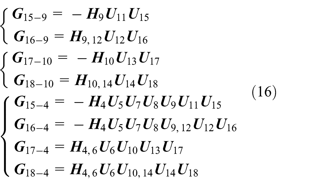
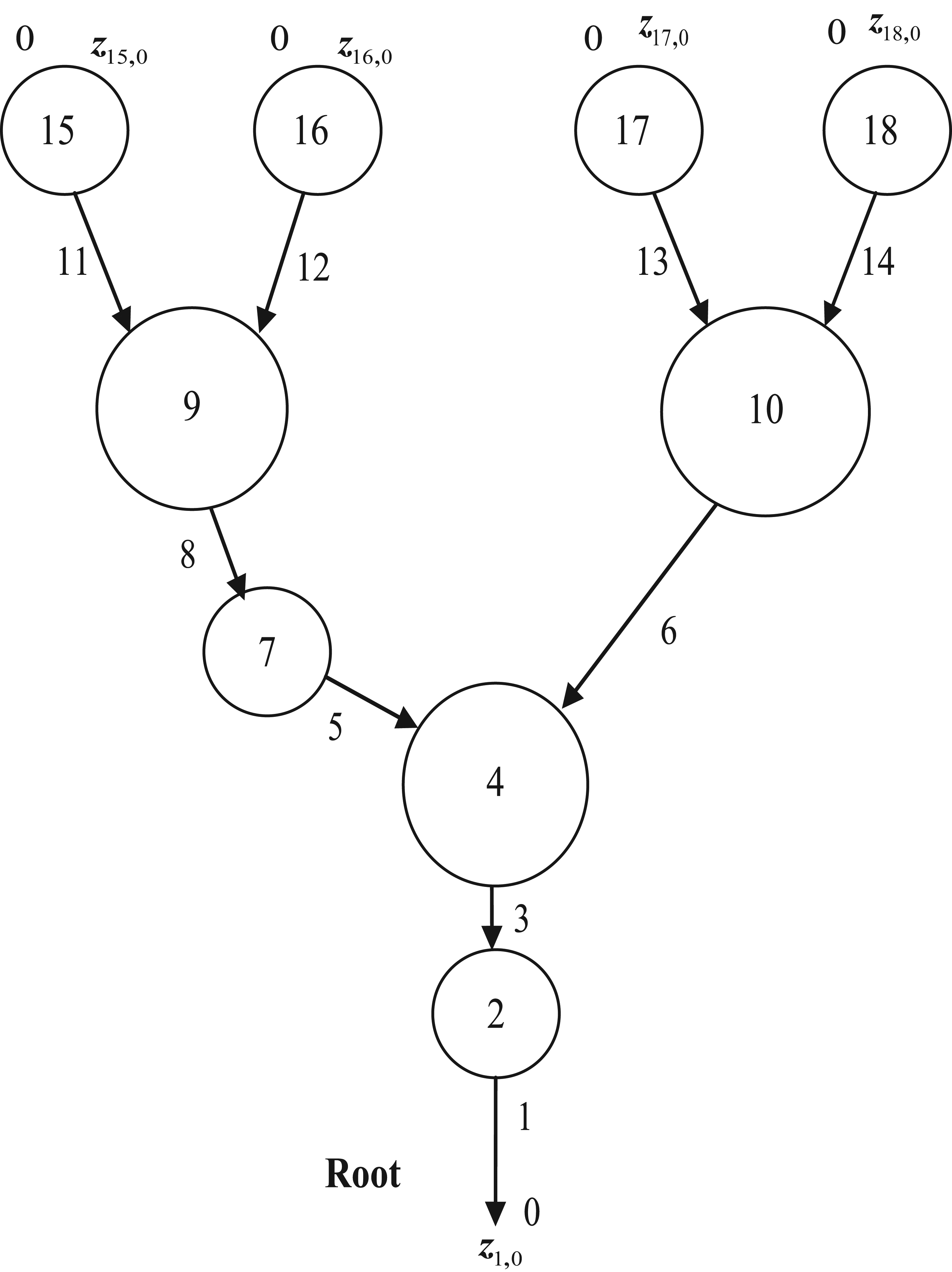
General multibody system processing to tree system.

Architecture of virtual design software for mechanical system dynamics based on the MSTMM

Functions and characteristics of MSTMMSim

1. According to the ideas of the user, the software can automatically generate the solid geometric figure of the object by human–computer interaction and show a three-dimensional (3D) view from different perspectives on the computer screen, including the shape, size, color, and the material of the object.

2. According to the solid geometric figure of the object, the software can automatically generate the corresponding parameters of the object, including mass, moment of inertia, and the center of mass.

3. According to the solid geometric figure of each object, the software can automatically assemble these components into a mechanical system and can automatically match the size parameters with the object to ensure that the components in the system do not interfere with each other.

4. Once the solid geometric figures and structural parameters of the mechanical system are defined, the software can automatically generate the multibody dynamic model and its topology structure diagram accordingly.

5. According to the 3D geometry of mechanical system, the software can automatically generate the dynamic parameters for the calculation of the dynamics of an MS.

6. The transfer matrices of different mechanical elements, such as bodies, joints, and control elements, are packed up as a library in the software. The transfer matrix library for MSs provides an important tool for setting up the large-scale dynamic simulation software with powerful functions and high computational speed.

7. According to the mechanical system topological structure, the software can automatically generate the transfer equation and transfer matrix of the element by calling the transfer matrix library and generate the overall transfer equation, overall transfer matrix, and boundary conditions of the system.

8. According to the needed parameters for dynamic calculation which are automatically generated by computer or manually input by users, the software can automatically and rapidly calculate the dynamics of the MS and return the calculation results.

9. The calculation results for multibody dynamics could be saved, displayed, and printed on the forms of data file, figure file, curve file, and animation file.

10. Virtual design for the dynamics of the mechanical system can be performed; scheme of virtual design for the dynamics of the mechanical system can be automatically built; the optimal design for the dynamics of a mechanical system can be performed.^46–48

Architecture design of MSTMMSim

The system architecture of MSTMMSim is shown in Figure 4. The architecture of MSTMMSim is based on the ideas of service-oriented architecture (SOA), which includes five layers:

1. Modeling and Display Service Layer. This layer provides a user interface for visual modeling and post-processing (simulation results data curve output, 3D model animation).

2. Data Store Service Layer. This layer provides a function for managing modeling and simulation results data, which integrates the interface of computer-aided design (CAD), geometric modeling, finite element, and the technology of database, XML.

3. Multibody Dynamic Solving Service Layer. This layer provides a solver for the MS dynamic calculation. The solver can be ADAMS, RecurDyn, MBDyn, or MSTMM, called according to the needs of the users.

4. Multibody Dynamic Solving Service Bus. This bus is used to invoke different MS dynamic solvers for different dynamic analyses according to analysis requirements. The simulation results are sent to Data Store Service Layer by this bus.

5. Data Service Bus. This bus is used for passing the modeling and simulation results data between Modeling and Display Service Layer and Data Store Service Layer.

Figure 4.

Architecture of MSTMMSim.

The basic module of MSTMMSim is based on MSTMM, which consists of three parts: the pre-processor, MSTMM solver, and post-processor. The software and the graphical user interface (GUI) are developed by C++ language and QT framework, respectively. QT is a cross-platform C++ application development framework developed by Nokia, which is widely used in the development of GUI programs. The software integrates Open CASCADE (OCC)^49,50 geometric modeling kernel library, so that the user can import various types of CAD solid models to the software. The software calls the application programming interface (API) of OCC to achieve basic geometry modeling. It can also achieve complex geometric model design rapidly by the so-called union, difference, and intersection of Boolean operation. The software automatically generates the topology structure and parameters of the mechanical system dynamics by the definition of user on GUI. ⁵¹ The software reads the defined parameters, calculates system dynamics, stores the results data, returns the results to the user in the form of animation and curves. The workflow of the software is shown in Figure 5.

Figure 5.

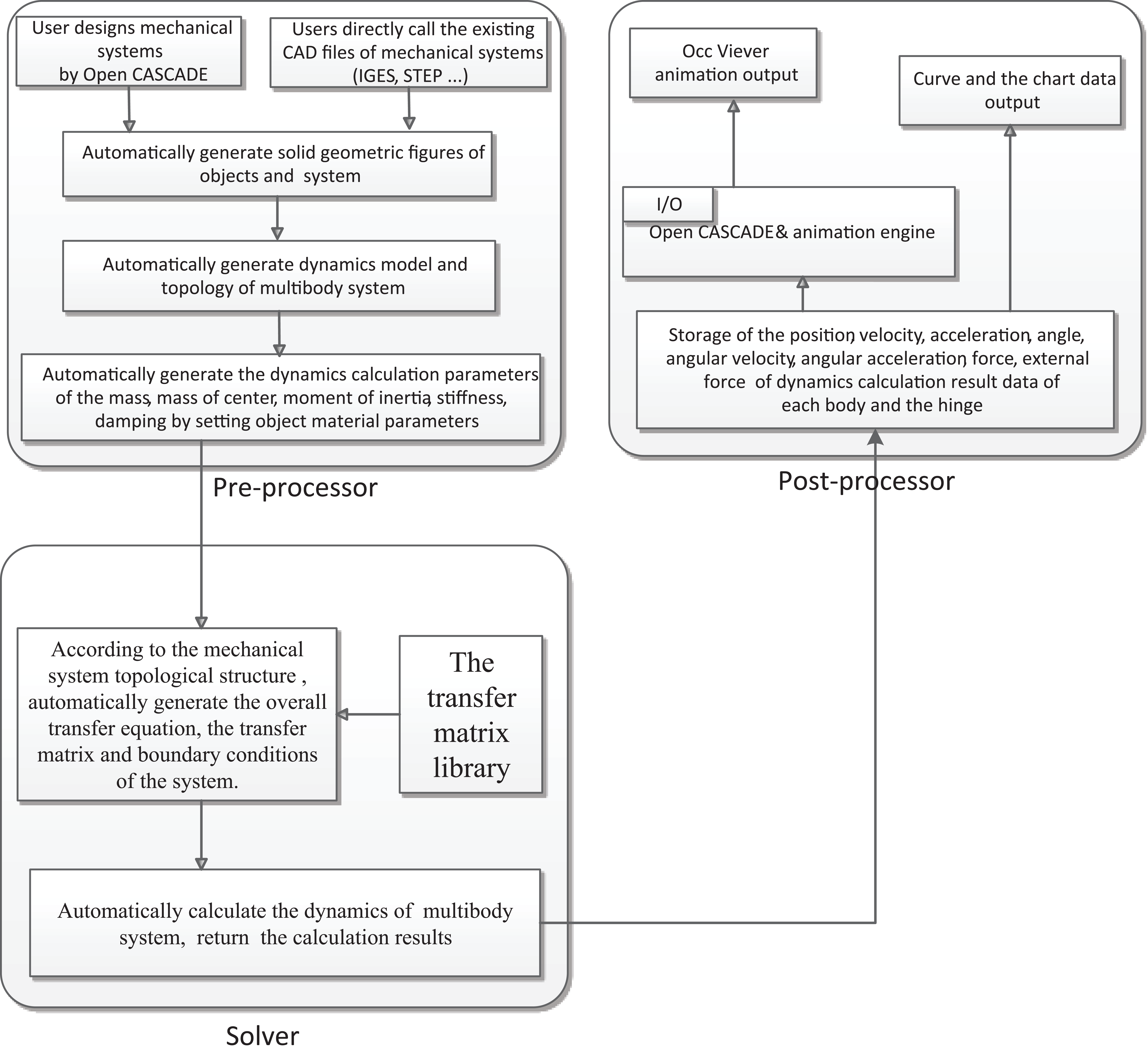
Workflow of the MSTMMSim.

According to the viewpoint of design of software and component thinking, the software can be divided into six components: “User Interface,”“QT,”“Open CASCADE,”“Simulation,”“Rendering,” and “App.”Figure 6 shows the main class component of the MSTMMSim:

1. QT: GUI component

2. Qt_Gui: provides user interface (includes menu, button, dialog, etc.), which inherits the GUI class of QT;

3. Qt_OpenGL: provides rendering service based on Open Inventer.

Rendering: 3D rendering service component

Rd_OpenGL: provides 3D rendering services, which inherits the class of OpenGL;

Rd_Coin3D: provides management of OpenGL pipeline, scene object structure, model-view conversion, and rendering state, which inherits the class of Coin3D.

Simulation: MS dynamic calculate component

Si_MSTMMSimSolver: provides solving service of MS dynamics based on MSTMM and calculates the dynamics of MS;

Si_MBModel: provides MS model storage service, used for 3D solid and dynamic model of MS storage management;

Si_SimDate: provides storage of the simulation result management service.

User interface: visualization service component

Ui_Editor: provides establishment of service of dynamics and geometry model of mechanical system, which is realized by calling QT and OCC;

Ui_Viewer: provides 3D graphics display and animation service, which is implemented by calling the service of Occ_Viewer.

OCC: 3D solid geometric modeling components

Occ_Viewer: provides 3D display view service, which is rendered by calling “Rendering” component;

Occ_Shape: provides basic 3D solid geometry model modeling service (includes box, cylinder, ball, etc.), which is implemented by calling the API of OCC;

Occ_Geom: provides geometry parameters computing service (such as the length of edge, area of the surface, and volume of body), which inherits the basic class of geometric object of OCC;

Occ_ModelIO: provides service of read and storage of CAD files, which is implemented by inheriting the data exchange class of OCC.

App: the entrance and initialization of the software

Main: provides start and initializes the software (includes configure environment variable, initialize several of parameters, etc.);

Base: provides several classes of foundation library (such as matrix operations, numerical integration, and XML parsing).

Figure 6.

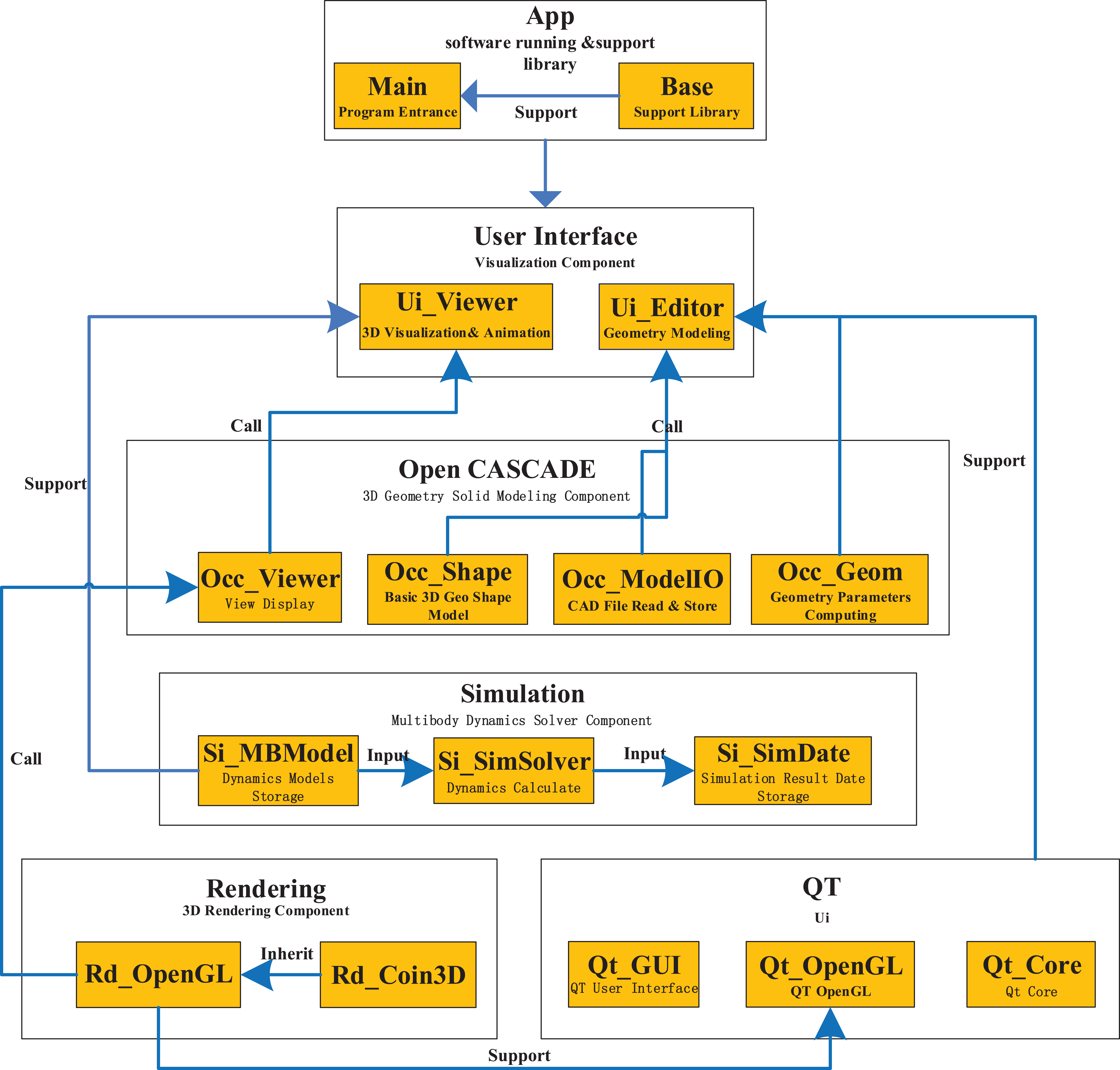
Main class component of the MSTMMSim.

The users can design the mechanical system via pre-processor module provided by OCC geometric modeling kernel; they can also import standard format CAD files, such as IGES, STEP, DWG/DXF, and so on, generated by other CAD software into MSTMMSim. Thereby, the software can generate the solid geometric figures of the mechanical system. Once the solid geometric figures are obtained, by setting the parameters of material properties, the software can automatically calculate the mass, center of mass, and moment of inertia, respectively, and automatically generate the parameters of the multibody model required by the dynamic calculation.

According to the parameters of the MS, the MSTMM solver calls the transfer matrix library, obtains the transfer equation and transfer matrix of each element, and automatically generates the overall transfer equation and overall transfer matrix of the system. The solver finally uses step-by-step time integration method for dynamic calculations.

The post-processor is mainly responsible for storing the calculated result data from the solver, including the position, velocity, acceleration, angle, angular velocity, and so on, of each body and joint. The data output is achieved by means of animation and curve plotting. The modules of MSTMMSim are given in Table 1.

Table 1.

Modules of MSTMMSim.

Basic modules	Sub-modules
Pre-processor	Parametric CAD geometry solid modeling module based on Open CASCADE
	CAD file import and export modules
	Object structure parameters automatic generation module
	Multibody system dynamic parameters automatic generation module
	Multibody system dynamic model and topology structure definition file automatic generation module
MSTMM solver	Transfer matrix library
	Input file parser module
	Transfer equation and transfer matrix of element, overall transfer equation, overall transfer matrix, and boundary conditions of the system automatic generation module
	Numerical calculation module for MSTMM
Post-processor	Calculation result data storage module
	Animation output module
	Curve and chart output module

CAD: computer-aided design; MSTMM: transfer matrix method of multibody system.

Design of the pre-processor module

OCC is an open source CAD or computer-aided manufacturing (CAM) or computer-aided engineering (CAE) geometric modeling kernel library developed by a French company, Matra Datavision. The OCC provides a C++ class library for drawing two-dimensional (2D) and 3D geometric figures, a large number of APIs for generating 2D or 3D solid geometric models, and integrates OpenGL display engine for rendering. The user can create 3D geometric model, import or export various types of CAD files, carry on Boolean operation (union, difference, and intersection), render the geometric model on the screen, and so on. The OCC provides a very convenient geometric modeling and 3D display environment for the development of visual simulation software of MS.

The pre-processor module of the software uses an interactive GUI provided by QT. The multiple document interface (MDI) of QT is responsible for the management of running environment and internal control, making visual simulation processing with good human–computer interaction. The user interface is shown in Figure 7.

Figure 7.

User interface of MSTMMSim.

In this article, the OCC geometric kernel provides 3D modeling, Boolean geometry operation, views, and data management to process 2D or 3D modeling problems. Through the OCC geometric modeling library, the software provides a virtual 3D geometric modeling platform for MS dynamic simulation.

Typically, a MS is composed of many bodies and joints, in which the bodies may be rigid or flexible body. In this article, only the rigid body is considered (in geometry, it can be described as box, cylinder, sphere, etc.); the joints in MSTMM have many types, such as ball-and-socket hinge, smooth hinge, elastic-damping hinge, and so on. When calculating Multibody System dynamics by computers, the dynamics parameters needs to input into the software. The parameters of body include ID, mass, geometry, center of mass, moment of inertia and the orientation coordinates of the body. The parameters of joint contain ID, type and ID of the adjacent rigid body by the joint. Some parameters can be obtained from CAD files, such as mass, geometry, center of mass, and moment of inertia. Other parameters (joint and body connecting relationships, position, and orientation of bodies) can be obtained from assembly relationships from the CAD files.

In order to obtain these parameters, the MSTMMSim calls the API of the OCC to extract the related parameters directly from the CAD models. Other parameters of the bodies and joints in the assembly space and geometric topology need some relevant calculation. Extracted associated parameters directly from the CAD assembly model could make the design model and the computational model consistent.

Design of 3D geometric and dynamic model

In order to define the geometry of a rigid body, the software calls the API of OCC implemented by GUI, such as defining a sphere, as shown in Figure 8:

BRepPrimAPI_MakeSphere mkSphere(gp_Ax2(p,d), radius, angle1, angle2, angle3);

TopoDS_Shape shape = mkSphere.Shape().

Figure 8.

Establish body model.

In order to obtain the parameters of rigid bodies directly from the CAD models, such as mass, center of mass, and moment of inertia, the software directly obtains them from the class of GProp_GProps in the OCC:

1. Obtain mass

   double TopoShapeSolid::getMass(void) const

   {

   GProp_GProps props;

     BRepGProp::VolumeProper ties(getTopoShapePtr()->_Shape, props);

     double c = props.Mass();

     return c;

   }

2. Obtain center of mass

   Vector3 TopoShapeSolid::getCenterOfMass(void) const

   {

     GProp_GProps props;

   BRepGProp::VolumeProperties(getTopoShapePtr()->_Shape, props);

     gp_Pnt c = props.CentreOfMass();

     return Vector3d(c.X(),c.Y(),c.Z());

   }

3. Obtain moment of inertia

   Matrix4D TopoShapeSolid::getMatrixOfInertia (void) const{

      GProp_GProps props;

   BRepGProp::VolumeProperties(getTopoShape Ptr()->_Shape, props);

      gp_Mat m = props.MatrixOfInertia();

      Base::Matrix4D mat;

      for (int i = 0; i < 3; i++) {

        for (int j = 0; j < 3; j++) {

          mat[i][j] = m(i + 1,j + 1);

        }

      }

      return mat;

   }

Design of joints

The parameters of different types of joints are different. For example, to define the parameters of a revolute hinge, the users need to define ID of the joint, ID of the rigid body connected to the joint, relative offset, and relative axis orientation of the joint in the reference frame respective to the connected bodies. This is shown in Figure 9.

Figure 9.

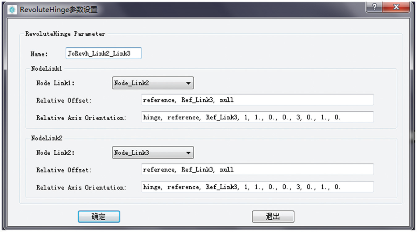
Definitions of spherical hinge.

Parameter definition file of MS dynamics

The defined parameters need to be stored in the computer system for subsequent calculation. On the basis of studying the parameter definition file storage structure of ADAMS, MBDyn, RecurDyn, and other MS dynamic software, and taking scalability and compatibility of the file into consideration, this article presents an XML-based parameter definition file format for storing the parameters for MS dynamic simulation. The following codes show a two-pendulum system composed of three rigid bodies connected by a “revolute pin” and a “revolute hinge” under the effect of gravity:

<model>

<model name>

<name>2-pendumul</name>

<path>C:\penduml2.step</path>

</model name>

<initial value>

<initial time>0</initial time>

<final time>5.</final time>

<time step>1.e-3</time step>

</initial value>

<controldata>

<structuralnodes>2</structuralnodes>

<rigidodies>2</rigidbodies>

<joints>2</joints>

<gravity>0., 0., -1., const, 9.81</gravity>

</controldata>

<parameters>

<parameter>

<name>M</name>

<type>real</type>

<value>1</value>

</parameter>

...

</parameters>

<nodes>

<structural>

<name>Node_Link1</name>

<type>dynamic</type>

<absoluteposition>1./2.*L, 0., 0.</absoluteposition>

<absoluteorientation>1,1,1</absoluteorientation>

<absolutevelocity>null</absolutevelocity>

<absoluteangularvelocity>null</absoluteangularvelocity>

</structural>

<structural>

<name>Node_Link2</name>

<type>dynamic</type>

<absoluteposition>1./2.*L, 0., 0.</absoluteposition>

<absoluteorientation>1,1,1</absoluteorientation>

<absolutevelocity>null</absolutevelocity>

<absoluteangularvelocity>null</absoluteangularvelocity>

</structural>

<elements>

 <bodies>

 <body>

 <name>Body_Link1</name>

 <node>Node_Link1</node>

 <mass>M</mass>

 <relativecentermass>null</relativecentermass>

 <inertiamatrix>diag, 0., M*L^2./12., M*L^2./12.</inertiamatrix>

 </body>

 <body>

 <name>Body_Link2</name>

 <node>Node_Link2</node>

 <mass>M</mass>

 <relativecentermass>null</relativecentermass>

 <inertiamatrix>diag, 0., M*L^2./12., M*L^2./12.</inertiamatrix>

 </body>

 <bodies>

      ...

<joints>

 <revolutepin>

<name>JoRevp_Link1</name>

<node>Node_Link1</node>

<relativeoffset>-1./2.*L, 0., 0.</relativeoffset>

<relativeaxisorientation>hinge, 1, 1., 0., 0., 3, 0., 1., 0.</relativeaxisorientation>

<absoluteoffset>null</absoluteoffset>

<absoluteaxisorientation>hinge, 1, 1., 0., 0., 3, 0., 1., 0.</absoluteaxisorientation>

</revolutepin>

<revolutehinge>

<name>JoRevh_Link1_Link2</name>

<node1>

<name>Node_Link1</name>

<relativeoffset>1./2.*L, 0., 0.</relativeoffset>

<relativeaxisorientation>hinge, 1, 1., 0., 0., 3, 0., 1., 0.</relativeaxisorientation>

</node1>

<node2>

<name>Node_Link2</name>

<relativeoffset>-1./2.*L, 0., 0., </relativeoffset>

<relativeaxisorientation>hinge, 1, 1., 0., 0., 3, 0., 1., 0.</relativeaxisorientation>

</node2>

</revolutehinge>

</joints>

</elements>

</model>

Because there are many mature solutions for parsing XML, such as tinyxml, xmlite, libxml, and so on, and the structured and standardized XML file has the advantage of high storage efficiency and readability, it can be very intuitive to describe MS dynamic topology and parameters of each element by defining these XML files.

Design of the solver module

The solver is the core of the software, which is responsible for all the calculations involved in the simulation software, such as automatically generating dynamic equations of the mechanical system and solving the numerical solution. The most important part of the solver is the algorithm of the MS dynamics. MSTMM is suitable for time-varying, nonlinear, large motion, and controlled general MS; the algorithm to compute the multi-rigid-body system dynamics on the computer using the MSTMM is as follows:^52–55

1. Determine the initial conditions and the boundary conditions of the system and set $i=1$ .

2. Compute the coefficients $A$ , $B_z$ (or ${\mathit{B}}_{\mathit{z}}$ ), $C$ , $D_z$ (or ${\mathit{D}}_{\mathit{z}}$ ), $\mathit{A}$ , $\mathit{\Phi }$ , ${\mathit{T}}_1$ , ${\mathit{T}}_2$ , ${\mathit{T}}_3$ , $\overline{s}$ , $\overline{c}$ , and so on at time $t_i$ for each connecting element by the linearization method and determine the initial conditions $z(t_{i-1})$ , $\stackrel{·}{z}(t_{i-1})$ , and $\stackrel{··}{z}(t_{i-1})$ at time $t_i$ as well as the system parameters.

3. Formulate the transfer matrix for each subsystem and the overall transfer matrix at time $t_i$ , respectively.

4. Apply the boundary conditions and the overall transfer equation to compute the unknown quantities in the boundary state vectors at time $t_i$ .

5. Using the transfer equations of each element, compute the state vectors of each element at time $t_i$ .

6. Use the state vectors at time $t_i$ to compute the first- and second-order derivatives of the position coordinates and rotation angles with respect to time $t_i$ .

7. Set $i=i+1$ , use the computational results of the last step as the initial conditions, and return to step 2, until the time required for a complete analysis.

In order to achieve kinematics and kinetics numerical analysis of the mechanical system, based on object-oriented thinking, using the theory of the MSTMM, this article designs and implements the solver for MSTMM-Si_MSTMMSimSolver. The class implementation is shown in Figure 10.

Figure 10.

Class diagram of solver of MSTMM.

MSTMM solver has good scalability by being divided into eight modules according to the solve processing and by decoupling the relationships among these modules using virtual interface (virtual function). ⁵⁶

1. InputFileParser: parser the parameter file. This class is responsible for parsing the parameter file defined in section “Parameter definition file of MS dynamics.” We use the tinyXML to parse the file, the solver reads the parameter file by the LoadFile() function of the tinyXML, parse the model parameter file by the Parser() to analyze the key value, such as the codes in section “Parameter definition file of MS dynamics” (<body> <name> Body_Link1 </name>... </body>). The “<body>” and “<name>” are key characters, and “Body_Link1” is the value. The parser constructs a structure of an array of strings—a key character table (Key Table) used to distinguish between keywords and data on the parameter file.

2. MbsModel: expression of MS models. The data are difficult to identify with the software after parsing from InputFileParser, and the model parameters need to correspond to the MS model. This process is called instantiation.

3. TransferMatrix: the library of MSTMM. This class includes the library of various types of transfer matrix of elements and outputs the transfer matrix of element by the type and parameters of the input.

4. MSTMMSFormulation: transfer equations and assemble transfer matrix. According to the expression of the MS models in MbsModel, this class calls the transfer matrix in the transfer matrix library, obtains the transfer matrix and transfer equation of the elements, and assembles the overall transfer matrix and overall transfer equation of the MS.

5. NumericalSolver: numerical solver. The class uses step-by-step time integration method for dynamic calculation.

6. MSTMMSimSolution: decider for simulation (extended). According to the user’s different needs, the class calls different solvers to calculate and outputs different results.

7. SimulationData: store the calculation results. The results will be stored by SimulationData class calculated by NumericalSolver class and can be stored in the form of database or file, and the software designed in this article currently only implementing storage in files; database storage method needs to be further developed.

8. MSTMMSimSolver: the interfaces of the MSTMM solver. MSTMMSimSolver is the interface of the solver. The solver could be regarded as a component exposed to an external function or program for calling as component service.

The software calls the solver using the threaded approach, which means the main program starts another thread to execute the solvers. The code is as follows:

this->dravecmd = new QProcess;

try{

QStringList arguments;

arguments<< ui->FileSelectEdit->text();

cmd->start(tr(“bin//transMultibbodySimCore.exe”), arguments);

}

catch (const Base::Exception& e) {

QMessageBox::information(this,tr(“error”),tr(“Sorry, Input File Error!”));

}

The simulation information as well as the debug message will output on the interface of the main window, as shown in Figure 11.

Figure 11.

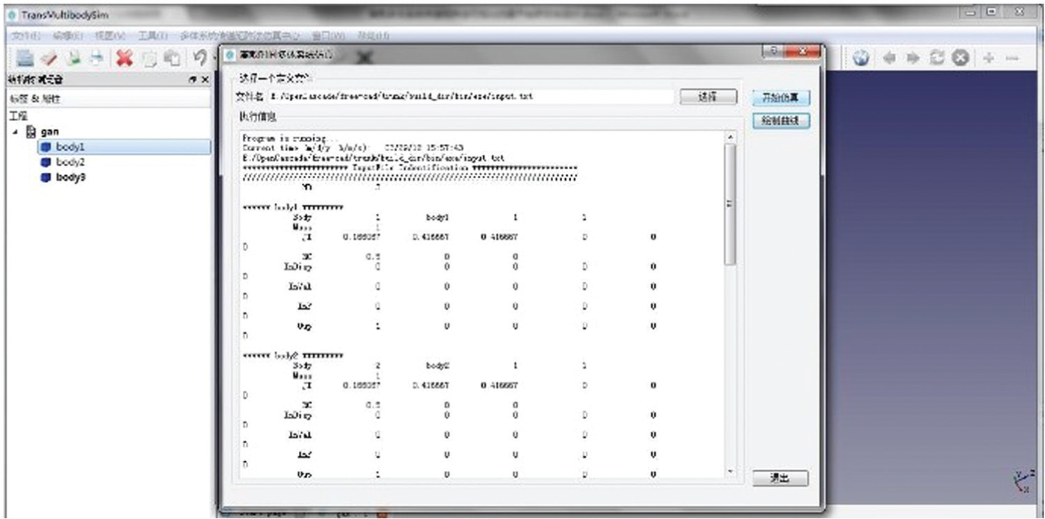
Solver calculation process output.

After finishing the calculation, the solver writes the result data to the result file, and the file storage format is shown in Table 2.

Table 2.

Simulation result storage format.

A		B	C	D	E	F	G	H	I	J	K	L	M	N	O
1	Time	No1–ang1	No1–ang2	No1–ang3	No2–ang1	No2–ang2	No2–ang3	No3–ang1	No3–ang2	No3–ang3	No1–acc1	No1–acc2	No1–acc3	No2–acc1	No2–acc2
2	0	0	0	0	0	0	0	0	0	0	0	0	0	0	0
3	0.1	1.02E−08	−6.58E−07	−0.05388	1.10E−08	7.27E−06	0.005341	−3.87E−06	0.009982	−0.00059	7.07E−07	−3.24E−05	−1.07467	7.44E−07	0.00036
4	0.2	1.13E−06	−1.78E−05	−0.21153	5.79E−07	0.000212	0.015051	−1.31E−05	0.019451	−0.0013	3.63E−05	−0.000388	−2.03672	5.49E−06	0.004956
5	0.3	1.20E−05	−7.61E−05	−0.44771	−2.19E−05	0.001247	−0.01084	0.0001014	0.026638	0.003381	0.000198	−0.000587	−2.60461	−0.00084	0.01654
6	0.4	3.40E−05	−4.79E−05	−0.71551	−0.000348	0.003545	−0.14152	0.0004449	0.029648	0.015393	0.000128	0.0018705	−2.6624	−0.00719	0.028918
7	0.5	−3.17E−06	0.0005273	−0.96057	−0.001847	0.006764	−0.42574	0.000202	0.027244	0.006598	−0.00113	0.0113373	−2.13776	−0.02472	0.03282
8	0.6	−0.0002255	0.0026459	−1.12991	−0.005401	0.009222	−0.85737	−0.002832	0.019194	−0.12792	−0.00336	0.0328806	−1.26892	−0.04417	0.01096
9	0.7	−0.0007793	0.0069278	−1.24814	−0.009536	0.008553	−1.30799	−0.008453	0.007404	−0.57188	−0.00941	0.0482279	−1.35801	−0.03177	−0.02084
10	0.8	−0.0025517	0.0110278	−1.43722	−0.011201	0.005743	−1.52685	−0.009032	−0.00449	−1.37836	−0.02719	0.0250123	−2.46533	−0.00392	−0.03556
11	0.9	−0.0054159	0.0101657	−1.69341	−0.011524	0.002182	−1.62296	−0.003442	−0.00586	−2.27028	−0.02393	−0.041076	−2.3539	−0.00463	−0.02744
12	1	−0.0069429	0.0039072	−1.89718	−0.011934	0.000888	−1.95614	−0.001524	0.000165	−2.83943	−0.00706	−0.078355	−1.80608	−0.00375	−0.00024
13	1.1	−0.0069005	−0.004089	−2.08374	−0.012367	0.001009	−2.39542	−0.00207	0.006692	−3.04814	0.008467	−0.074135	−2.07087	−0.00429	−0.00422
14	1.2	−0.0051093	−0.009885	−2.32518	−0.012518	−0.00076	−2.76235	−0.001617	0.011451	−3.0063	0.027114	−0.039389	−2.74309	0.002253	−0.03183
15	1.3	−0.0018258	−0.011939	−2.61755	−0.011986	−0.00505	−2.97693	−0.00021	0.012542	−2.89241	0.035761	−0.003284	−2.99538	0.006913	−0.05112
16	1.4	0.00148461	−0.011087	−2.90064	−0.011409	−0.01027	−3.05768	0.0007599	0.009362	−2.8077	0.028268	0.0168939	−2.5496	0.004142	−0.04983
17	1.5	0.00361638	−0.009149	−3.10924	−0.011058	−0.01467	−3.08599	0.001041	0.002949	−2.76607	0.014384	0.0201272	−1.57223	0.003735	−0.03847
18	1.6	0.00447298	−0.00717	−3.21209	−0.010558	−0.01828	−3.11612	0.0010241	−0.00462	−2.74183	0.003501	0.019649	−0.48821	0.006459	−0.0354
19	1.7	0.00446271	−0.005161	−3.20753	−0.00974	−0.02195	−3.1567	0.0008012	−0.01216	−2.71571	−0.003	0.0205227	0.580528	0.010072	−0.03793
20	1.8	0.00401509	−0.00324	−3.09589	−0.008557	−0.02548	−3.20637	0.0004042	−0.01972	−2.69034	−0.00532	0.0159232	1.64174	0.012781	−0.02877
21	1.9	0.00345351	−0.002507	−2.88655	−0.007647	−0.02672	−3.24096	0.0005626	−0.02798	−2.69552	−0.00622	−0.00364	2.48156	0.00173	0.008165
22	2	0.00260089	−0.004161	−2.61496	−0.008894	−0.02357	−3.1908	0.0029332	−0.03698	−2.76677	−0.01192	−0.02904	2.8639	−0.02852	0.053354

Design of post-processor module

The post-processor module of the software is very important for the simulation. ⁴⁸ The users can use the simulation results of observation and analysis to design mechanical systems. The post-processor includes dynamic curve plotting and 3D animation module to reflect the characteristics of the design model. The curve plotting module integrates open source Qwt (Qt widgets for technical applications) curve plotting package. The Qwt is an open source project based on the copyright based on LGPL, which provides a 2D plotting widget. The software reads the simulation data from the result file output to Qwt to achieve the curve plotting, as shown in Figure 12.

Figure 12.

Curve output module.

In research and development (R&D) engineering design, animation can directly reflect the dynamic characteristics of the product in the dynamic simulation. The product development engineers amend the design parameters to meet the design requirement promptly. The animation module reads the position and the orientation data of each body, calls the internal OpenGL engine of the OCC, and uses the key frame animation for outputting, as shown in Figure 13. Figure 14 gives the animation process.

Figure 13.

3D animation of simulation results.

Figure 14.

Animation output workflow.

For each moment, the position and attitude of the object in Occ_Viewer displayed code are as follows:

Base::Rotation rot;

Base::Vector3d pos;

Base::Vector3d cnt;

pos = Base::Vector3d(posx,posy,posz);

cnt = Base::Vector3d(cntx,cnty,cntz);

rot.setValue(Base::Vector3d(rotx,roty,rotz),angle);

Base::Placement p(pos, rot, cnt);

Gui::ViewProvider* vp = document->getViewProvider(*it);

if (vp){ vp->setTransformation(p.toMatrix());}

In the OCC, the parameters of the position and attitude of an object include position (posx, posy, posz), center of mass of relative to the global coordinate system (cntx, cnty, cntz), and orientation angles (rotx, roty, rotz).

Library of MSTMM

Applying the MSTMM to solve the eigenvalue problem and steady state-response of linear time-invariant MSs and dynamic problem of general MSs, it only needs to assemble the transfer matrices of elements into the overall transfer matrix of the system. From the boundary conditions of the system, one can easily compute the dynamics of the system by solving the overall transfer matrix of the system and transfer equation of each element. The transfer matrix of an element has an important feature, that is, if the elements have the same connection relationship and motion mode, they can be considered as of the same kind and have the same transfer matrix even in different systems. This feature makes the solution process of MS dynamics simple and convenient. Once the transfer matrix of a certain element is derived, the transfer matrix can be used for the same kind of elements in different MSs. The library of MSTMM includes various types of springs, rotary springs, elastic joints, smooth ball-and-socket joint, body, disk, beam, and so on. Rui et al. ⁴⁴ list the transfer matrices of various elements as well as the method to derive the transfer matrix of the MS.

Numerical example of MSTMMSim

Three-pendulum example

The dynamic model of three-pendulum system consisted of three rigid bodies connected by smooth ball-and-socket joints under the effect of gravity is shown in Figure 15. The structural parameters of the three rigid bodies are the same. For example, the parameters of body 3 are

$$\begin{array}{cc}\multicolumn{1}{c}{}& m=1\mathrm{kg}\hfill \\ \multicolumn{1}{c}{}& J=\left[\begin{array}{ccc}\hfill \frac{1}{6}\hfill & \hfill 0\hfill & \hfill 0\hfill \\ \multicolumn{1}{c}{0}& \hfill \frac{5}{12}\hfill & \hfill 0\hfill \\ \multicolumn{1}{c}{0}& \hfill 0\hfill & \hfill \frac{5}{12}\hfill \end{array}\right]\mathrm{kg}{\mathrm{m}}^2\hfill \\ \multicolumn{1}{c}{}& {\left[\begin{array}{c}\hfill x\hfill \\ \multicolumn{1}{c}{y}\\ \multicolumn{1}{c}{z}\end{array}\right]}_{2,C}=\left[\begin{array}{c}\hfill 0.5\hfill \\ \multicolumn{1}{c}{0}\\ \multicolumn{1}{c}{0}\end{array}\right]\mathrm{m}\hfill \\ \multicolumn{1}{c}{}& {\left[\begin{array}{c}\hfill x\hfill \\ \multicolumn{1}{c}{y}\\ \multicolumn{1}{c}{z}\end{array}\right]}_{2,O}=\left[\begin{array}{c}\hfill 1\hfill \\ \multicolumn{1}{c}{0}\\ \multicolumn{1}{c}{0}\end{array}\right]\mathrm{m}\hfill \end{array}$$

Figure 15.

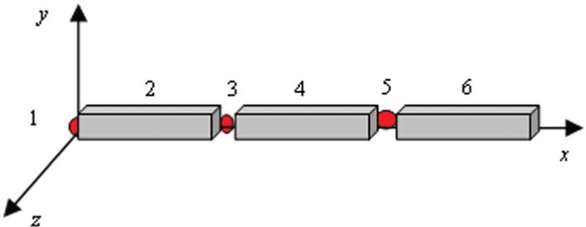
Space pendulum consisted of three rigid bodies.

The motion of the system is computed for the following initial conditions

$$\begin{array}{cc}\multicolumn{1}{c}{}& {\left[\begin{array}{c}\hfill {\theta }_x\hfill \\ \multicolumn{1}{c}{{\theta }_y}\\ \multicolumn{1}{c}{{\theta }_z}\end{array}\right]}_{2,1}={\left[\begin{array}{c}\hfill {\theta }_x\hfill \\ \multicolumn{1}{c}{{\theta }_y}\\ \multicolumn{1}{c}{{\theta }_z}\end{array}\right]}_{4,3}={\left[\begin{array}{c}\hfill {\theta }_x\hfill \\ \multicolumn{1}{c}{{\theta }_y}\\ \multicolumn{1}{c}{{\theta }_z}\end{array}\right]}_{6,5}=\left[\begin{array}{c}\hfill 0\hfill \\ \multicolumn{1}{c}{0}\\ \multicolumn{1}{c}{0}\end{array}\right]\mathrm{rad}\hfill \\ \multicolumn{1}{c}{}& {\left[\begin{array}{c}\hfill {\stackrel{·}{\theta }}_x\hfill \\ \multicolumn{1}{c}{{\stackrel{·}{\theta }}_y}\\ \multicolumn{1}{c}{{\stackrel{·}{\theta }}_z}\end{array}\right]}_{2,1}={\left[\begin{array}{c}\hfill {\stackrel{·}{\theta }}_x\hfill \\ \multicolumn{1}{c}{{\stackrel{·}{\theta }}_y}\\ \multicolumn{1}{c}{{\stackrel{·}{\theta }}_z}\end{array}\right]}_{4,3}=\left[\begin{array}{c}\hfill 0\hfill \\ \multicolumn{1}{c}{0}\\ \multicolumn{1}{c}{0}\end{array}\right]\mathrm{rad}/\mathrm{s}\hfill \\ \multicolumn{1}{c}{}& {\left[\begin{array}{c}\hfill {\stackrel{·}{\theta }}_x\hfill \\ \multicolumn{1}{c}{{\stackrel{·}{\theta }}_y}\\ \multicolumn{1}{c}{{\stackrel{·}{\theta }}_z}\end{array}\right]}_{6,5}=\left[\begin{array}{c}\hfill 0\hfill \\ \multicolumn{1}{c}{0.1}\\ \multicolumn{1}{c}{0}\end{array}\right]\mathrm{rad}/\mathrm{s}\hfill \end{array}$$

The overall transfer equation of the system is

$${\mathit{Z}}_{6,7}={\mathit{U}}_6{\mathit{U}}_5{\mathit{U}}_4{\mathit{U}}_3{\mathit{U}}_2{\mathit{z}}_{2,1}=\mathit{U}{\mathit{z}}_{2,1}$$

1. The boundary conditions are

   $$\{\begin{array}{c}\hfill {\mathit{z}}_{2,1}=[0,0,0,{\theta }_x,{\theta }_y,{\theta }_z,0,0,0,q_x,q_y,q_z,1{]}_{2,1}^T\hfill \\ \multicolumn{1}{c}{{\mathit{z}}_{6,7}=[x,y,z,{\theta }_x,{\theta }_y,{\theta }_z,0,0,0,0,0,0,1{]}_{6,7}^T}\end{array}$$

2. The dynamics of the MS are computed by MS-DT-TMM and the Newton–Euler method. ⁴⁴ The computational results of the two methods have good agreements, as shown in Figure 16, which validates the proposed method for solving multi-rigid-body system dynamics. The 1s–6s animation results of the “three-pendulum” system are shown in Figure 17.

Figure 16.

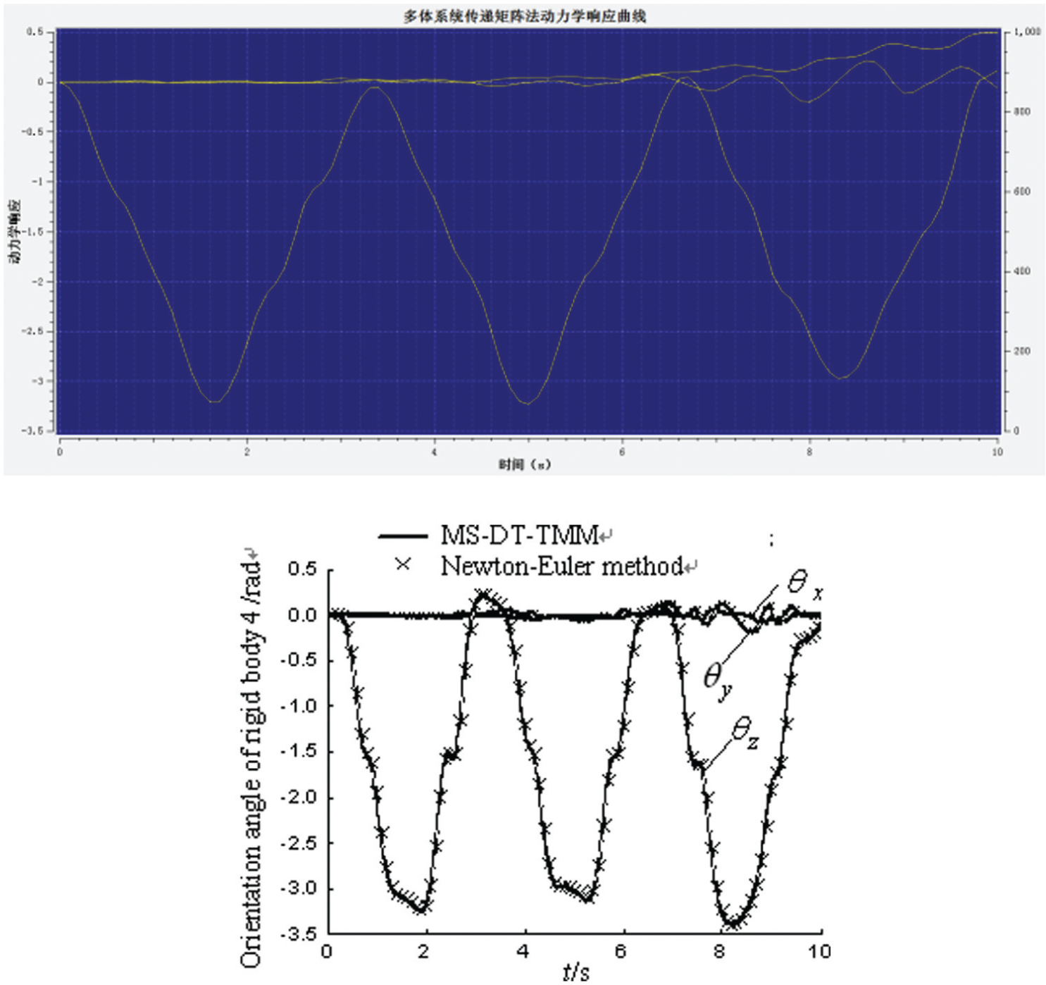
Calculation results of the azimuth of the rigid bodies 2 and 4.

Figure 17.

1s–6s animation results of a three-pendulum system.

Slider–crank example

Generally, the slider–crank mechanism is the main component of engines, compressors, punch presses, and other mechanical system. In order to verify the effectiveness of the software, the simulation of the slider–crank mechanism is given. The mechanism includes three rigid bodies (Body_Crank, Body_Conrod, and Body_Slider) and six hinges (JoClamp_Ground, JoAxrot_Ground_Crank, JoRevh_Crank_Conrod, JoInlin_Conrod_Slider, JoInlin_Ground_Slider, and JoPrism_Ground_Slider), whose connect constraint is shown in Figure 18.

Figure 18.

Structural diagram of a slider–crank mechanism.

Definition of the structural parameters of the slider–crank mechanism is shown in Table 3. The 1s–6s animation results of the slider–crank mechanism are shown in Figure 19.

Table 3.

Structural parameters of the slider–crank mechanism.

Names of parts	Parameter values
Length_Crank	0.2
Length_Conrod	0.4
Offset_Slider	0.05
Mass_Crank	1
Mass_Conrod	1
Mass_Slider	1

Figure 19.

1s–6s animation results of a slider–crank mechanism.

Engineering applications

The multiple launch rocket system (MLRS) is a type of unguided rocket artillery system. A 3D model of a type of MLRS is shown in Figure 20, which is built by UG (Unigraphics Nx, a CAD product designed by Siemens PLM Software). The users can import the STEP data into MSTMMSim.

Figure 20.

3D solid model of MLRS.

Figure 20 gives the MS dynamic model of a type of MLRS, Figure 22 shows the corresponding topology figure of the dynamic model of the MLRS. ⁵⁷ In Figures 21 and 22, the nodes of 14, 17, 20, 23, 26, and 29 are wheels; 12 is the body of truck; 10 is the revolved part; 7 is the pitch part; 3 and 1 are the launch guider; 5 is the tail of the launch guider; 6 and 8 are the joints of connection between pitch part and launch guider; 9 is the joint of connection between revolved part and pitch part; 11 is the joint of connection between revolved part and the body of the truck; 13, 16, 19, 22, 25, and 28 are the joints of connection between the wheels and the body of the truck; and 15, 18, 21, 24, 27, and 30 are the joints of connection between the ground and the wheels.

Figure 21.

Dynamic model of MLRS.

Figure 22.

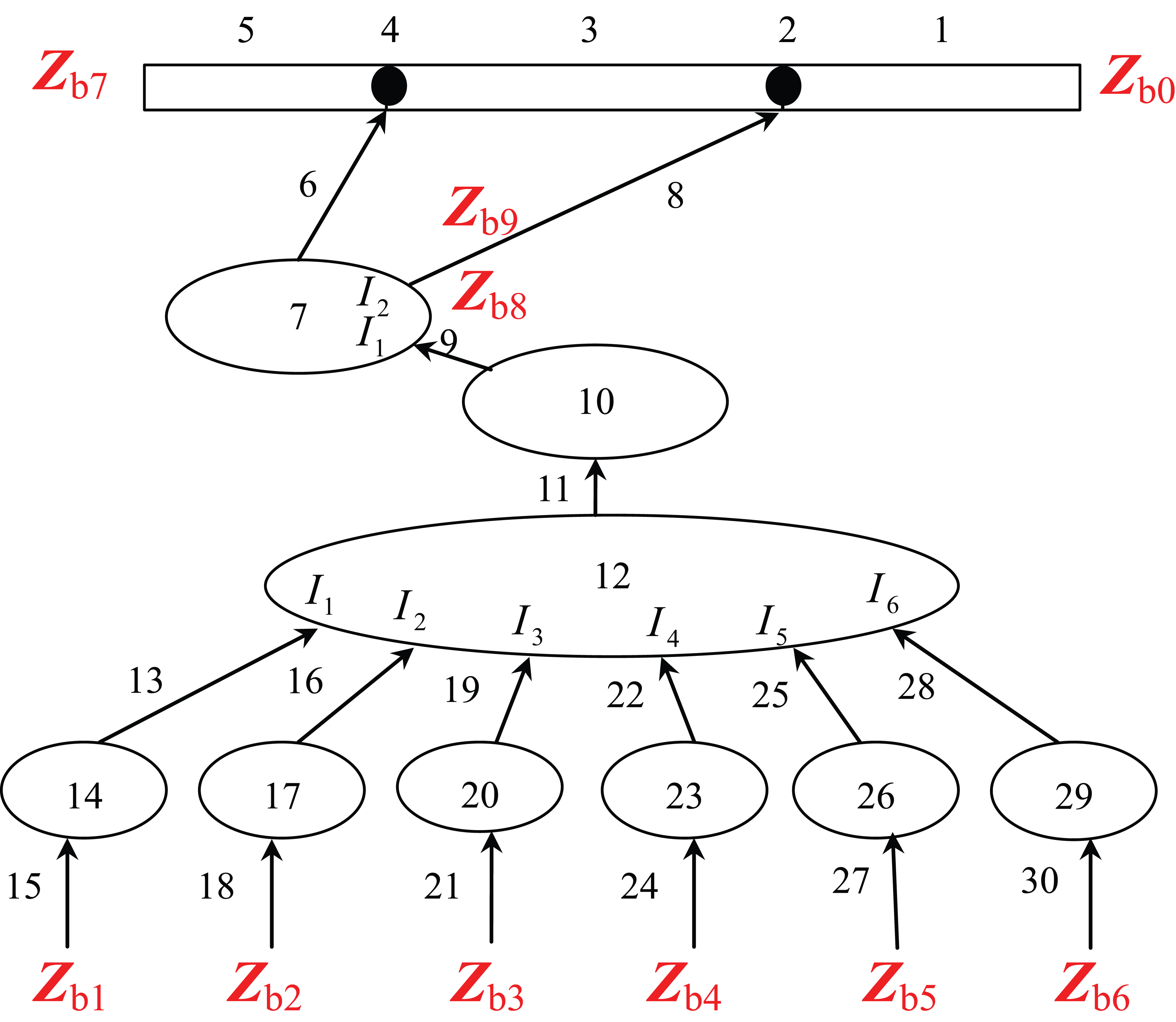
Topology figure of MLRS dynamic model.

First, the users import the STEP data generated by UG into MSTMMSim; then set the mass properties, center of mass and moment of inertia of each body, the stiffness and damping properties of each hinge, and the connection relationship of bodies through the pre-processor of MSTMMSim; and then run the MLRS MS dynamics to simulate using MSTMM solver of MSTMMSim. The animation display of the MLRS dynamic simulation and the curve of simulation results of MLRS system dynamics are performed by the post-processor of MSTMMSim as shown in Figure 23, and the simulation results of external trajectory of MLRS using Qwt 3D are given in Figure 24.

Figure 23.

Animation display of simulation of MLRS.

Figure 24.

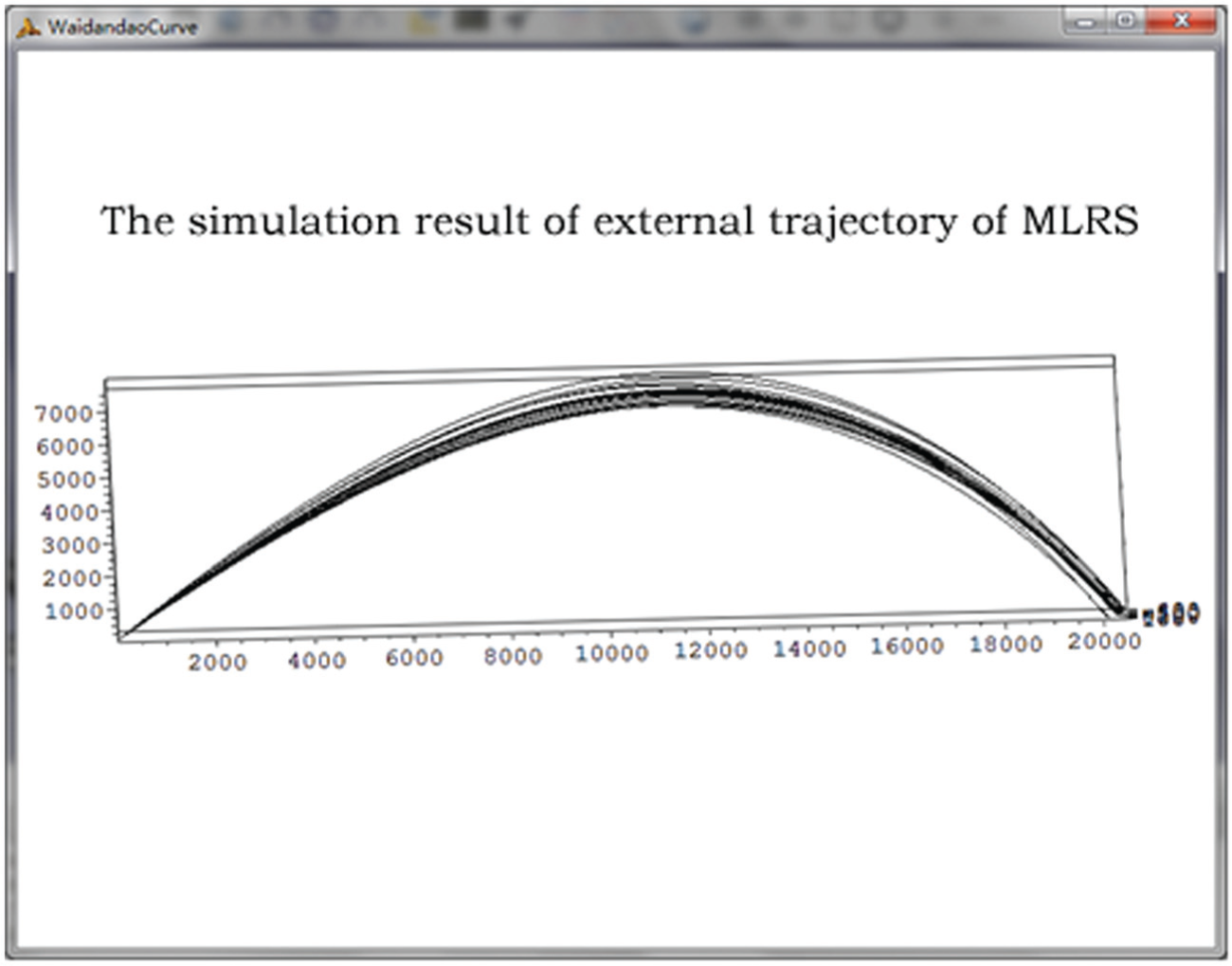
Simulation results of external trajectory of MLRS.

Operation process and computation speed of the software

Operation process of MSTMMSim

The operation process of MSTMMSim primarily includes the following steps, as shown in Figure 25:

1. Users need to build a new workspace or to open an existing workspace, as shown in Figure 25(a).

2. Users can build a mechanical system geometric model through the geometric modeling tool. If the structure of mechanical system is complex, the user can import model files from other CAD software using the import function supplied by the software, as shown in Figure 25(b).

3. Users can define the dynamic parameters of the mechanical system by the software’s GUI. The software automatically generates the dynamic parameter file of the model needed by the solver, as shown in Figure 25(c).

4. Users can choose the parameter file for the solution of the MSTMM to achieve the dynamic calculation of the mechanical system and output the calculation results, as shown in Figure 25(d).

5. Users can use animation or curve plotting module to show the calculation results, as shown in Figure 25(e).

Figure 25.

Operation process of the software.

Computation speed of MSTMM

Because MSTMM has the advantages of without the global dynamic equations of the system, low order of the system matrix, and high computational speed, use the n-rigid-pendulum system with planer motion as an example to compare the time cost using MSTMM with that using Newton–Euler method. And the CPU of the used microcomputer is an Intel Core i7 2.6 GHz. It can be seen clearly from Figure 26 that the computational time increases very slowly when the number of the degrees of freedom increases when using MSTMM, and the computational time increases very quickly when the number of the degrees of freedom increases when using ordinary methods; the time consumption of MSTMM is much less than that of Newton–Euler method, when the MSTMM has a higher computational speed. Of course, now, the building of the global dynamic equations of MSs can also be relatively simple using some effective methods, and using the sparse matrix techniques, the computer time is directly proportional to the number of the bodies for chain system, so that computational speed can also be increased greatly.

Figure 26.

Cost time compare with MSTMM and Newton–Euler Method.

Conclusion

This article takes the advantages of fast computing, flexible modeling, and high degree of programming of the MSTMM to develop generic virtual design software for mechanical system dynamics. The examples show that the MSTMMSim has the following features:

1. Fast calculation speed, user-friendly interface, using an MDI QT framework to achieve a multi-window interaction design.

2. Application of OCC geometry generation function in a multibody dynamic simulation software can import a variety of CAD files; MS dynamic software directly calls CAD results.

3. The software realizes the rapid calculation for the MS dynamics based on the MSTMM.

4. Suitable for various topologies of MS dynamics. The software uses a multi-tier architecture which is of low coupling and strong expansion, providing a powerful, dynamic design tool for weapons, ships, aeronautics, astronautics, vehicles, and general machinery industries.

In the future, we will strengthen the software through the following aspects: first, further improve the MSTMM solver and add parallel computing capabilities to improve computing speed; and second, add a variety of expansion modules, such as vibration analysis module, linear analysis module, experimental design, and analysis module.