
Abstract
The transfer matrix method for multibody system is a new method developed in recent 20 years for studying multibody system dynamics. The new version of transfer matrix method for multibody system and automatic deduction theorem of system overall transfer equation have been formed in 2012. The overall transfer equation plays one of the key roles for transfer matrix method for multibody system. In order to study branch system dynamics with new version of transfer matrix method for multibody system, the automatic deduction theorem of overall transfer equation has been expanded in this article, which made it practicable to deduce automatically the overall transfer equation for branch system with new version of transfer matrix method for multibody system. The transfer equations and transfer matrices of typical elements are developed for the automatic deduction theorem of overall transfer equation. Thereby new version of transfer matrix method for multibody system owns the following features: there is no need to establish the global dynamics equation of system, by which the study on multibody system dynamics will be simplified greatly; the automatic deduction of overall transfer equation for multibody system is realized, consequently the algorithm is simple and highly programmable; moreover, the order of system matrix is always low, which result in high computational speed. The branch multibody system dynamics has been computed with the automatic deduction theorem of overall transfer equation as well as ordinary multibody system dynamics method. The computational results obtained by the two methods have good agreements, which validate the automatic deduction theorem of overall transfer equation for branch multibody system.
Keywords
Introduction
The dynamics equation of an individual rigid body that established by Newton’s 1 Law and Euler 2 Theorem has promoted the development of rigid body dynamics and mechanical system dynamic design technology. Under strong engineering demand, a new subject branch, multibody system dynamics,3–9 has been developed step by step since 1960s. The deduction of system dynamics equation and its numerical solution are the two most important parts for studying multibody system dynamics (MSD). Increasing computational speed and accuracy is one of the important research areas for complex multibody system dynamics. The recursive Newton Euler algorithm was presented 10 to increase the computational speed.
The classic transfer matrix method (TMM) has been developed in 1920s for studying vibration problems of one-dimensional system constructed by elastic components. 11 Holzer 25 (1921) was the very first to solve torsional vibration problem of multi-disk shaft with initial parameter method. Myklestad 26 (1944) solved beam bending vibration model with the method similar to Holzer’s. Proh 27 (1945) successfully generalized Holzer’s method to transverse vibration problem of shaft. Due to the development of computer and application of matrix operation in vibration research, Myklestad’s method has been progressively developed to TMM. Thomson 28 (1950) applied TMM on structure vibration problem of general linear system. Pestel and Leckie 12 published the first book of TMM “Matrix Method in Elastomechanics.” Rubin 29 (1964) proposed the general treatment process of transfer matrix as well as the relationship between transfer matrix and frequency response matrix with other form. With TMM, Targoff, Lin, Mercer, Lin, Mead, Henderson, McDaniel, and Murthy, respectively, solved statics and dynamics problems of beam, beam-type multiple structure, board with string, ribbed structure, curved multi-span structure, cylindrical shell, rigid ring, and so on. Horner 30 (1978) proposed the numerical stability of Riccati TMM while solving boundary value problem. Combined with TMM and finite element method (FEM), Dokanish 31 (1972) proposed the FE-TMM to solve two-dimensional thin board and increased the computational speed of FEM. 13 Combined with TMM and numerical integrating method, Kumar and Sankar 14 developed the discrete-time transfer matrix method (DTTMM) for time-variant system structure dynamics.
In order to meet the requirement for increasing the computational speed of MSD and simplifying the research process of MSD, Rui with his cooperator proposed the transfer matrix method for multibody system (MSTMM):11,14–24 in 1993, for the first time, the linear MSTMM has been proposed, the huge computation workload of eigenvalue problem of complex linear multibody system as well as the ill condition brought by large stiffness gradient has been solved while the computation efficiency has been increased; in 1997, the new concept of linear multibody system augmented eigenvector and augmented operator have been proposed, multi-rigid-flexible-body system augmented eigenvector with orthogonality has been constructed, the accurate analysis of the dynamics response of complex multi-rigid-flexible-body system has been realized with modal method;11,15,16 in 1998, the DTTMM for multi-rigid-body system15,17 has been proposed and improved progressively; through time-variant transfer matrix and state vector with state variable described by physical coordinates, the computational speed of multibody system dynamics has been greatly increased; in 1999, the DTTMM for multi-rigid-flexible-body system has been15,18 proposed and the high-speed computation of multi-rigid-flexible-body system dynamics has been realized; in 2005, the TMM for two-dimensional system has been proposed, and two-dimensional system dynamics analysis with pure TMM has been realized; 19 the mixed method with MSTMM and ordinary multibody system dynamics (MSDM), mixed method with MSTMM and FEM, linear controlled MSTMM, controlled discrete-time transfer matrix method for multibody system (MSDTTMM),20,21 Riccati MSDTTMM, 22 and finite section MSDTTMM have been proposed, respectively; the overall transfer equation is one of the key roles for MSTMM; and in 2012, the automatic deduction theorem 23 of overall transfer equation has been proposed and the automatic deduction of overall transfer equation has been realized; the new version of MSTMM 24 has been proposed, thereby the research of MSD and the application of new version of MSTMM for numerous engineering technicians have been simplified.
The original automatic deduction theorem of overall transfer equation 23 is effective for general system for linear MSTMM and MSDTTMM, also effective for the chain system and closed-loop system for the new version of MSTMM. In this article, the automatic deduction theorem of overall transfer equation for branch system for new version of MSTMM has been established. The original automatic deduction theorem of overall transfer equation has been expanded and the corresponding transfer equations and transfer matrices of typical elements have been deduced. The automatic deduction of overall transfer equation for branch multibody system has been realized, also with the result of simple algorithm and high programming. The MSD has been computed using the automatic deduction theorem of overall transfer equation for branch system and ordinary MSDM, respectively, with the good agreements of both results, the effectiveness of automatic deduction theorem of overall transfer equation for branch multibody system has been validated.
Principles and steps of new version of MSTMM
Multibody system dynamics model topology graph and label convention
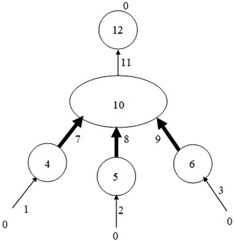
The topology graph of MSD model is a new graph notation for new version of MSTMM that describes the transfer relationship, position sequence numbers, boundary sequence numbers, and transfer direction among the state vectors of body elements and hinge elements 23 in MSD. The branch MSD model topology graph shown in Figure 1 is taken as an example for detailed description.

Topology graph of dynamics model of a branch system.
According to the features of new version of MSTMM, the label conventions in this article are as follows:
Mechanics elements are divided into two types—“bodies” and “hinges”—and are numbered uniformly. A body with only two joints connecting with other elements, including boundary, is treated as the element with single-input end and single-output end. A body with more than two joints connecting with other elements is treated as the element with multi-input ends and single-output end. The element j in the transfer path from tip element n to element i and connects directly with element i is named as the inboard element (inboard body or inboard hinge) of element i, the element i is named as the outboard element (outboard hinge or outboard body) of element j.
In topology graph, a circle ○ and the number inside it indicate, respectively, a body element and its sequence number; an arrow → and the number beside it indicate, respectively, a hinge element and its sequence number, the arrow direction shows the transfer direction of state vector, and number 0 in the figure means the system boundary.
For a non-boundary end, the bold italic small letter

is the column matrix in global inertial coordinates system oxyz. And
4. Only one of the boundary ends in a system is called the root, whose state vector is
5. The transfer directions of system state vectors are always from tips to root. Along transfer direction, the nodes entering an element are called input ends of the element, at the meantime are denoted as I, while the node leaving an element is called the output end of the element and is denoted as O. The connection point between elements is the output end of its inboard element and at the same time is the input end of its outboard element.
6. Conventions of positive direction for torques and forces: Inboard forces and outboard torques acting on an elements are positive (negative) if their vectors are in positive (negative) directions, outboard forces and inboard torques acting on an elements are positive (negative) if their vectors are in the negative (positive) direction.
7. The boldface italic capital
The motion of every element in the system is described in right-handed inertial Cartesian coordinate system oxyz; x, y, and z are used as the position coordinates of element joint. The origin point of body-fixed coordinate system

Inertial Cartesian coordinate system oxyz and body-fixed coordinate system
Principle of new version of MSTMM
The basic idea of MSTMM is: break up a complicated multibody system into many elements including bodies and hinges whose dynamics properties can be readily expressed in terms of matrices. These transfer matrices of elements are like construct bricks while the library of transfer matrices can be readily developed. When assembled them together according to topology structure of the system, the dynamics properties of entire system can be provided. For chain system, the overall transfer matrix and overall transfer equation of system can be obtained by simply successive multiplying of transfer matrices of elements. According to Newton’s third law, for any two adjacent elements in multibody system, the state vectors of the output end of inboard element and of the input end of outboard element are always equivalent.
It can be proved that there is the direction cosine matrix 6 from body-fixed coordinate system to inertial coordinate system

The angular velocity

where


It should be pointed out that any kind of Euler angle formulation has its inherent singularity, that is why the angular acceleration
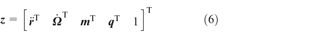
The state vector, transfer equation, and transfer matrix of element
For convenient description, herein a chain system is taken as an example. The state vector of spatial motion element in joint is defined as equation (1) or
where

Particularly, for the chain system with planar motion

Applying above definition of state vector, according to Newton’s second law and Euler theorem, there is linear relationship among the acceleration and angular acceleration of any object and the external force and external torque acting on it in inertial coordinate system, which can be expressed as linear algebraic equation in matrix form, that is, for any element j with two ends, if its definition of the state vector is expressed as equation (1), the following equation has always been strictly satisfied

Equation (9) described the transfer relation between state vectors in two ends of element j, thus is named as the transfer equation of element j;
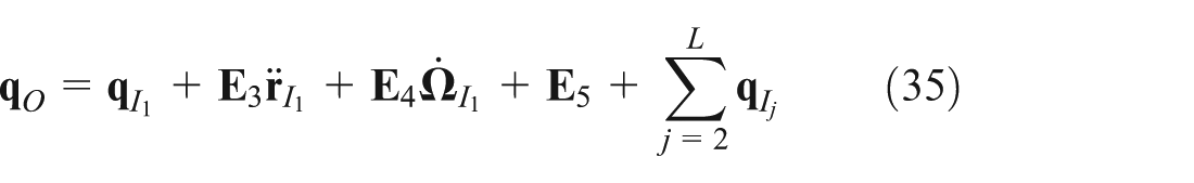
System overall transfer equation and overall transfer matrix
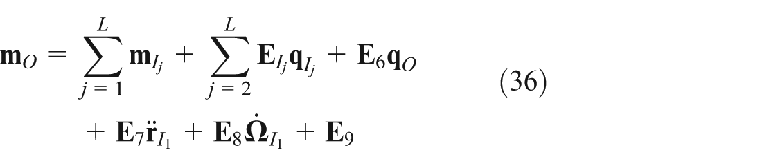
For chain system constructed by n elements, applying repeatedly the element transfer equation (equation (9)), the system overall transfer equation that connects two ends of the system can be obtained

where

is the overall transfer matrix of system.
It can be seen from equations (10) and (11) that the overall transfer matrix
Solution of system dynamics
Applying boundary condition and initial condition of the system, such as the initial position coordinate, absolute velocity, rotation angle, and angular velocity, solving overall transfer equation of the system equation (10) and transfer equation of element equation (9) one after another, the state vector of each element at
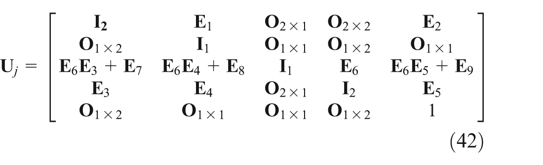
Transfer equations of typical elements
Transfer equation of spatial motion rigid body with single-input end and single-output end
For spatial motion rigid body j with single-input end and single-output end, as shown in Figure 2, the position vector of rigid body input end I and any point P in the body is
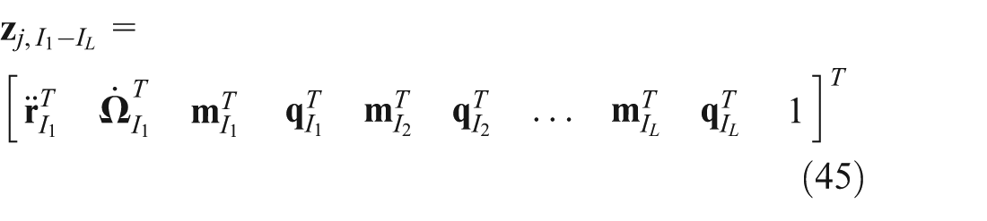
The position vector of any point P in rigid body

taking the derivative and the second derivative with respect to time, one obtains


The angular velocity and angular acceleration of any point P and input end I are respectively equal for rigid body, that is


Considering label convention, the rigid body dynamics equation in oxyz can be expressed as


Rewrite equation (14) and dynamics equations of rigid body equations (17) and (18)


Note the state vector definition equation (6), the transfer equation, and transfer matrix of spatial motion rigid body j with single-input end and single-output end can be obtained by rewriting system dynamics equation


where
Transfer matrix of spatial large motion rigid body with multiple inputs and single output
For rigid body j with multi-input ends and single-output end as shown in Figure 3, one end is regarded as output end, all other ends are regarded as input ends;

Spatial motion rigid body with multi-input ends and single-output end.
Note the derivative and the second derivative of


and

According to rigid body kinematics, the relationship between acceleration of the first input end and output end of rigid body


The geometric equation of the first inboard end


Considering label convention, the rigid body dynamics equation in oxyz can be expressed as


Rewrite equation (29) and dynamics equations of rigid body equations (32) and (33)

where

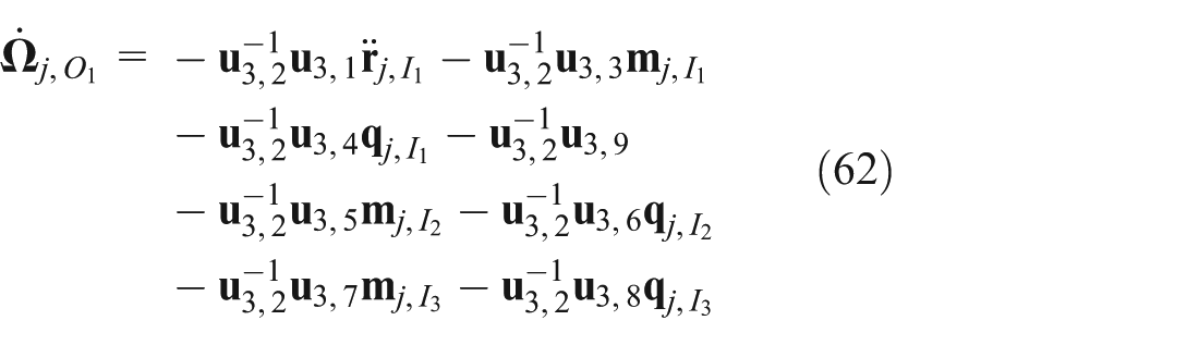
The state vector of rigid body outboard end is defined as equation (6), and the comprehensive state vector of input ends is defined as

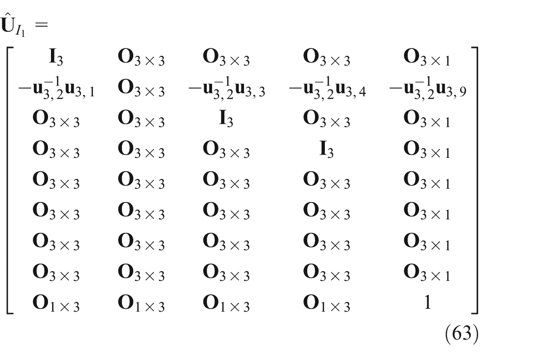
where the first subscript j of comprehensive state vector of the input end denotes the sequence number of outboard body of multiple hinges subsystem, the second subscript
According to the acceleration and internal force equations (35) and (36) and the definition equations (6) and (38) of state vector of output end and comprehensive state vector of input ends of rigid body, the transfer equation and the transfer matrix of spatial motion rigid body with multi-input ends and single-output end can be obtained


Transfer equation of rigid body with planar large motion
Notice the definition equations (8)–(10) of the state vector of planar motion multibody system, similarly, the transfer equation and transfer matrix of planar motion rigid body j with single-input end and single-output end can be obtained

where

And, the transfer matrix of planar motion rigid body with multiple input ends and single-output end can be obtained

where


Transfer equation of smooth ball-and-socket hinge with spatial large motion
For smooth ball-and-socket hinge j with spatial motion inboard body


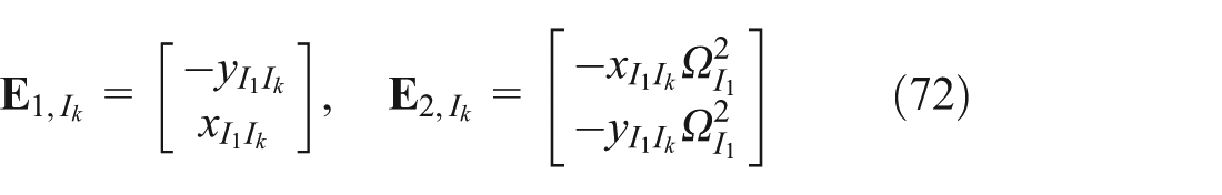
where
For the smooth ball-and-socket hinge whose outboard hinge is fictitious hinge (end free), the internal torque at two ends of its outboard body are both zero, thus the transfer equation and transfer matrix of such smooth ball-and-socket hinge are the same as equations (48) and (49).
Transfer equation of smooth pin with planar large motion
For smooth pin j with planar motion inboard body

and the transfer matrix is

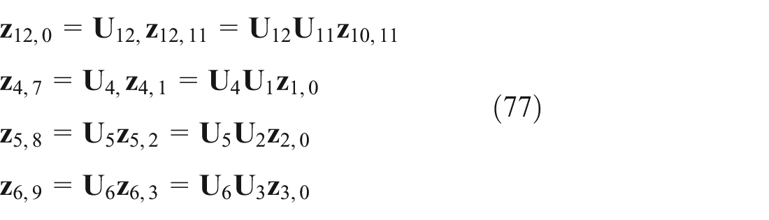
where
For the smooth pin whose outboard hinge is fictitious hinge (end free), the transfer equation and transfer matrix of such smooth pin are the same as equations (50) and (51).
Automatic deduction method of overall transfer equation for branch multibody system
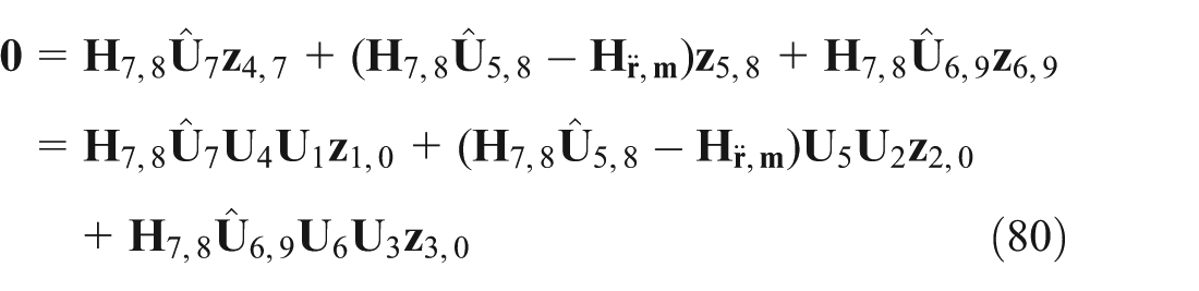
In Rui et al., 23 the automatic deduction theorem of overall transfer equation has been proposed, which is effective to any system for linear MSTMM and MSDTTMM, and is also effective to chain system and closed-loop system for new version of MSTMM. It is because that the smooth hinge can be treated as special elastic hinge with very small torsional stiffness for any topology structure, the transfer matrices of all elements along transfer path and direction exit. For new version of MSTMM, chain system and closed-loop system, the transfer matrices of all elements exit along the transfer path and transfer direction. The automatic deduction theorem of overall transfer equation for new version of MSTMM has been developed in this article so that effective to branch system.
Main transfer equation of multi-hinge subsystem with spatial motion
For the subsystem of multiple smooth ball-and-socket hinges with spatial motion or pin hinges with planar motion in the branch system as shown in Figure 1, due to the outboard body is the same rigid body with spatial motion as shown in Figure 4 in terms of thick arrow, it is treated as subsystem with multiple input ends and multiple output ends. Its transfer equation includes two parts which are the main transfer equation and geometric equations. The main transfer equation describes the relation among the acceleration, angular acceleration, internal torque, and internal force acting on element. While geometric equations describe the relation among the acceleration and angular acceleration between the first input end and the kth
Subsystem of multiple smooth ball-and-socket hinges with the same outboard body.
The definition of state vector of each input end in multi-hinge subsystem is

The definition of the comprehensive state vector of all output ends in multi-hinge subsystem is the same as the comprehensive state vector of input ends of the rigid body with multi-input ends as follows

where the first subscript i and j of state vector denote, respectively, the sequence numbers of inboard body and outboard body of the hinge, while the second subscript
It can be proved that the main transfer equation describes the relationship among the comprehensive state vector of output ends and state vectors of each input end in the multi-hinge subsystem is

where the coefficient matrix
Then, we deduce the coefficient matrix of state vector in the main transfer equation (54). In the multi-hinge subsystem with multi-input ends and multi-output ends with the same outboard body, accelerations, internal torques, and internal forces are equivalent at input and output ends for each hinge


If the output end of outboard body of the hinge is also connected with a smooth hinge, according to the transfer matrix of the outboard body, we have

therefore

after transposing, one obtains
expressing as the form of equation (54), one obtains
For multi-hinge subsystem with planar motion, the column quantities of null matrix and identity matrix in coefficient matrices


For the branch system shown as Figure 4, the coefficient matrix of state vector
Geometric equation of spatial motion multi-hinge subsystem
The output ends of the multi-hinge subsystem are corresponding to the input ends of the outboard body. The relationship among the acceleration of the first input end and other input ends of the outboard rigid body satisfies acceleration composition theorem. The accelerations of input end and output end of individual smooth hinge are equivalent, so the relationship among acceleration of hinge corresponding to the first input end of outboard rigid body and the accelerations of input ends of other hinges satisfy acceleration composition theorem. The relationship among acceleration of hinge corresponding to the first input end of outboard rigid body and the accelerations of input ends of other hinges, is expressed by comprehensive state vector and state vectors of input ends of other hinges corresponding to non-first input end, complemented with the parts that torques are zero at input and output ends of smooth hinge, and is named as the geometric equation of multi-hinge subsystem

where
Then solve extraction matrix
Each input end and the first output end in multi-hinge subsystem satisfy the following relationship


where

Rewriting as the form of equation (65), one obtains


Transfer equation of planar motion multiple smooth pins subsystem with the same outboard body
Note that for planar motion multiple smooth pins subsystem with the same outboard body

Equation (68) becomes
Then main transfer equation and its coefficient matrix of state vector, geometric equation, acceleration and internal torque extraction matrix, associated matrix of the comprehensive state vector corresponding to
Overall transfer matrix of branch multibody system
As shown in Figure 4, for the branch system where smooth hinges 7, 8, and 9 connect with the same outboard rigid body 10, the outboard body 10 is regarded as body with multi-input and single-output end, the transfer equation between comprehensive state vector of input ends and state vector of output end have been developed. Smooth hinges 7, 8, and 9 are regarded as a multi-input and multi-output subsystem, develop the main transfer equation and geometric equation among state vector of each input end and comprehensive state vector of output end; then the overall transfer matrix of branch system can be obtained.
For multi-hinge subsystem, the state vectors of each input end

and geometric equations

where

is the comprehensive state vector of output end of multi-hinge subsystem. The state vectors of all input ends of rigid body with multi-input ends and single-output end are uniformly expressed by a comprehensive state vector
One can deduce the main transfer equation of rigid body 3 with multi-input ends and single-output end

where
It is easy to obtain the transfer equations of other elements in Figure 4
According to system dynamics model topology and the transfer equations of elements and subsystem equations (73), (76), and (77), the system main transfer equation is obtained

where

Express the state vector in geometric equation (equation (74)) with the state vector of system boundary ends

or write as


where
The system overall transfer equation is composed by system main transfer equation (78) and the geometric equations (equations (82) and (83)) of all multi-hinge subsystems with the same outboard body

or write as

where


Rewrite equations (87) and (88) as the following form


where


Define the state vector
Automatic deduction theorem of overall transfer equation of branch multibody system
From equation (86), the following characteristics of overall transfer equation for new version of MSTMM can be obtained, which form the automatic deduction theorem of overall transfer equation for branch multibody system:
The state vector involved in the overall transfer equation is system boundary state vector
The overall transfer equation is composed of main transfer equation and geometric equations. In the main transfer equation, the coefficient matrix of the system boundary state vector corresponds to the first row of the overall transfer matrix; the coefficient matrix of root state vector is minus identity matrix. The structure of the coefficient matrix
The structure of coefficient matrix of tip state vector in geometric equations of branch system such as equations (85) and (86) obeys the following rules: the coefficient matrix from tip to the first input end of body with multi-input ends (such as
3. For chain system and closed-loop system, automatic deduction theorem of overall transfer equation and the form of overall transfer matrix are the same for new version of MSTMM and for MSTMM.
Above-mentioned automatic deduction theorem is effective for various multi-rigid-body system, chain multi-rigid-flexible-body system, closed-loop multi-rigid-flexible-body system, and tree multi-rigid-flexible-body system that the multi-end bodies in the system are rigid bodies.
Algorithms for dynamics analysis
The algorithm using the proposed method for dynamics analysis is shown as follows:
Decide the initial condition, system parameters and boundary conditions of the multibody system.
Set
Knowing the initial conditions such as position coordinates, velocities, rotation angles, and angular velocities
Apply system boundary conditions and overall transfer equation, compute unknown state variables in every boundary state vector
After the entire state vectors in boundary have been solved, state vector of each element can be obtained by solving the element transfer equation successively.
Apply initial conditions
Let
Repeat above steps, until the time required for complete analysis.
Numerical examples
As shown in Figure 4, body 12 of the branch system is hang on ceiling by smooth ball-and-socket hinge, in other words, the boundary of body 12 is simply support. Boundaries of body 4, 5, and 6 are free. That is


There are system initial conditions: the initial rotation angles and angular velocities of rigid body 12, 10, 4, 5, 6


solve the system motion under gravity.
Set axis y is opposite with the gravity direction. In the figure, hinge 11, 7, 8, and 9 are all smooth ball-and-socket hinges; body 12, 4, 5, and 6 are rigid bodies with single-input end and single-output end and the same structure parameters, rigid body mass
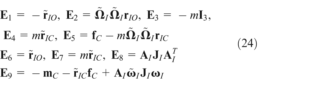
The overall transfer equation, state vector, and overall transfer matrices of the system are shown as equations (86)–(88), respectively. The transfer equations and transfer matrices of rigid body with single-input end and single-output end, of smooth hinge with single-input end and single-output end, of rigid body with three input ends and single-output end, and of three-smooth ball-and-socket hinges subsystem are shown as equations (22), (23), (45), (46), (50), (51), (54), (63), and (64), respectively. The computational results of time history of rotation angles of the five rigid bodies that obtained by new version of MSTMM with automatic deduction theorem of overall transfer equation and automatic dynamic analysis of mechanical systems (ADAMS) are shown in Figure 5. The results obtained by the two methods have good agreements, which validate the automatic deduction theorem of overall transfer equation for branch multibody system.

Rotation angle of each rigid body obtained by new version of MSTMM and ADAMS.
The computational speed is very important for multibody system with large degrees of freedom (DOF). Herein, a new system with a chain subsystem composed by the same 245 rigid bodies and hinge as body 4, 5, 6, and 12 in the above numeric example is connected with body 12. The initial rotation angles and angular velocities of all the new rigid bodies are the same

The DOF of the system is 750. The dynamics of the system is computed respectively with both the proposed method and ADAMS.
The computational results of time history of rotation angles of the four boundary rigid bodies as well as the body with multi-input ends obtained by new version of MSTMM with automatic deduction theorem of overall transfer equation and by ADAMS are shown in Figure 6, while the computational time is shown in Table 1.

Rotation angles of tip and root rigid body obtained by new version of MSTMM and ADAMS.
Computational time comparison.
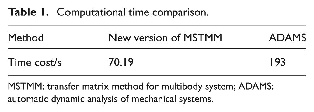
MSTMM: transfer matrix method for multibody system; ADAMS: automatic dynamic analysis of mechanical systems.
The time measurement of the proposed method and ADAMS are made with the same CPU environment on Windows. Both the results are picked as average of 10 times of computations, in order to reduce the effect of background tasks. The settings of the solver are shown in Figure 7.

Solver settings.
The results obtained by the two methods have good agreements, which validate the automatic deduction theorem of overall transfer equation for branch multibody system. The computational speed of new version of MSTMM is much higher than ADAMS.
Conclusion
On the research work basis of new version of MSTMM, 24 the principle equation of new version of MSTMM has been elaborated and expanded in this article. According to the foundational principle, transfer equation and transfer matrix of element, overall transfer equation, and overall transfer matrix of system, in new version of MSTMM, are accurate and boundary conditions satisfied; it has been elaborated that new version of MSTMM, in principle, belongs to accurate analysis method of MSD. Proceed from the deduction of the basic transfer equations and transfer matrices of rigid body with multiple input ends, multi-hinge subsystem with multiple input ends and multiple output ends, the concept of topology graph of system dynamics model has been expanded, the automatic deduction theorem of overall transfer equation for branch system has been formed for new version of MSTMM, by which the sphere of application of the automatic deduction theorem 23 of overall transfer equation for branch multibody system has been expanded from linear MSTMM, MSDTTMM to new version of MSTMM.
The computational results of the multibody system dynamics obtained by both automatic deduction theorem of overall transfer equation for branch system and ordinary multibody system dynamics method have good agreements, which validate the automatic deduction theorem of overall transfer equation for new version of MSTMM.
Footnotes
Acknowledgements
The first author of this paper owns special thanks to Prof. Dieter Bestle from Branderburgische Technische Universität for his constructive suggestions and modifications for this paper. Also special thanks to Prof. Peter Eberhard and Prof. Werner Schiehlen for their offer of very kind help and great guidance during the first author’s study in Stuttgart University. The authors own special thanks to Dr Wenbing Tang, Dr Qinbo Zhou, Dr Junjie Gu, Dr Haigen Yang, Dr Yan Wang, and Dr Dongyang Chen for their help.
Academic Editor: Fen Wu
Declaration of conflicting interests
The author(s) declared no potential conflicts of interest with respect to the research, authorship, and/or publication of this article.
Funding
The author(s) disclosed receipt of the following financial support for the research, authorship, and/or publication of this article: Research in this paper was supported by Research Fund for the Doctoral Program of Higher Education of China (20113219110025 and 20133219110037), Nature Science Foundation of China Government (11472135), and Program for New Century Excellent Talents (NCET-10-0075).