A simple control algorithm for controlling biped dynamic walking with stopping ability based on the footed inverted pendulum model

Abstract

In biped walking, dynamic balance ability is an important evaluation index. Zero-moment-point-based trajectory control is a common method for biped dynamic walking, but it requires complex control mechanisms that limit its applications. With the help of passive dynamics, the biped walking based on the inverted pendulum model can achieve dynamic walking in a simple way; however, it has no stopping ability, which is necessary for practical use. To solve this problem, this article proposes a footed inverted pendulum model and develops a simple three-part decomposition control algorithm for controlling biped dynamic walking based on the model. In the control algorithm, the biped walking is decomposed into three separate control parts: body posture, body height, and body velocity. Body posture is controlled by the stance hip, body height is controlled by the stance knee, and body velocity is controlled by the stance ankle and swing foot placement simultaneously. A simulation is presented to analyze the foot’s effect on the inverted pendulum model. Two hardware experiments exploring velocity control and balance are described, with the results showing that the biped can achieve dynamic walking with stopping ability by using the simple control algorithm based on the footed inverted pendulum model.

Introduction

Robots that move on two legs are called biped robots. Biped robots fall down easily compared to the wheeled robots, four- or more- legged robots, such that the dynamic balance ability is an important evaluation index for biped walking. A common method for biped dynamic walking is zero moment point (ZMP)-based trajectory control.^1–4 According to the published paper, humanoid robots such as those created by the Humanoid Robotics Project, ⁵ Honda, ⁶ and the Korea Advanced Institute of Science and Technology ⁷ utilize ZMP-based trajectory control. However, this method specifies a nominal trajectory about which the system is tightly controlled.^8,9 This condition restricts widespread applications of the biped robots and creates a demand for a simpler control algorithm for biped walking.

One extreme simple control method for biped walking is no active control, this motion pattern, proposed by McGeer,^10,11 is called “passive dynamic walking.” Garcia et al. ¹² used an inverted double pendulum model with one body mass and two leg masses to illustrate passive dynamic walking; one inverted pendulum makes contact with the ground as the stance leg, while the other acts as the swing leg. The stance leg and the swing leg move by the action of gravity and inertia. McGeer ¹⁰ and Collins et al. ¹³ built two-dimensional and three-dimensional passive dynamic walking robots, respectively. These biped robots can walk down a ramp independently, relying only on gravity and inertia. The motion character of the passive dynamic walking robots is its fixed walking parameters determined by mechanical structure, for example, the step period is determined by leg length, ramp slope, and body and leg masses. Passive dynamic walking demonstrates that biped walking can be controlled through simple means. However, passive dynamic walking robots are most commonly used as children’s toys, ¹⁴ and they are not applicable in practical settings because they cannot sustain steady walking on level ground. Furthermore, they are highly sensitive to disturbance, ¹⁵ these problems raise the question of how to regulate the motion of a passive dynamic walking robot for practical applications.

If active controls are added to a passive dynamic walking robot, its motion pattern is no longer a purely passive dynamic process, although its walking performance improves. Actively controlling the swing foot placement and the stance leg length are two ways to regulate biped motions in practice.^16–18 Actively controlling the swing foot placement means that the swing leg’s motion is no longer a passive dynamic process, and actively controlling the stance leg’s length has the same consequences for the stance leg’s radial motion. With these adjustments, only the stance leg’s rotating motion remains a passive dynamic process. Based on this method, the walking robot Ranger created by Bhounsule et al. ¹⁵ achieves stable walking with dynamic balance in a relatively simple way. The motion character of walking robot Ranger is its velocity stabilize ability. It increases step length to decelerate when walking faster and increases the stance leg push-off to accelerate when walking slower. However, although the biped based on inverted pendulum model (IPM) can achieve dynamic walking, it is statically unstable; it tends to fall down when standing still. ¹⁴ Bionics research demonstrates that human walking is not only balanced by the swing foot touchdown but also balanced by the stance ankle torque. ¹⁹ The foot is ignored in the IPM, with the result that the biped cannot stand still and has no stopping ability. If a biped can walk but not stop, or can only stop walking by falling down, it cannot be used in practical applications.

In order to realize the biped dynamic walking with stopping ability in a simple way, this study connected a foot to the end of an inverted pendulum to create the footed inverted pendulum model (FIPM). The connection point between the stance foot and the end of the inverted pendulum is called stance ankle. To avoid tight position controlling of the rotation motion of the FIPM, in this article, the stance ankle is controlled by torque so that the rotating motion of the FIPM will have the compliant character to disturbances. The structure of this article is as follows: the definition and dynamic analysis of the FIPM are detailed in section “The dynamic equations for FIPM,” the establishment of decomposition control algorithm with dynamic balance based on the FIPM is given in section “Control algorithm,” the comparison of the biped motion state different change between the IPM and the FIPM is explained in section “Comparative analysis in phase-plane,” the analyses of the kinematics relation between the FIPM and biped robot is shown in section “Joints control of the biped robot,” and the experiment carried out and verification of the effectiveness of the control algorithm is shown in section “Experiment and results” last.

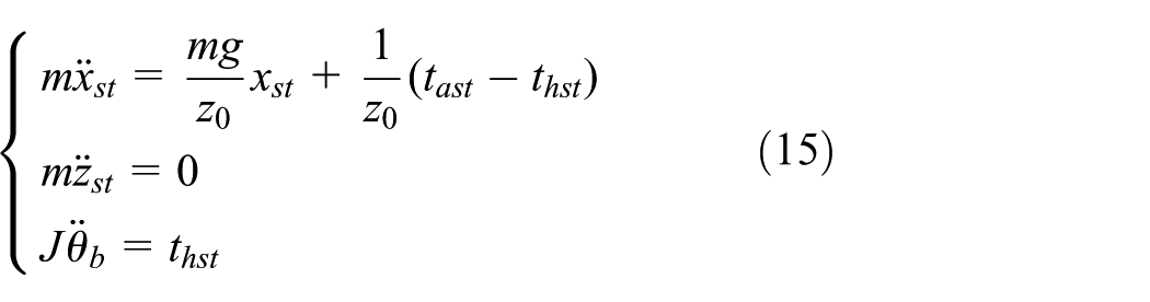
The dynamic equations for FIPM

Figure 1 shows the FIPM proposed in this article. This model is composed of three parts: a body with mass m and rotational inertia J, a massless telescopic leg, and a massless foot. The leg is connected to foot by rotational joint with torque $t_{\mathrm{ast}}$ at leg angle ${\theta }_{\mathrm{lst}}$ , the body is connected to the stance leg by the rotational hip joint with torque $t_{\mathrm{hst}}$ at body pitch angle ${\theta }_b$ , and the foot height is H.

Figure 1.

The footed inverted pendulum model: (a) overall structure, (b) the force analysis of inverted pendulum part, and (c) the force analysis of foot part.

The defining characteristic of this model is the foot, which can provide a finite ankle torque $t_{\mathrm{ast}}$ . The value range of ankle torque is determined by the ZMP value range of stance foot in order to guarantee the foot pad makes contact with the ground. With the active adjustment of the stance ankle torque $t_{\mathrm{ast}}$ , the rotational motion of the FIPM is no longer a completely passive motion. When the biped is in a critical state, any tendency toward falling down can be corrected instantaneously, so that the biped can obtain a stopping ability.

In this article, the dynamic equation of the FIPM is deduced by the Lagrangian method according to Figure 1(a) and (b).

The kinetic energy T of the FIPM is represented as follows

$$T=\frac{1}{2}m{\stackrel{.}{x}}_{st}^2+\frac{1}{2}m{\stackrel{.}{z}}_{st}^2+\frac{1}{2}J{\stackrel{.}{\theta }}_b^2$$

(1)

The potential energy U of the FIPM is composed of four parts: gravitational potential energy $U_1$ of the body, contractility potential energy $U_2$ of the leg, torque potential energy $U_3$ of the ankle joint, and torque potential energy $U_4$ of the hip joint. These factors are expressed as follows

$$\{\begin{array}{l}{U}_1=-(-mg)z_{st}=mg{z}_{st}\hfill \\ U_2=-f_l{l}_{st}=-f_l\sqrt{x_{st}^2+z_{st}^2}\hfill \\ U_3=-t_{ast}{\theta }_{lst}=-t_{ast}\left(t{g}^{-1}\left(\frac{x_{st}}{z_{st}}\right)\right)\hfill \\ U_4=-t_{hst}({\theta }_b-{\theta }_{lst})=-t_{hst}\left({\theta }_b-\left(t{g}^{-1}\left(\frac{x_{st}}{z_{st}}\right)\right)\right)\hfill \end{array}$$

(2)

Then, Lagrange’s function L can be expressed as follows

$$\begin{array}{c}L=T-U\\ =T-U_1-U_2-U_3-U_4\\ =\frac{1}{2}m{\stackrel{.}{x}}_{st}^2+\frac{1}{2}m{\stackrel{.}{z}}_{st}^2+\frac{1}{2}J{\stackrel{.}{\theta }}_b^2-mg{z}_{st}+f_l\sqrt{x_{st}^2+z_{st}^2}\\ +t_{ast}\left(t{g}^{-1}\left(\frac{x_{st}}{z_{st}}\right)\right)+t_{hst}\left({\theta }_b-\left(t{g}^{-1}\left(\frac{x_{st}}{z_{st}}\right)\right)\right)\end{array}$$

(3)

Substitute Lagrange’s function L into Lagrange’s equation of motion as follows

$$\{\begin{array}{c}\multicolumn{1}{c}{\frac{d}{\mathrm{dt}}\left(\frac{\partial L}{\partial {\stackrel{·}{x}}_{\mathrm{st}}}\right)-\frac{\partial L}{\partial x_{\mathrm{st}}}=0}\\ \multicolumn{1}{c}{\frac{d}{\mathrm{dt}}\left(\frac{\partial L}{\partial {\stackrel{·}{z}}_{\mathrm{st}}}\right)-\frac{\partial L}{\partial z_{\mathrm{st}}}=0}\\ \multicolumn{1}{c}{\frac{d}{\mathrm{dt}}\left(\frac{\partial L}{\partial {\stackrel{·}{\theta }}_b}\right)-\frac{\partial L}{\partial {\theta }_b}=0}\end{array}$$

(4)

The expression of the FIPM’s dynamic functions is obtained as

$$\{\begin{array}{c}m{\stackrel{··}{x}}_{\mathrm{st}}=f_l\frac{x_{\mathrm{st}}}{\sqrt{x_{\mathrm{st}}^2+z_{\mathrm{st}}^2}}+(t_{\mathrm{ast}}-t_b)\frac{z_{\mathrm{st}}}{x_{\mathrm{st}}^2+z_{\mathrm{st}}^2}\hfill \\ m{\stackrel{··}{z}}_{\mathrm{st}}=f_l\frac{z_{\mathrm{st}}}{\sqrt{x_{\mathrm{st}}^2+z_{\mathrm{st}}^2}}-(t_{\mathrm{ast}}-t_b)\frac{x_{\mathrm{st}}}{x_{\mathrm{st}}^2+z_{\mathrm{st}}^2}-\mathrm{mg}\hfill \\ J{\stackrel{··}{\theta }}_b=t_{\mathrm{hst}}\hfill \end{array}$$

(5)

From Figure 1(b), we can derive the horizontal and vertical supporting forces $f_{\mathrm{xst}}$ and $f_{\mathrm{zst}}$ separately

$$\{\begin{array}{c}{f}_{\mathrm{xst}}=m{\stackrel{··}{x}}_{\mathrm{st}}\hfill \\ f_{\mathrm{zst}}=m{\stackrel{··}{z}}_{\mathrm{st}}+\mathrm{mg}\hfill \end{array}$$

(6)

From Figure 1(c), we can establish the torque equilibrium equation about the ZMP

$$t_{\mathrm{ast}}+f_{\mathrm{xst}}H+f_{\mathrm{zst}}{x}_f=0$$

(7)

Then, we can obtain the expression of stance foot ZMP position $x_f$ as follows

$$x_f=-\frac{t_{\mathrm{ast}}}{f_{\mathrm{zst}}}-\frac{f_{\mathrm{xst}}}{f_{\mathrm{zst}}}H$$

(8)

By substituting the horizontal and vertical supporting forces $f_{\mathrm{xst}}$ and $f_{\mathrm{zst}}$ into the above equation, the expression for ZMP point $x_f$ can be written as follows

$$x_f=-\frac{t_{\mathrm{ast}}}{m({\stackrel{··}{z}}_{\mathrm{st}}+g)}-\frac{{\stackrel{··}{x}}_{\mathrm{st}}}{{\stackrel{··}{z}}_{\mathrm{st}}+g}H$$

(9)

In order to guarantee that the foot pad makes contact with the ground, the ZMP position $x_f$ within the supported area is expressed as follows

$$x_{\mathrm{heel}}<x_f<x_{\mathrm{toe}}$$

(10)

where $x_{\mathrm{heel}}$ and $x_{\mathrm{toe}}$ are the horizontal position of foot heel and foot toe, respectively, with respect to ankle joint.

Substituting equation (9) into (10) yields the following

$$x_{\mathrm{heel}}<-\frac{t_{\mathrm{ast}}}{m({\stackrel{··}{z}}_{\mathrm{st}}+g)}-\frac{{\stackrel{··}{x}}_{\mathrm{st}}}{{\stackrel{··}{z}}_{\mathrm{st}}+g}H<x_{\mathrm{toe}}$$

(11)

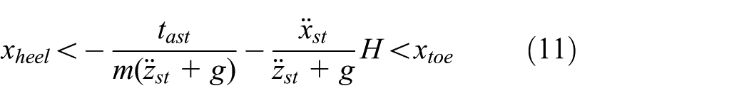
Then, the value range of stance torque $t_{\mathrm{ast}}$ is as follows

$$\begin{array}{c}-m({\stackrel{··}{z}}_{\mathrm{st}}+g)x_{\mathrm{toe}}-\mathrm{mH}{\stackrel{··}{x}}_{\mathrm{st}}<t_{\mathrm{ast}}\hfill \\ <-m({\stackrel{··}{z}}_{\mathrm{st}}+g)x_{\mathrm{heel}}-\mathrm{mH}{\stackrel{··}{x}}_{\mathrm{st}}\sqrt{a^2+b^2}\hfill \end{array}$$

(12)

The values of body horizontal acceleration ${\stackrel{··}{x}}_{\mathrm{st}}$ and vertical acceleration ${\stackrel{··}{z}}_{\mathrm{st}}$ are determined by an acceleration sensor. Equations (5) and (12) are the dynamic equations for the FIPM.

Control algorithm

Dynamic balance control idea

According to Newton’s second law of motion, force is the reason that an object’s motion changes. Disturbance forces such as an unexpected push from the outside world, an uneven ground, or an active push from itself will inevitably change its body’s motion. Figure 2 shows the relationship between a disturbance force and the FIPM body’s motion states. In this article, the dynamic balance control idea is servoing the body’s motion states within the desired targets in order to balance the disturbance forces. If the body encounters a disturbance force, its motion must change; the control algorithm monitors the body’s motion and corrects it when it deviates from the desired targets, neutralizing the disturbing force. The body’s motion states are controlled across its all freedoms, through the body height $z_{\mathrm{st}}$ for vertical freedom, the body pitch angle ${\theta }_b$ for rotational freedom, and the body level velocity ${\stackrel{·}{x}}_{\mathrm{st}}$ for horizontal freedom. Figure 3 shows the relationship between the legs’ actions and body’s motion. The body height $z_{\mathrm{st}}$ is controlled by the stance leg length $l_{\mathrm{st}}$ , the body pitch angle ${\theta }_b$ is controlled by the stance hip torque $t_{\mathrm{hst}}$ , and the body velocity ${\stackrel{·}{x}}_{\mathrm{st}}$ is controlled by the stance ankle torque $t_{\mathrm{ast}}$ and the swing foot placement $x_{\mathrm{sw}}$ for touchdown. The following subsections describe the concrete control algorithm.

Figure 2.

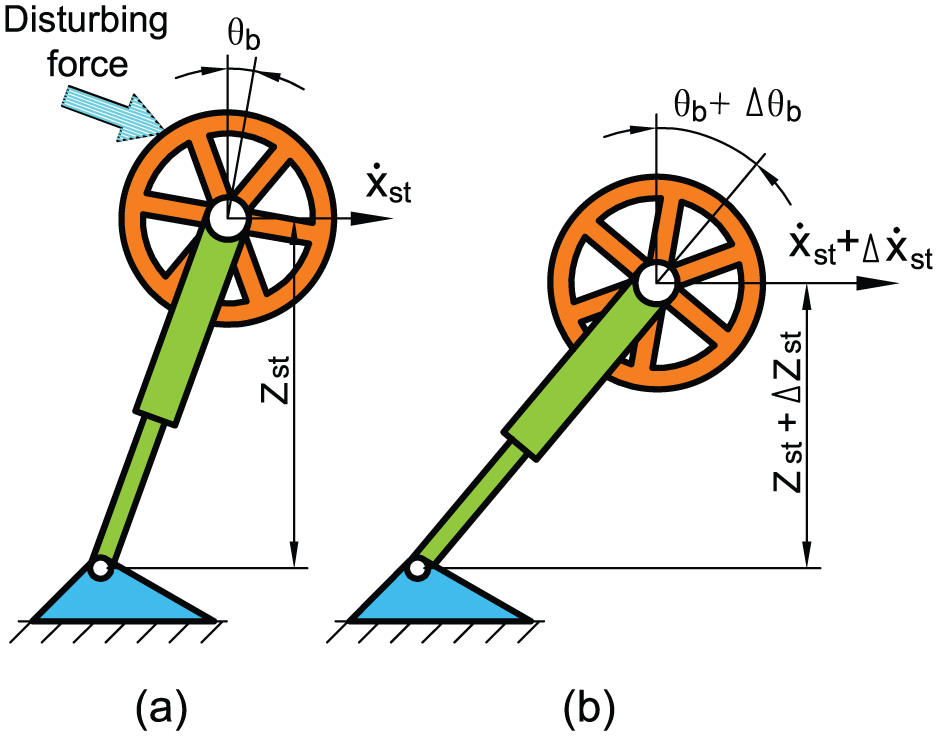
Relationship between disturbing force and body motion states: (a) the model’s motion states just before encountering a disturbing force and (b) the model’s motion states just after encountering a disturbing force.

Figure 3.

The corresponding control relation between the legs’ actions and the body motions based on the FIPM.

Servo body height $z_{\mathrm{st}}$

In Figure 1, the stance leg length $l_{\mathrm{st}}$ has the following relationship with body height $z_{\mathrm{st}}$

$$l_{\mathrm{st}}=\frac{z_{\mathrm{st}}}{\cos {\theta }_{\mathrm{lst}}}$$

(13)

When body height $z_{\mathrm{st}}$ remains constant, no energy is lost theoretically when swing leg touches down, ¹⁷ and linear items in dynamic equations ²⁰ make the control simpler. Therefore, the desired body height remains constant in our control algorithm as follows

$$z_{\mathrm{st}}=z_0$$

(14)

where $z_0$ is a constant value.

If the body height maintains a constant value $z_0$ , substituting $z_{\mathrm{st}}=z_0$ and ${\stackrel{··}{z}}_{\mathrm{st}}={\stackrel{·}{z}}_{\mathrm{st}}=0$ into equations (5) and (12) yields the new dynamic equations for the FIPM as follows

$$\{\begin{array}{c}m{\stackrel{··}{x}}_{\mathrm{st}}=\frac{\mathrm{mg}}{z_0}{x}_{\mathrm{st}}+\frac{1}{z_0}(t_{\mathrm{ast}}-t_{\mathrm{hst}})\hfill \\ m{\stackrel{··}{z}}_{\mathrm{st}}=0\hfill \\ J{\stackrel{··}{\theta }}_b=t_{\mathrm{hst}}\hfill \end{array}$$

(15)

and

$$-\mathrm{mg}{x}_{\mathrm{toe}}-\mathrm{mH}{\stackrel{··}{x}}_{\mathrm{st}}<t_{\mathrm{ast}}<-\mathrm{mg}{x}_{\mathrm{heel}}-\mathrm{mH}{\stackrel{··}{x}}_{\mathrm{st}}$$

(16)

Servo body pitch angle ${\theta }_b$

Because $J{\stackrel{··}{\theta }}_b=t_{\mathrm{hst}}$ is part of equation (15), the stance hip torque $t_{\mathrm{hst}}$ can be used to control body pitch angle ${\theta }_b$ by a proportional-derivative servo in equation (17). Figure (4) shows the control block of body pitch ${\theta }_b$

$$t_{\mathrm{hst}}=k_p({\theta }_b^d-{\theta }_b)+k_d(0-{\stackrel{·}{\theta }}_b)$$

(17)

Figure 4.

The control block of body pitch ${\theta }_b$ .

The closed-loop transfer function for controlling body pitch angle ${\theta }_b$ is as follows

$$\frac{{\theta }_b}{{\theta }_b^d}=\frac{k_p+k_{d}s}{J{s}^2+k_{d}s+k_p}$$

(18)

In biped walking, the expected body pitch angle ${\theta }_b^d$ is set to a constant value, so ${\stackrel{·}{\theta }}_b^d=0$ which means that $s{\theta }_b^d=0$ in the transfer function. Therefore, the closed-loop transfer function for controlling body pitch angle ${\theta }_b$ can be rewritten as follows

$$\frac{{\theta }_b}{{\theta }_b^d}=\frac{k_p}{J{s}^2+k_{d}s+k_p}=\frac{\frac{k_p}{J}}{s^2+\frac{k_d}{J}s+\frac{k_p}{J}}$$

(19)

By setting $\xi =k_d/2\sqrt{J{k}_p}$ and ${\omega }_n=\sqrt{k_p/J}$ , the transfer function can be converted as follows

$$\frac{{\theta }_b}{{\theta }_b^d}=\frac{{\omega }_n^2}{s^2+2\xi {\omega }_{n}s+{\omega }_n^2}$$

(20)

The transfer function for controlling body pitch angle is a standard two-order control system; when the damping coefficient $\xi$ and frequency ${\omega }_n$ are given, the coefficients $k_p$ and $k_d$ can be determined.

Servo body velocity ${\stackrel{·}{x}}_{\mathrm{st}}$

Based on the FIPM, the body velocity ${\stackrel{·}{x}}_{\mathrm{st}}$ is controlled not only by swing foot touchdown position $x_{\mathrm{sw}}$ but also by stance ankle torque $t_{\mathrm{ast}}$ .

Stance ankle torque $t_{\mathrm{ast}}$

The formula for controlling body velocity ${\stackrel{·}{x}}_{\mathrm{st}}$ through stance ankle torque $t_{\mathrm{ast}}$ can be obtained from the equation $m{\stackrel{··}{x}}_{\mathrm{st}}=(\mathrm{mg}/z_0)x_{\mathrm{st}}+(1/z_0)(t_{\mathrm{ast}}-t_{\mathrm{hst}})$ in equation (15) as follows

$$\begin{array}{c}m{\stackrel{··}{x}}_{\mathrm{st}}=\frac{\mathrm{mg}}{z_0}{x}_{\mathrm{st}}+\frac{1}{z_0}(t_{\mathrm{ast}}-t_{\mathrm{hst}})\hfill \\ \multicolumn{1}{c}{\Rightarrow t_{\mathrm{ast}}=t_{\mathrm{hst}}-\mathrm{mg}{x}_{\mathrm{st}}+m{z}_0{\stackrel{··}{x}}_{\mathrm{st}}}\\ \multicolumn{1}{c}{\Rightarrow t_{\mathrm{ast}}\approx t_{\mathrm{hst}}-\mathrm{mg}{x}_{\mathrm{st}}+m{z}_0\frac{\mathrm{\Delta }{\stackrel{·}{x}}_{\mathrm{st}}}{\mathrm{\Delta }T}}\\ \multicolumn{1}{c}{\Rightarrow t_{\mathrm{ast}}\approx t_{\mathrm{hst}}-\mathrm{mg}{x}_{\mathrm{st}}+\frac{m{z}_0}{\mathrm{\Delta }T}({\stackrel{·}{x}}_{\mathrm{st}}^d-{\stackrel{·}{x}}_{\mathrm{st}})}\end{array}$$

(21)

Setting $k=m{z}_0/\mathrm{\Delta }T$ yields the following

$$t_{\mathrm{ast}}=t_{\mathrm{hst}}-\mathrm{mg}{x}_{\mathrm{st}}+k({\stackrel{·}{x}}_{\mathrm{st}}^d-{\stackrel{·}{x}}_{\mathrm{st}})$$

(22)

Equation (22) and the ankle torque value range in equation (16) are servo formulas used to control body velocity ${\stackrel{·}{x}}_{\mathrm{st}}$ by stance ankle torque $t_{\mathrm{ast}}$ .

Swing foot touchdown position $x_{\mathrm{sw}}$

To establish the equation of the swing foot balance method, some simplifications are necessary. The effect of ankle torque $t_{\mathrm{ast}}$ and the hip torque $t_b$ are omitted. Therefore, the equation $m{\stackrel{··}{x}}_{\mathrm{st}}=(\mathrm{mg}/z_0)x_{\mathrm{st}}+(1/z_0)(t_{\mathrm{ast}}-t_{\mathrm{hst}})$ in equation (15) can be changed as follows

$${\stackrel{··}{x}}_{\mathrm{st}}=\frac{g}{z_0}{x}_{\mathrm{st}}$$

(23)

According to the linear IPM proposed by Kajita and Tani, ²⁰ if the swing foot position $x_{\mathrm{sw}}$ is equal to the stance foot position $x_{\mathrm{st}}$ at touchdown, the body’s average velocity will remain unchanged. ²⁰ This situation, shown in Figure 5(a), is called neutral point. If swing foot position $x_{\mathrm{sw}}$ is less than at the neutral point, the body’s velocity will increase, as shown in Figure 5(b). If swing foot position $x_{\mathrm{sw}}$ is greater than at the neutral point, the body’s velocity will decrease, as shown in Figure 5(c). The swing foot touchdown position deviates from neutral point in a nonlinear relation as the body’s velocity changes. In this article, we use a proportional-derivative servo to approximate this relationship, such that the formula for the swing foot balance method can be expressed as follows

$$x_{\mathrm{sw}}=x_{\mathrm{st}}+k_p({\stackrel{·}{x}}_{\mathrm{st}}^d-{\stackrel{·}{x}}_{\mathrm{st}})+k_i\sum ({\stackrel{·}{x}}_{\mathrm{st}}^d-{\stackrel{·}{x}}_{\mathrm{st}})$$

(24)

where ${\stackrel{·}{x}}_{\mathrm{st}}^d$ is the expected body velocity.

Figure 5.

Relationship between swing foot position and the body velocity change for linear inverted pendulum model: (a) unchanged, (b) increase, and (c) decrease.

Equations (22) and (24) are combined to servo the body velocity ${\stackrel{·}{x}}_{\mathrm{st}}$ .

Step frequency control

In a fixed leg-length inverted pendulum, the swing leg touches down as the body moves downward, and the swing leg lifts off the ground when the body moves upward. In contrast, in the linear IPM, the body height theoretically maintains a constant height $z_0$ , so the swing leg must actively lift up or touchdown. The control algorithm in this study is designed so that as the body moves away from the supporting point, the swing foot moves downward at a constant velocity ${\stackrel{·}{z}}_{\mathrm{sw}}$ until the other foot lifts off. As the body moves toward the supporting point, the swing foot moves upward at a constant velocity ${\stackrel{·}{z}}_{\mathrm{sw}}$ until the swing foot reaches a certain height $z_{\mathrm{sw}0}$ . One single step is composed of the swing foot’s lifting up and touchdown; therefore, the frequency $f_{\mathrm{step}}$ of one step is as follows

$$f_{\mathrm{step}}=\frac{1}{T_{\mathrm{step}}}=\frac{{\stackrel{·}{z}}_{\mathrm{sw}}}{2z_{\mathrm{sw}0}}$$

(25)

where $T_{\mathrm{step}}$ is the time from leg lift-off to leg touchdown.

When the step frequency $f_{\mathrm{step}}$ is given, the swing foot’s vertical velocity ${\stackrel{·}{z}}_{\mathrm{sw}}$ can be deduced as follows

$${\stackrel{·}{z}}_{\mathrm{sw}}=2z_{\mathrm{sw}0}{f}_{\mathrm{step}}$$

(26)

The swing foot’s vertical velocity ${\stackrel{·}{z}}_{\mathrm{sw}}$ can be determined by the step frequency precise in smooth ground and coarse in the unknown rough ground. If the biped walking occurs on an unknown rough ground, the swing leg’s height may be different to the stance leg’s when touchdown for maintaining body height is unchanged, as well as in dual length linear inverted pendulum mode (DLLIPM). ²¹

Comparative analysis in phase-plane

This section will analyze the foot’s effect in phase-plane. The biped’s passive dynamic motion in the phase-plane is given first, and then compares the biped motion in phase-plane when based on the IPM and the FIPM. The biped based on the IPM can balance disturbance through the swing foot touchdown $x_{\mathrm{sw}}$ , and the biped based on the FIPM can balance disturbance through both swing foot touchdown $x_{\mathrm{sw}}$ and stance ankle torque $t_{\mathrm{ast}}$ .

The phase-plane

Phase-plane analysis of biped passive dynamic motion

The phase-plane expresses the biped motion process on a plane using body level displacement $x_{\mathrm{st}}$ and body level velocity ${\stackrel{·}{x}}_{\mathrm{st}}$ as coordinates. Body pitch angle ${\theta }_b$ and stance hip torque $t_{\mathrm{hst}}$ have no special effect in the two models, so rotating freedoms are omitted in the IPM and the FIPM for simplicity’s sake. If the biped moves by a passive dynamic, stance ankle torque $t_{\mathrm{ast}}$ and swing foot displacement $x_{\mathrm{sw}}$ are disabled; in that case, equation (15) can be reduced as follows

$$m{\stackrel{··}{x}}_{\mathrm{st}}=\frac{\mathrm{mg}}{z_0}{x}_{\mathrm{st}}$$

(27)

Integrating the two sides yields the following

$$\frac{1}{2}{\stackrel{·}{x}}_{\mathrm{st}}^2=\frac{g}{2z_0}{x}_{\mathrm{st}}^2+E$$

(28)

where E is a constant.

Equation (28) is composed of g, $z_0$ , body level displacement $x_{\mathrm{st}}$ , the body level velocity ${\stackrel{·}{x}}_{\mathrm{st}}$ , and a constant value E. Gravity acceleration g is 9.8 m/s² and the linear inverted pendulum height $z_0$ is 0.7 m in our biped robot. If E is defined, the phase-plane can be obtained through equation (28). In order to observe the motion characteristics, E is randomly set at 0, ±0.3, ±0.6 and ±0.9, producing a set of curves in the phase-plane in Figure 6. The phase plot can be divided into four quadrants: I, II, III, and IV. In quadrants II and IV, the IPM is moving toward the supporting point, meaning that it is increasing. In quadrants I and III, the IPM is moving away the supporting point, meaning that it is decreasing. Figure 6 demonstrates that if the linear inverted pendulum is in quadrants II and IV, it will move into quadrants II and IV finally and could not be back again. Whatever state the passive linear inverted pendulum is in, it will ultimately fall down.

Figure 6.

Phase-plane of passively moving biped robot.

Phase-plane analysis of IPM

If a biped’s balance is based on the IPM, swing foot placement $x_{\mathrm{st}}$ can be used to regulate biped motion. In that case, the dynamic equation can be expressed as follows

$$\{\begin{array}{c}{\stackrel{··}{x}}_{\mathrm{st}}=\frac{g}{z_0}{x}_{s{t}^{-}}\mathrm{Before}\mathrm{touchdown}\hfill \\ {\stackrel{··}{x}}_{\mathrm{st}}=\frac{g}{z_0}{x}_{s{t}^{+}}\mathrm{After}\mathrm{touchdown}\hfill \end{array}$$

(29)

where $x_{s{t}^{-}}$ is stance foot horizontal position before touchdown and $x_{s{t}^{-}}$ is the stance foot horizontal position after touchdown.

Phase-plane analysis of the FIPM

If a biped’s balance is based on the FIPM, both the swing foot placement $x_{\mathrm{st}}$ and the stance ankle torque $t_{\mathrm{ast}}$ can be used to regulate biped motion. In that situation, the biped’s dynamic equation can be expressed as follows

$$\{\begin{array}{cc}{\stackrel{··}{x}}_{\mathrm{st}}=\frac{g}{z_0}(x_{s{t}^{-}}+\mathrm{\Delta }{x}_{s{t}^{-}})\hfill & \mathrm{Before}\mathrm{touchdown}\hfill \\ \multicolumn{1}{c}{{\stackrel{··}{x}}_{\mathrm{st}}=\frac{g}{z_0}(x_{s{t}^{+}}+\mathrm{\Delta }{x}_{s{t}^{+}})}& \mathrm{After}\mathrm{touchdown}\hfill \end{array}$$

(30)

where $\mathrm{\Delta }{x}_{s{t}^{-}}$ is stance foot ZMP position before touchdown and $\mathrm{\Delta }{x}_{s{t}^{-}}$ is the stance foot ZMP position after touchdown.

Comparing balancing abilities in the phase-plane

For the comparative analysis, we simulated both of the models. The energy E is set to zero to begin with, and the control target was keeping the biped stopped over the supporting point. In this process, the biped undergoes three disturbances occurring at point A, D, and O. The disturbance at point A makes the biped’s velocity suddenly increase 0.29 m/s, the disturbance at point F makes the biped’s velocity suddenly increase 0.12 m/s, and the disturbance at point O makes the biped’s velocity suddenly increase 0.08 m/s. Figure 7 shows the biped’s motion process for different models in phase-plane. Figure 7(a) represents the motion phase plot based on the IPM, and Figure 7(b) represents the motion phase plot based on the FIPM.

Figure 7.

Biped motion process based on the IPM and FIPM in the phase-plane.

When the biped experiences a large unexpected disturbance at Point A, its velocity suddenly increases about 0.29 m/s, raising the biped’s orbit energy E up to 0.1. Based on the IPM, according to equation (29), the body’s dynamic equation can actively change when the swing leg touches down. The biped moves passively along the curve BC in the orbit energy E = 0.1 before touchdown in Figure 7(a); then the swing leg’s touchdown instantaneously converts the biped’s motion state from point C to point D, and after touchdown, it will again move passively along the orbit energy curve E = 0. Based on the FIPM, according to equation (30), the body’s dynamic equation can actively change not only through swing leg’s touchdown, but also by adjusting stance foot’s ZMP via stance ankle torque $t_{\mathrm{ast}}$ . The biped’s motion state is first adjusted by the stance foot’s ZMP before swing leg touches down, changing the biped motion state from point B to point C and decreasing the biped’s orbit energy E from 0.1 to 0.05 as shown in Figure 7(b). However, the disturbance is too large for the limited foot length, and the biped’s orbit energy cannot recover to 0 by adjusting the stance foot’s ZMP; therefore, the biped passively moves along the curve CC′ at the orbit energy E = 0.05 as shown in Figure 7(b). The swing leg’s touchdown instantaneously changes the biped’s motion state from point C′ to point D, and it moves passively along the orbit energy curve E = 0 again after touchdown. When suffering a larger disturbance, the biped based on the IPM uses the swing foot’s touchdown for balance, while the biped based on the FIPM simultaneously uses both the swing foot’s touchdown and the stance ankle’s torque for balance.

When the biped experiences a smaller unexpected disturbance at Point F, the biped’s velocity suddenly increases about 0.12 m/s, raising the orbit energy E up to 0.03. Based on the IPM, according to equation (29), the biped uses the swing leg’s touchdown for balance, similar to the reaction to a larger disturbance at point A. Based on the FIPM, according to equation (30), the biped’s motion state is adjusted by stance foot ZMP, which converts the biped motion state from point G to point H and converts the biped’s orbit energy E from 0.03 to 0. In this way, the disturbance is balanced by adjusting the stance foot ZMP in single stance phase before the swing leg touches down. When experiencing a smaller disturbance, the biped based on IPM uses the swing foot’s touchdown for balance, while the biped based the FIPM uses only stance ankle’s torque for balance in single leg stance phase. Therefore, the biped based on the FIPM can more quickly balance small disturbances than the biped based on the IPM.

When the biped reaches the critical steady point O, it can fall down forward or backward because of smaller random disturbance. Without a loss of generality, suppose that a small random disturbance causes a sudden increase in the biped’s velocity of 0.08 m/s. The disturbance changes the body’s motion state from point O to point P, and the orbit energy changes from 0 to 0.003. According to equation (29), the biped based on the IPM moves passively along the orbit energy curve E = 0.003 before the swing leg touches down; as shown in Figure 7(a), the swing leg’s touchdown changes the biped’s motion state moving from point Q to R, reducing the orbit energy to just below 0 for guaranteeing the biped motion reverted. Then the biped moves passively along the curve RS at orbit energy E = −0.003 until the swing leg touches down again. The biped will constantly move forward and backward along circle RSTU, moving about 0.2 m in the process. In this situation, the biped based on the IPM cannot remain in the stopping state. The biped based on the FIPM can balance the disturbance by adjusting stance foot ZMP. Although this adjusting process is similar to that based on the IPM, the adjustment by stance foot ZMP occurs instantaneous, more quickly than by swing foot touchdown, such that the biped based on the FIPM can keep stand still. This indicates that the biped based on the FIPM has the ability to stop itself.

Joint control of the biped robot

The previous sections describe the FIPM and its control methods. This section briefly introduces the biped robot, then discusses the forward kinematics and inverse kinematics relationships between the FIPM and the biped robot, and finally describes the joints control of the biped robot.

The biped robot

Figure 8 shows a solid model of the biped robot that weight 65 kg and has a height of 130 cm. The biped is composed of seven parts: one body, two thighs, two calves, and two feet. It has six freedoms: one hip joint, one knee joint, and one ankle joint for each leg. Each joint is driven by a hydraulic servo cylinder with force and displacement sensors. Two foot sensors are used to detect ground contact and one inertial sensor detect the body postures and accelerations. The biped robot performs planar motion with forward and vertical direction displacements and pitch rotation by an auxiliary bracket.

Figure 8.

Solid model of the biped robot.

The kinematics relations

Figure 9 shows the relationship between the inverted pendulum model and the biped robot.

Figure 9.

Relationship between (a) the inverted pendulum’s COM position and (b) the biped joints’ angles.

Forward kinematics involves deriving the COM position $(x,z)$ from $({\theta }_k,{\theta }_h,{\theta }_b)$ as follows

$$\{\begin{array}{c}x=l_h\sin {\theta }_b+l_t\sin ({\theta }_b+{\theta }_h)+l_c\sin ({\theta }_b+{\theta }_h+{\theta }_k)\hfill \\ \multicolumn{1}{c}{z=l_h\cos {\theta }_b+l_t\cos ({\theta }_b+{\theta }_h)+l_c\cos ({\theta }_b+{\theta }_h+{\theta }_k)}\end{array}$$

(31)

where $l_c$ is the length from ankle joint to knee joint, $l_t$ is the length from knee joint to hip joint, and $l_h$ is the length from hip joint to the COM.

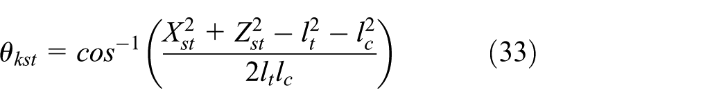
Inverse kinematics involves deriving the joint angle $({\theta }_k,{\theta }_h)$ from $(x,y,{\theta }_b)$ as follows

$$\{\begin{array}{c}{\theta }_k=\mathrm{co}{s}^{-1}\left(\frac{X^2+Z^2-l_t^2-l_c^2}{2l_t{l}_c}\right)\hfill \\ \multicolumn{1}{c}{{\theta }_h=t{g}^{-1}\left(\frac{\mathrm{BDcos}{\theta }_k+\mathrm{ADsin}{\theta }_k-\mathrm{BC}}{\mathrm{BDsin}{\theta }_k-\mathrm{ADcos}{\theta }_k+\mathrm{AC}}\right)}\end{array}$$

(32)

where $X=\mathrm{xcos}{\theta }_b-\mathrm{zsin}{\theta }_b$ , $Z=\mathrm{xsin}{\theta }_b+\mathrm{zcos}{\theta }_b-l_h$ , $A=X/\sqrt{X^2+Z^2}$ , $B=Z/\sqrt{X^2+Z^2}$ , $C=(X^2+Z^2+l_c^2-l_t^2)/2l_c\sqrt{X^2+Z^2}$ , and $D=(X^2+Z^2+l_t^2-l_c^2)/2l_t\sqrt{X^2+Z^2}$ .

Joint control

The biped has six joints that need to be controlled: two hip joints, two knee joints, and two ankle joints. The hip, knee, and ankle joint of stance leg are called the stance hip, stance knee, and stance ankle. The hip, knee, and ankle joint of swing leg are called the swing hip, swing knee, and swing ankle.

The stance hip controls body pitch angle ${\theta }_b$ through its torque $t_{\mathrm{hst}}$ as determined by equation (17).

The stance knee joint controls body height $z_{\mathrm{st}}$ by its angle ${\theta }_{\mathrm{kst}}$ which can be deduced from equation (32) as follows

$${\theta }_{\mathrm{kst}}=\mathrm{co}{s}^{-1}\left(\frac{X_{\mathrm{st}}^2+Z_{\mathrm{st}}^2-l_t^2-l_c^2}{2l_t{l}_c}\right)$$

(33)

where $X_{\mathrm{st}}=x_{\mathrm{st}}\cos {\theta }_b-z_0\sin {\theta }_b$ and $Z_{\mathrm{st}}=x_{\mathrm{st}}\sin {\theta }_b+z_0\cos {\theta }_b-l_h$ .

The stance ankle controls body velocity ${\stackrel{·}{x}}_{\mathrm{st}}$ through its torque $t_{\mathrm{ast}}$ which is determined by equation (22).

Swing hip angle ${\theta }_{\mathrm{hsw}}$ and swing knee angle ${\theta }_{\mathrm{ksw}}$ control body velocity ${\stackrel{·}{x}}_{\mathrm{st}}$ by swing foot placement position $x_{\mathrm{sw}}$ and $z_{\mathrm{sw}}$ , and swing hip and swing knee angles are expressed as follows

$${\theta }_{\mathrm{ksw}}=\mathrm{co}{s}^{-1}\left(\frac{X_{\mathrm{sw}}^2+Z_{\mathrm{sw}}^2-l_t^2-l_c^2}{2l_t{l}_c}\right)$$

(34)

$${\theta }_{\mathrm{hsw}}=t{g}^{-1}\left(\frac{B_{\mathrm{sw}}{D}_{\mathrm{sw}}\cos {\theta }_k+A_{\mathrm{sw}}{D}_{\mathrm{sw}}\sin {\theta }_k-B_{\mathrm{sw}}{C}_{\mathrm{sw}}}{B_{\mathrm{sw}}{D}_{\mathrm{sw}}\sin {\theta }_k-A_{\mathrm{sw}}{D}_{\mathrm{sw}}\cos {\theta }_k+A_{\mathrm{sw}}{C}_{\mathrm{sw}}}\right)$$

(35)

where

$$\begin{array}{c}{X}_{\mathrm{sw}}=x_{\mathrm{sw}}\cos {\theta }_b-z_{\mathrm{sw}}\sin {\theta }_b\hfill \\ Z_{\mathrm{sw}}=x_{\mathrm{sw}}\sin {\theta }_b+z_{\mathrm{sw}}\cos {\theta }_b-l_h\hfill \\ A_{\mathrm{sw}}=\frac{X_{\mathrm{sw}}}{\sqrt{X_{\mathrm{sw}}^2+Z_{\mathrm{sw}}^2}}\hfill \\ B_{\mathrm{sw}}=\frac{Z_{\mathrm{sw}}}{\sqrt{X_{\mathrm{sw}}^2+Z_{\mathrm{sw}}^2}}\hfill \\ C_{\mathrm{sw}}=\frac{X_{\mathrm{sw}}^2+Z_{\mathrm{sw}}^2+l_c^2-l_t^2}{2l_c\sqrt{X_{\mathrm{sw}}^2+Z_{\mathrm{sw}}^2}}\hfill \\ D_{\mathrm{sw}}=\frac{X_{\mathrm{sw}}^2+Z_{\mathrm{sw}}^2+l_t^2-l_c^2}{2l_t\sqrt{X_{\mathrm{sw}}^2+Z_{\mathrm{sw}}^2}}\hfill \end{array}$$

In order to calculate ${\theta }_{\mathrm{hsw}}$ and ${\theta }_{\mathrm{ksw}}$ , body pitch angle ${\theta }_b$ and swing foot position $x_{\mathrm{sw}}$ and $z_{\mathrm{sw}}$ are required. The body pitch angle is detected by inertia sensor, swing foot position $x_{\mathrm{sw}}$ is determined by equation (24), and the swing foot position in vertical direction $z_{\mathrm{sw}}$ is calculated by forward kinematics in equation (31).

The torque of the swing ankle is set to zero as follows

$$t_{\mathrm{asw}}=0$$

(36)

Equations (17), (22), and (33)–(36) are used to control the biped robot’s six joints.

Experiment and results

Figure 10 shows the experiment’s control process. The controller reads the sensors’ data including body pitch ${\theta }_b$ , stance hip angle ${\theta }_{\mathrm{hst}}$ , and stance knee angle ${\theta }_{\mathrm{kst}}$ , then converts the data into the parameter $x_{\mathrm{st}}$ of the inverted pendulum through forward kinematics equation (31). The controller then applies the FIPM’s control algorithm through equations (14), (17), (22), and (24) and converts the FIPM control into the biped’s joint control through equations (33)–(35). In this experiment, the control process is executed at 1000 Hz.

Figure 10.

Experimental control process.

This section describes two experiments performed according to the same control program. One experiment changed the body expected velocity $v_d$ by remote controller, verifying the effectiveness of the three-decomposition control algorithm based on the FIPM. The other experiment maintained the body velocity $v_d$ at zero and introduced an unexpected impact to verify the dynamic balancing ability of the control algorithm based on the FIPM.

Velocity control test

In this experiment, the biped walked along the expected velocity. The body pitch angle ${\theta }_b$ and body height $z_{\mathrm{st}}$ influence swing foot displacement $x_{\mathrm{sw}}$ , and Figure 11 illustrates their relationship. Based on Figure 11(a), when the body pitch angle is 0 rad, the range $x_{\mathrm{sw}}$ is at its largest, from −200 to 200 mm; Therefore, this experiment sets the expected body pitch angle ${\stackrel{·}{\theta }}_b^d$ to 0 rad. Figure 11(b) shows that the range of $x_{\mathrm{sw}}$ is largest when the body height is just above 684 mm, and if the body height $z_0$ falls below 684 mm, the range of $x_{\mathrm{sw}}$ decreases sharply. Therefore, this experiment designated 700 mm as body height $z_0$ for safety, and the range of $x_{\mathrm{sw}}$ was from −200 to 200 mm. The expected body velocity was set by remote controller.

Figure 11.

Swing foot position $x_{\mathrm{sw}}$ range relationship to (a) body pitch ${\theta }_b$ angle and (b) body height $z_{\mathrm{st}}$ .

Figure 12 shows the data resulting from the experiment. The red dashed line stands for the expected value, and the blue solid line stands for the actual value. Figure 12(b) shows the biped’s velocity–time curve, demonstrating that on the whole, the actual body velocity can track the expected body velocity. Figure 12(c) shows the biped height–time curve; the actual body height was about 700 mm, with an error range of 5 mm. Figure 12(d) shows the biped’s pitch angle–time curve. The actual pitch angle has about 0.1 rad error in relation to the expect body pitch angle. The conclusions from Figure 12(b)–(d) can be summarized in one sentence: the body can move at a certain height with a certain body posture. Since the body is a part of robot, this means that the biped can move. Figure 12(a) shows the biped’s displacement–time curve; the displacement tracking error is about 0.1 m, which is acceptable. This experiment demonstrates that the biped can track the expected velocity using our three-decomposition control algorithm based on the FIPM.

Figure 12.

Experiment data on velocity control: (a) body moving distance, (b) body velocity, (c) body height, and (d) body pitch angle.

Anti-disturbance test

The dumbbell impulse experiment was used to analyze the biped’s dynamic balance using the control algorithm based on the FIPM. In this experiment, a dumbbell weighting 10 kg is hung just before the biped robot on a 0.85 m length rope. The dumbbell is first pulled up about 30° and then swings down freely because of gravity and hits the biped as it stepping on the ground. Figure 13 shows the time-elapse image sequence over the first 2 s of this experiment.

Figure 13.

Time-lapse sequence of the first 2 s.

Figure 14 shows the experimental data. Figure 14(a) shows the velocity–time curve, which indicates that the biped moves backward upon the dumbbell’s impact before returning automatically to its original position. The integrated expression for swing foot velocity in equation (24) stands for the displacement error, giving the biped the ability to correct itself. Figure 14(b) shows the biped’s velocity–time curve. The expected body velocity ${\stackrel{·}{x}}_{\mathrm{st}}^d$ is 0 m/s, meaning that it is stepping on the ground. The body velocity curve features waves; if the wave period is clearly smaller than a single-step period, it is produced by stance ankle torque $t_{\mathrm{ast}}$ . Equation (22) shows that the stance ankle torque is proportionally related to the velocity error. If the wave period is close to a single-step period, it is produced by swing foot touchdown. Figure 14(c) shows the stance foot ZMP–time curve, adapted from equation (9) by substituting the experimental data. When the ZMP equals 0, the foot has no contribution for biped walking. When the ZMP is negative, the foot is accelerating the biped, and when the ZMP is positive, the foot is decelerating the biped. The curves show that the stance foot ZMP fluctuates continuously in a range of about ±50 mm. Figure 14(d) shows the error between two foot positions when the swing foot touches down. When the error is zero, the body velocity is unchanged. When two foot position error is negative, the biped accelerates, and when the error is positive, the biped decelerates. Because swing foot balance method takes action only when it touches down, the curve consists of a set of discrete points. The curve shows that the two foot position error is nearly 100 mm when the dumbbell makes its impact, which is more than the ZMP wave of 50 mm; this indicates that the swing foot touchdown takes greater action when suffering a larger disturbance. When the biped experiences a small disturbance, the two foot position error at touchdown is similar to stance foot ZMP. However, adjusting the stance foot ZMP is a continuous process, such that the stance foot plays a major role when small disturbances occur.

Figure 14.

Experimental data for anti-disturbance test: (a) body moving distance, (b) body velocity, (c) zero moment point of stance foot, and (d) the position error between two feet.

Disturbance is existed in various other manners besides dumbbell impacting. Hand pushing and foot kicking are common disturbances in our surroundings. Although walking on complex ground can be seen as ground adaptability, it is a disturbance essentially for biped walking because the complex ground will disturb the body motion states finally. For testing anti-disturbance ability enough, the tests including handing pushing, foot kicking, and walking on snow ground and on stone ground are done. The experiment screenshots are shown in Figure 15, and these experiments showed that the biped can balance these disturbances as well as balancing dumbbell impacting.

Figure 15.

The rough ground composed by stone and sand: (a) hand push, (b) foot kick, (c) snow ground, and (d) stone ground.

Conclusion

This article proposes a FIPM, in which the biped’s velocity is controlled not only by swing foot placement, but also by stance ankle. A three-decomposition control algorithm for biped walking is created based on the FIPM. The results show that the biped can endure larger disturbances and response quickly to small disturbances, meaning that it has good dynamic balance and stopping ability, which are important requirements for practical use. The control algorithm is simple and performs well, and it can be used to control a biped walking in a less complicated way than existing methods allow.