
Abstract
The transfer matrix method for multibody systems has been developed for 20 years and improved constantly. The new version of transfer matrix method for multibody system and the automatic deduction method of overall transfer equation presented in recent years make it more convenient of the method for engineering application. In this article, by first defining branch subsystem, any complex multibody system may be regarded as the assembling of branch subsystems and simple chain subsystems. If there are closed loops in the system, the loops should be “cut off,” thus a pair of “new boundaries” are generated at each “cutting-off” point. The relationship between the state vectors of the pair of “new boundaries” may be described by a supplement equation. Based on above work, the automatic deduction method of overall transfer equation for tree systems as well as closed-loop-and-branch-mixed systems is formed. The results of numerical examples obtained by the automatic deduction method and ADAMS software for tree system dynamics as well as mixed system dynamics have good agreements, which validate the features of proposed method such as high computational speed, more effective for complex systems, no need of the system global dynamics equation, highly programmable, as well as convenient popularization and application in engineering.
Keywords
Introduction
Multibody system dynamics methods (MSDMs) that have been developed since 50 years ago1–7 provide effective methods for dynamics analysis of modern mechanical systems. Consequently, the developments of ships, aircraft, aerospace, traffics, and general machinery industry have been promoted greatly. The main study object of MSDM is the system composed of multiple bodies with relative movements. Establishment of the global dynamics equation of system and its numerical computation are the most important tasks of ordinary MSDM. Meanwhile, improving the speed, precision, and stability of the numerical computation are the key study contents.
With the development and demand of engineering technology, mechanics researchers worldwide are making their effort to present and improve various MSDM creatively. Despite various ordinary MSDMs have different styles, they have two identical features: (1) it is necessary to establish the system global dynamics equation, which is the most brilliant but the most difficult part for each MSDM. (2) For a complex system, the system matrix order of the global dynamics equation is very high. Therefore, it is one of the most important study directions to find effective ways to reduce the order of the system matrix for overcoming the computational difficulty.
For improving the computational speed and simplifying the study procedure of multibody system dynamics (MSD), a lot of researchers have been devoted in developing kinds of algorithms based on classical MSDM. From 1980s to 1990s was the period of rapid development of MSDM. The algorithms proposed by Featherstone,
8
Brandl et al.,
9
Rodriguez et al.,
10
Saha
11
are all efficient for the number of operations and the storage requirements of these algorithms are proportional to the degrees of freedom of multibody system. The common features of these algorithms are (1) no need to establish the global system dynamics equation and (2) usage of recursive thoughts. According to Featherstone,
8
Brandl et al.
9
and Saha,
11
the relationship of computational complexities of these algorithms is Saha
11
> Featherstone
8
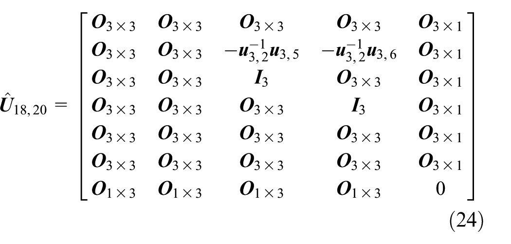
> Brandl et al.,
9
which shows that the algorithm by Brandl is the most efficient. Even though the algorithm by Saha is worse than that by Featherstone
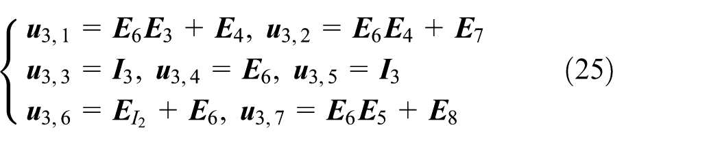
8
in terms of the complexities, it provides a simpler algorithm, which is easier to implement. Transfer matrix method for multibody system (MSTMM) was developed for the exact target with above algorithms. Rui and colleagues12–19 have put forward MSTMM and tried to perfect it constantly since 20 years ago. The MSTMM has been applied widely in engineering for following aspects: the study procedure of MSD is simplified because of no need to establish the system global dynamics equation; the computational speed is increased greatly because the system matrix order is always low, and it is highly programmable. The new version of MSTMM
16
was presented in 2013, of which the computational complexity is in the order
The salient contributions of this article are as follows:
The branch subsystem is first defined.
The general formulae of transfer matrix and transfer equation for branch subsystems are derived, which simplifies the deduction process and the form of overall transfer equation for various complex multibody systems greatly. Thus, it becomes convenient to realize the automatic deduction of overall transfer equation for multibody systems with various complex topology graphs.
By “cutting off” the closed-loop subsystem, any closed-loop-and-branch-mixed systems may be regarded as a tree system with “new boundaries” generated at each “cutting-off” point.
The automatic deduction method of overall transfer equation for tree systems as well as closed-loop-and-branch-mixed systems is formed, which would provide theoretical support for the software development based on the new version of MSTMM.
Fundamentals of the new version of MSTMM
The basic idea of the new version of MSTMM is “to break up the whole into parts,” that is, to separate a complex multibody system into several body elements and hinge elements whose dynamics characteristics may be expressed by matrices. The transfer equations and transfer matrices of elements are deduced by their dynamics equations strictly. Building up the transfer equation and transfer matrix library of all kinds of elements in advance, the overall transfer matrix and the overall transfer equation of the system may be obtained by assembling them according to topology graph of the system easily. Next, boundary conditions and initial conditions may be utilized to solve the transfer equations of system and all elements, and then the state vectors on the boundaries and elements at present moment may be obtained. The displacement, velocity, rotation angle, angular velocity, and other system motion characteristics at next moment may be determined by numerical integration methods. Thereby, the dynamics characteristics of the system may be gained. Especially for a chain system, the overall transfer matrix can be obtained by successively multiplying transfer matrices of all elements of the system.12,16
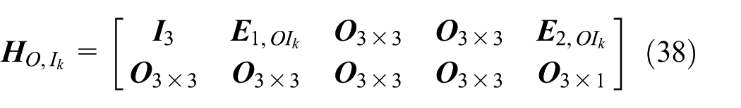
Coordinate system and direction cosine matrix
As shown in Figure 1, the motion of a system is described in the global inertial coordinate system

Global inertial coordinate system
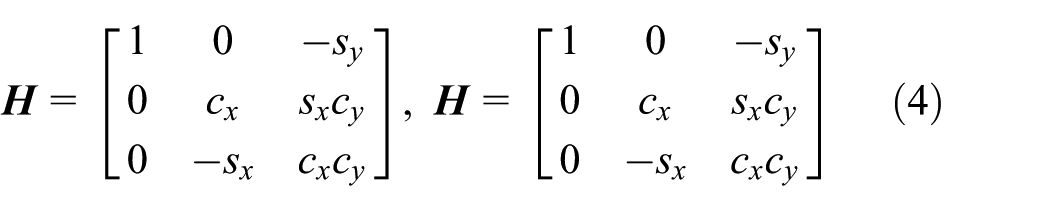
It has been proved 5 that the direction cosine matrix which transforms vectors in the body-fixed coordinates into the inertial coordinates is

where
The relationships among the absolute angular velocity


and

where
Substituting the derivative of equation (3) into equation (2b) yields

As long as the initial condition
Topology graph of MSD model and label convention
The topology graph of MSD model, as shown in Figure 2, is a new diagramming method for MSTMM to describe the transfer information. To be noted that in the topology graph, circles denote body elements (could be rigid bodies, beams, rods or other flexible bodies), while arrows denote hinge elements. 0 presents the boundary while the other numbers are the sequence number of elements. Usually, one boundary is chosen as the output of the whole system that is defined as root boundary while others are inputs as tip boundaries. Form tips to the root, the sequence numbers gradually increase.

Topology graph of a closed-loop-and-branch-mixed system.
Details about label convention are in Rui et al. 20
State vector, transfer matrix, and transfer equation
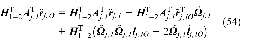
In the new version of MSTMM, the definitions of state vector, transfer matrix and transfer equation of elements, system overall transfer matrix and transfer equation as well as the principle for solution may be found in Rui et al.16,17 Here, only the expressions are given.
The state vector of elements with spatial motion is

where

For element

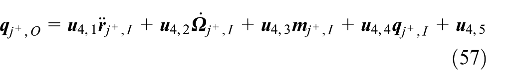
where
The overall state vector of system boundaries is
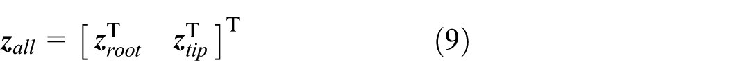
where
The overall transfer equation of system is

where
Transfer equations and transfer matrices of branch subsystems and typical elements
Definition of branch subsystems
The subsystem composed of a multi-input body and all inboard hinges of the body, as dashed part in Figure 3, is defined as a branch subsystem, where

Topology graph of a branch subsystem.
Transfer equation and geometric equation of branch subsystem
Transfer equation of a rigid body with multiple inputs and single output
According to the description in Rui et al.
20
, for a spatial motion body with multiple inputs and single output, like body

Similar to equation (8), the transfer equation of the spatial motion body with multiple inputs is

and its transfer matrix is 20

where


For rigid body 21 with two inputs and single output in Figure 2, the transfer equation and transfer matrix are


where the corresponding parameter matrices are defined in equations (14) and (15).
Transfer equation of multi-hinge subsystem
The concept of multi-hinge subsystem is first put forward in Rui et al.
20
, which is composed of multiple hinges those have the same outboard body, like
The multi-hinge subsystem composed of multiple smooth ball and socket hinges is taken as an example to demonstrate the transfer equation and transfer matrix of the multi-hinge subsystem. For each smooth ball-and-socket hinge
If the output of the outboard body also connects to a smooth ball-and-socket hinge, the main transfer equation 20 of multi-hinge subsystem is

where


where
For the multi-hinge subsystem composed by smooth ball-and-socket hinges 19 and 20 in Figure 2, the main transfer equation and associated transfer matrices are

where according to equation (17), the associated partition matrices are
Main transfer equation of branch subsystem
Based on equations (12) and (19), the main transfer equation of the branch subsystem in Figure 3 is

where
According to equation (26), for branch subsystem made up of rigid body 21, smooth ball-and-socket hinges 19 and 20 in Figure 2, the main transfer equation is
Geometric equations of branch subsystem
For a branch subsystem, only the main transfer equation is not enough to get the unknowns in the state vectors. Thus, it is necessary to introduce geometric equations. Geometric equation is used to describe the relationship of accelerations and internal moments between the output and non-first inputs in branch subsystem.
For the multi-input body

where

The relationship of acceleration between the first input

where

In equations (28)–(31),
For one smooth ball-and-socket hinge, the accelerations at input end and output end are equal, that is

where
Substituting equations (30) and (32) into equation (28) yields

where

Moreover, for an arbitrary smooth ball-and-socket hinge, the internal moments at inputs are zero, which may be expressed as

Therefore, rewriting equations (32) and (34) in the compact form yields the geometric equation of branch subsystem

where


where


Transfer equation and transfer matrix of typical elements
Spatial motion body with single input and single output
The transfer equation of spatial motion rigid body
The transfer matrix is 20

where

Spatial motion smooth ball-and-socket hinge
The transfer equation of smooth ball-and–socket hinge
The transfer matrix is 20

where
Spatial motion smooth sliding hinge
The transfer equation of smooth sliding hinge
For sliding hinge


where

The acceleration at output is

where


Taking the first and second time derivatives of equation (48) results in


The vectors in equation (52) are projected onto the body-fixed coordinate system as

Equation (53) includes three equations. Here, in order to eliminate the term of relative sliding acceleration, the first two equations are extracted
where

Assuming the output of the outboard body of the sliding hinge

According to the transfer equation of outboard body of the sliding hinge
where

Substituting equation (57) into equation (56), it becomes

Considering equations (45), (46a), (50), and (59) could be rewritten as

In view of equations (46b), (60) may be changed into

where

Rewriting equations (54) and (61) in a compact form yields

Based on the transfer equation of a sliding hinge

where
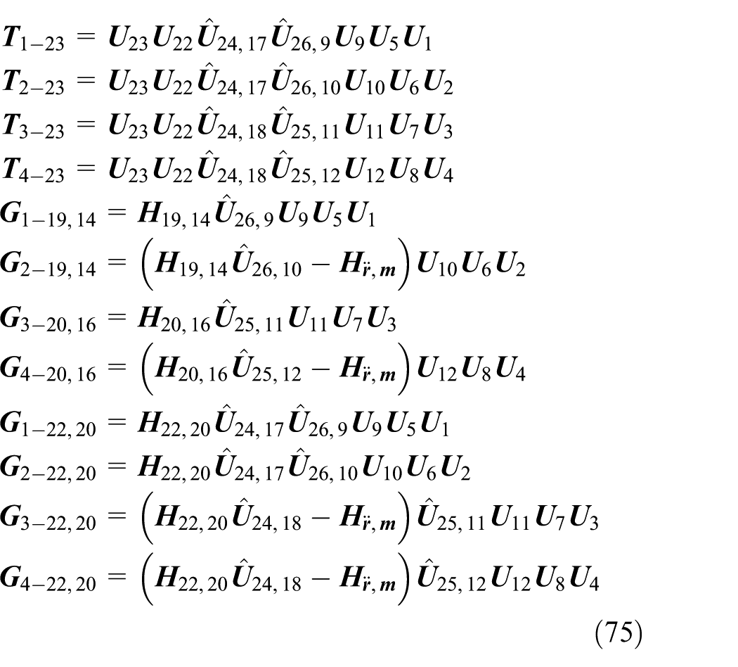
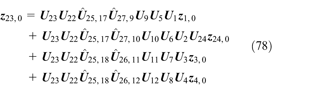
Overall transfer equation for tree systems
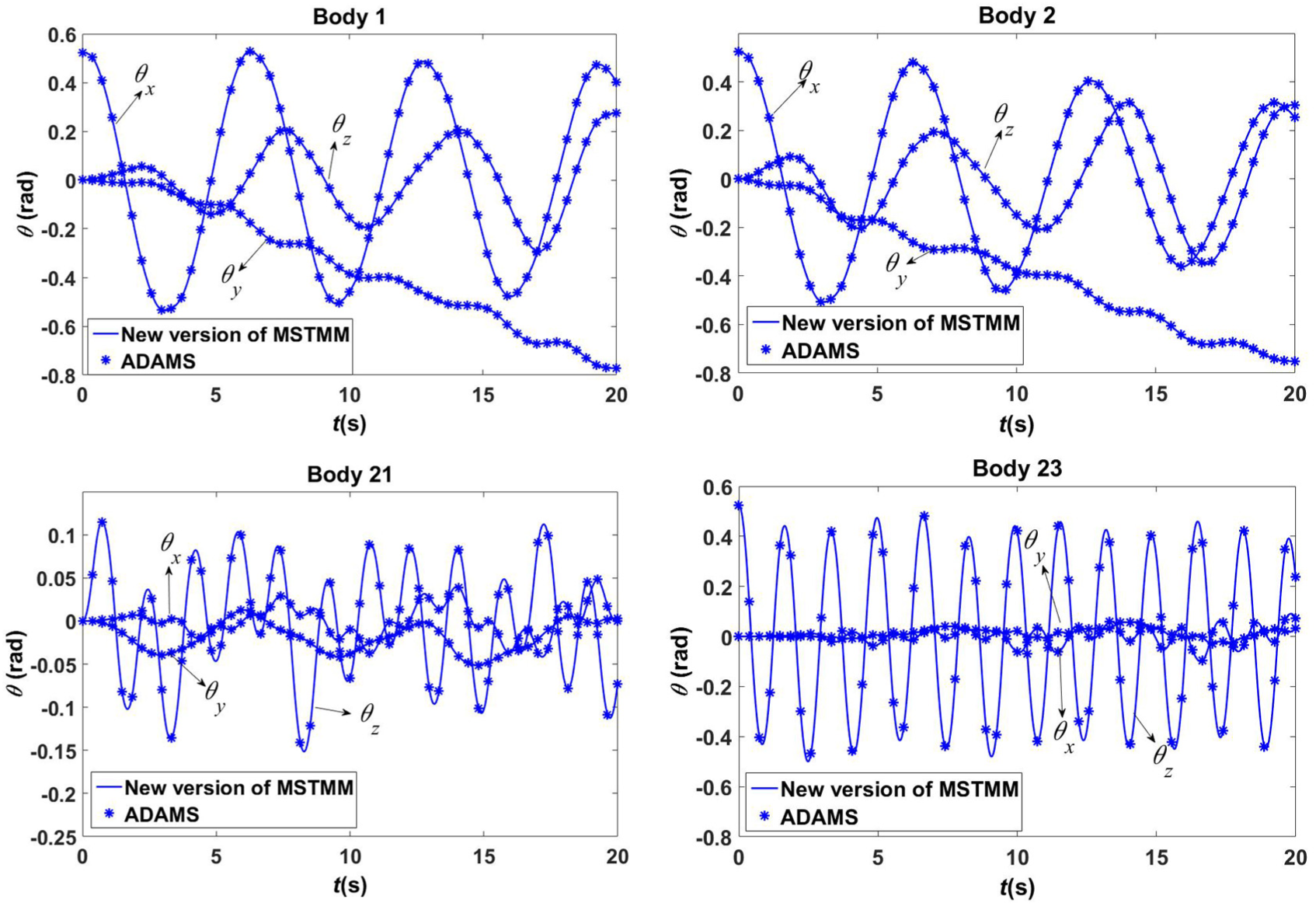
Any tree multibody system may be treated as the assembling of branch subsystems and simple chain subsystems. For instance, in the tree multibody system shown in Figure 4, there are three branch subsystems totally with dotted lines, which are numbered as 24, 25, and 26, respectively. Topology graph of the tree multibody system.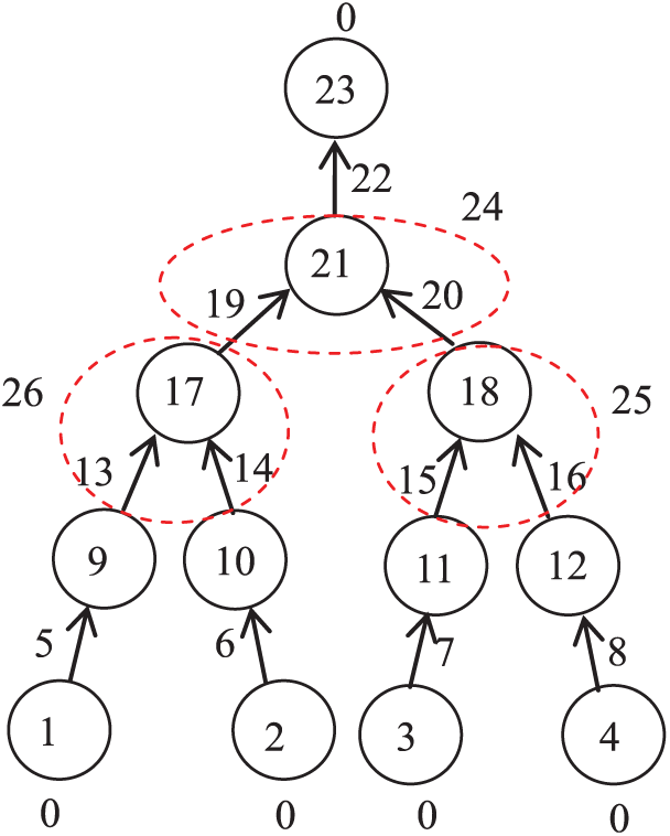

where

For the rest chain subsystems, the following transfer relationships exist

Substitution of equation (66) into equation (68) results in the main transfer equation of system

For each of them with two inputs, there are three geometric equations, which are

Substitution of equation (66) in equation (70) results in

Substituting equation (68) into equation (71), the geometric equations may be expressed by the boundary sate vectors
where
According to equation (9), the overall state vector of system boundaries in Figure 4 is

The overall transfer equation of system is consistent with equation (10).
Substituting the main transfer equation (69) and geometric equation (72) into equation (10), the overall transfer matrix may be obtained

where
Overall transfer equation for closed-loop-and-branch-mixed systems
Closed-loop subsystem transform
For the closed-loop subsystem composed of bodies 1, 2, 5, 6, 9 and hinges 3, 4, 7, 8, 11 as shown in Figure 5, the loop is “cut off” at point

where


(a) Closed-loop subsystem and (b) branch system after cutting off the closed loop.
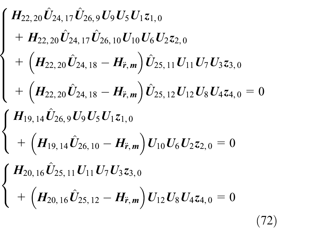
The overall transfer equation for closed-loop-and-branch-mixed systems
For the closed-loop-and-branch-mixed system in Figure 2, after “cutting off” the closed loop at point

Topology graph of a closed-loop-and-branch-mixed system after cutting off closed loop.
Along the transfer path, the main transfer equation is
and geometric equations for three branch subsystems are

where

as well as the supplement equation for closed loop is

The overall state vector of system boundaries is

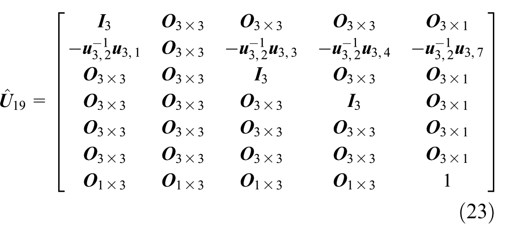
Substituting the main equation (78), geometric equation (79), and the supplement equation (81) into equation (10), the overall transfer matrix is

where

Matrix
Automatic deduction theorem of overall transfer equation for tree systems as well as closed-loop-and-branch-mixed systems
Considering equations (10), (73)–(75) and equations (82)–(84) comprehensively, following features of the new version of MSTMM may be summarized, which forms automatic deduction theorem of overall transfer equation for tree systems as well as closed-loop-and-branch-mixed systems.
Tree systems
The overall transfer equation for tree multibody system is composed of two parts: the main transfer equation and geometric equations:
The first row of the overall transfer matrix corresponds to the main transfer equation, where the coefficient matrix of root state vector is minus identity matrix. The coefficient matrices of tip state vectors (such as
The quantity of geometric equations is the sum of non-first inputs of all branch subsystems in the tree multibody system. The structure of coefficient matrices corresponding to tip state vectors obeys: the coefficient matrix from one tip till the output of a branch subsystem, via the first input hinge of the branch subsystem (such as
Closed-loop-and-branch-mixed system
The overall transfer equation for closed-loop-and-branch-mixed systems is composed of three parts: the main transfer equation, geometric equations, and supplement equations. The statements of coefficient matrices in the main transfer equation and geometric equations are similar as those for tree systems.
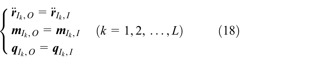
As for the supplement equations, the quantity of supplement equations is equal to the number of closed-loop subsystems. After a closed-loop subsystem is “cut off,” a pair of “new boundaries” will be generated at the “cutting-off” point, of which the state vectors are equivalent in theory, however, transmitted in opposite directions. Therefore, according to label convention, the accelerations and angular accelerations are equal, while the internal forces and internal moments are opposite equal. Consequently, the relationship of the pair of “new state vectors” may be described by a supplement equation (such as equation (54)), that is, one state vector is equal to Matrix
Numerical examples
Tree MSD
In Figure 4, body 23 is hang on ceiling by a smooth ball-and-socket hinge, that is, the boundary at body 23 is simply supported. Boundaries at bodies 1, 2, 3, and 4 are free. System boundary conditions are given as

and the initial conditions are
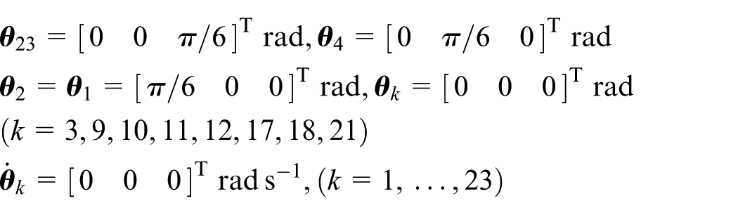
All hinges are smooth ball-and-socket hinges, and structure parameters of all rigid bodies are listed in Table 1, where m is the mass of rigid body,
Structure parameters of rigid bodies.
where

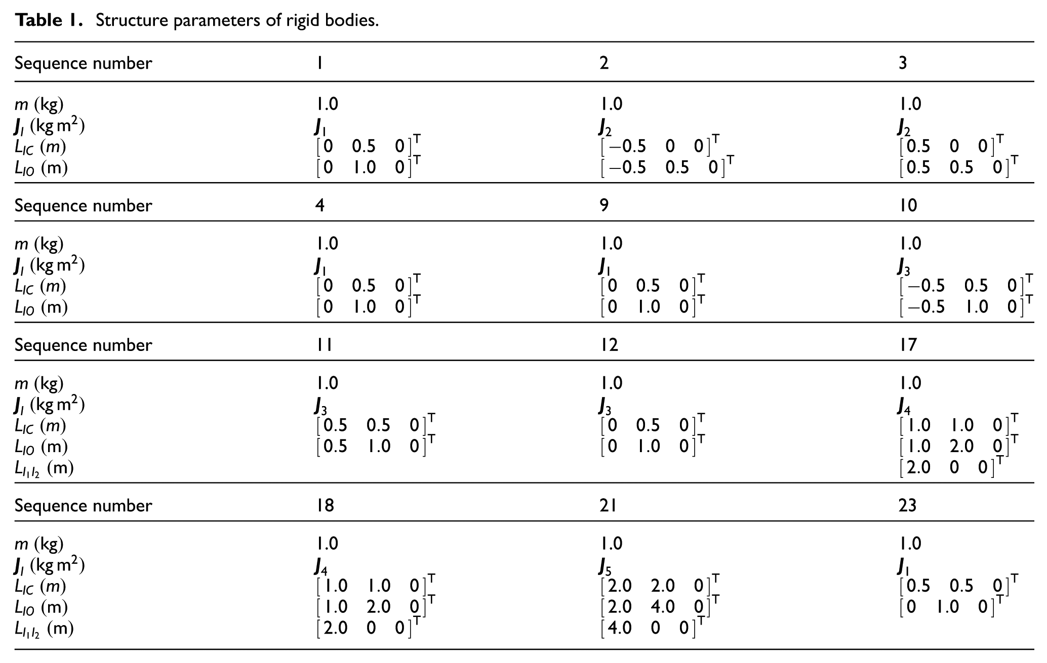
The tree MSD are computed by the new version of MSTMM and ADAMS software, respectively. Time history of rotation angles in three orientations of four rigid bodies are shown in Figure 7. It can be seen that the results obtained by these two methods have good agreements, which validates the automatic deduction method of overall transfer equation for tree multibody systems.
Time history of rotation angles of body 1, 2, 21, and 23 in tree system.
Dynamics of closed-loop-and-branch-mixed systems
In the closed-loop-and-branch-mixed system shown in Figure 2, body 23 is hang on ceiling by a smooth ball-and-socket hinge. A pair of “new boundaries” are generated after “cutting off” the closed loop at point

and the initial conditions of the system are

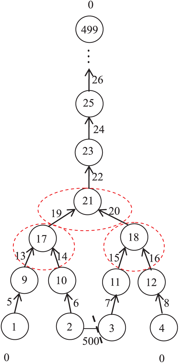
Hinge 24 is a smooth ball-and-socket hinge, while the structure parameters of all the other elements are identical to the corresponding elements in the example of tree multibody system. The dynamics of the mixed system are computed by the new version of MSTMM and ADAMS software. The computational results are given in Figure 8, from which results by these two methods are in good agreements. This validates the automatic deduction method of overall transfer equation for closed-loop-and-branch-mixed systems.

Time history of rotation angles of body 1, 2, 21, and 23 in mixed system.
Dynamics of large closed-loop-and-branch-mixed systems
The large closed-loop-and-branch-mixed system containing 250 rigid bodies is shown in Figure 9. Body 499 is hang on ceiling by a smooth ball-and-socket hinge. Boundaries of body 1 and body 4 are free. The closed loop is “cut off” at point

The system initial conditions are

All hinges are smooth ball-and-socket hinges, and the structure parameters of body 1, 2, 3, 4, 9, 10, 11, 12, 17, 18, 21, and 23 are the same with that of the same sequence number in Table 1. The structure parameters of body 25, 27, 29,…, 499 are the same with those of body 23.
Topology graph of the large mixed system with 250 bodies.
The dynamics of large closed-loop-and-branch-mixed system are computed by new version of MSTMM with Riccati transformation10,11 and ADAMS software. The rotation angles varied with time of four rigid bodies are depicted in Figure 10, from which the results obtained by these two methods have good agreements.
Time history of rotation angles of body 1, 2, 18, and 21 in large mixed system.
The overall transfer matrix of chain system is equal to the successive multiplication of transfer matrices of all elements. Due to the constant order of transfer matrix (the order of transfer matrix is 7 with planar motion while 13 with spatial motion), the system works with
Computational complexity of dynamical methods.

Conclusion
By defining branch subsystems, the general transfer equation and transfer matrix for branch subsystems are developed, which simplifies the deduction process and form of overall transfer equation of system greatly for complicated multibody systems.
Accordingly, the tree multibody system may be regarded as the assembling of branch subsystems and simple chain subsystems. Thus, it is convenient to establish the overall transfer equation and to realize programming using the automatic deduction of overall transfer equation for tree multibody systems.
Meanwhile, by “cutting off” the closed-loop subsystem, any closed-loop-and-branch-mixed system may be treated as a tree multibody system with “new boundaries,” further, as the assembling of branch subsystems and simple chain subsystems. It becomes convenient to establish overall transfer equation for closed-loop-and-branch-mixed system, and automatic deduction of overall transfer equation for closed-loop-and-branch-mixed system is realized.
In comparison of the proposed method and ADAMS software, the results show that the proposed method is valid and has following features: no need of global dynamics equation; high computational speed, such as, for the third numerical example, it takes 6.52 s by the proposed method to compute the system dynamics, while 238 s by ADAMS; highly programmable and convenient to be applied in engineering.
In comparison of the new version of MSTMM to recursive method by Brandl et al. 9 , the new version of MSTMM through Riccati transformation is a little more efficient than the nth order recursive method.
In general, any multibody system, according to its topology graph, may always be categorized into one of the following systems: chain systems, closed-loop systems, branch systems, tree systems, or closed-loop-and-branch-mixed systems. Automatic deduction theorem of overall transfer equation has been given for chain systems and closed-loop systems of new version of MSTMM in Rui et al. 19 and for branch systems of new version of MSTMM has been given in Rui et al. 20 Hence, automatic deduction theorems of overall transfer equation for general systems are composed by and Rui et al.19,20, and this paper together.
Footnotes
Appendix 1
Acknowledgements
The authors owe special thanks to Prof. Dieter Bestle from Brandenburgische Technische Universität, for his instructive suggestions and offering lots of important discussion on this article during his visit to Institute of Launch Dynamics, Nanjing University of Science and Technology.
Handling Editor: Crinela Pislaru
Declaration of conflicting interests
The author(s) declared no potential conflicts of interest with respect to the research, authorship, and/or publication of this article.
Funding
The author(s) disclosed receipt of the following financial support for the research, authorship, and/or publication of this article: The research in this article is supported by Research Fund for the Doctoral Program of Higher Education of China (20113219110025, no. 20133219110037), Nature Science Foundation of China Government (11472135), and Program for New Century Excellent Talents (NCET-10-0075).