
Abstract
Although reinforced concrete shear wall structures are widely used in high-rise buildings, the methods used to analyze the seismic response of such a structure during an earthquake generally have low calculation efficiencies. In this article, the transfer matrix method of multibody systems is first established as a mechanical model of a regular reinforced concrete shear wall structure with both bifurcated and closed transfer paths to analyze the seismic responses of structures. By separating the shear wall legs, establishing a state vector relationship between the two endpoints of the coupling beams, and combining all state vectors of the inputs or outputs of each shear wall leg, the total transfer between shear wall legs is realized, and the overall transfer equation and overall transfer matrix of a shear wall structure are obtained. Applying the transfer matrix method of multibody systems, a 15-story shear wall structure is used as an engineering example to analyze seismic responses for frequent and rare earthquakes using MATLAB software. The findings show that the transfer matrix method of multibody systems provides similar results to ANSYS but that the transfer matrix method of multibody systems greatly increases calculation efficiency while maintaining accuracy.
Keywords
Introduction
Urban population density has been increasing with the development of high-rise buildings, and the consequences of earthquake damage on these buildings are severe. In 2010, an M8.8 earthquake in Chile caused serious damage to high-rise buildings; as a result, 486 people died and 79 went missing. Among all earthquakes that have occurred in recent years, this earthquake caused the most severe damage to high-rise buildings and it drew the wide attention of researchers both at home and abroad. 1 Because China is located at the junction of two earthquake belts, seismic activity is frequent. In 2008, an M8.0 earthquake in Wenchuan in Sichuan Province 2 caused different degrees of damage to high-rise buildings in Chengdu and other cities. The main focus of seismic research on high-rise structures is determining how to establish reasonable mechanical models for different structures, and how to use efficient calculation methods for dynamic analyses of these structures. In this structure dynamic analysis method, the total mass matrix, stiffness matrix, and damping matrix of a structure must be determined to establish the general dynamic equation, and they must be derived again if the model elements change. Because the order of the matrix in the equation is usually equal to the total degrees of freedom, the dynamic analysis workload for a high-rise structure is heavy, and the process is complex. In addition, with the continuous development of structural vibration control,3,4 the traditional dynamic calculation method cannot meet the vibration control requirements because of its low computational efficiency. Therefore, developing an effective and rapid calculation method is important in terms of both theoretical significance and engineering application value.
The seismic analysis methods for a shear wall structure primarily include response-spectrum, push-over, and time-history analysis methods. The response-spectrum method cannot be used for elastic–plastic time-history analysis; thus, it cannot accurately analyze the plastic state of a structure. The push-over analysis method is actually a static nonlinear analysis method that can simplify the design work, but the results deviate substantially from the observational data. The time-history analysis method considers the peak ground motion, ground motion duration, and frequency spectrum characteristics, among other factors, and it can accurately describe the whole process of structure response under seismic action and determine the internal forces and displacements in each moment. At present, the dynamic time-history analysis of a high-rise structure is achieved primarily using finite element software, such as ABAQUS, ANSYS, and MIDAS.5–7 Although the application of finite element software in high-rise structures is increasing, problems such as its complex calculation model, time-consuming nature, and lack of convergence in elastic–plastic analysis must be solved. The transfer matrix method of multibody systems (MSTMM) was first proposed by Professor Xiaoting Rui and his academic team in 1993; after decades of practical engineering application and constant improvement, it has been developed into a new highly stylized and efficient method of describing multibody system dynamics. In recent years, it has been used in the fields of weaponry, vehicles, aerospace, and aviation, among others. For instance, Rong et al. 8 used the discrete time MSTMM for the dynamic analysis of the coupling of the self-propelled artillery system, derived the transfer matrix of the typical elements in complex spacecraft and the transfer equation, and developed a highly efficient dynamic modeling method to realize the fast calculation of spacecraft dynamics. 9 Due to the importance of the ballistic trajectory computation, including the estimation of the launch point and impact point problems, a fast and accurate model is needed to increase the weapon precession. Khalil et al. 10 used a discrete time transfer matrix method (TMM) to compute the trajectory of both fin- and spin-stabilized artillery projectiles. The feasibility of using the TMM to analyze open variable-thickness circular cylindrical shells exposed to a high-temperature field was explored theoretically. In the utilized approach to the problem, the thermal degradation of the thermoelastic characteristics of the material is considered. Abbas et al. 11 investigated in detail the natural frequencies and mode shapes of the cylindrical shells by combining the vibration theory with the MSTMM. For the rigid flexible system of bifurcated and closed loops, Zhao et al. 12 used the MSTMM to establish a mechanical model of a multi-layer leather cutting bed rotor body and compared the results obtained using the dynamic analysis and those obtained using the finite software ANSYS. MSTMM contains a consistent view on the classical TMM, extends to multibody systems with general topology, and applies to some important engineering problems. The advantages of the MSTMM include the following: this method does not need the global dynamics equations of the system, usually obtains a low order of the system matrix, has high computational efficiency, and avoids the “morbidity” problems inherent to eigenvalue calculations. The MSTMM has also been applied in the field of civil engineering. Sun and Li 13 derived a precise transfer matrix format for buckling analysis of a compression bar under an axial load and calculated the critical loads of the compression bar with different boundary constraints based on the theory of the precise transfer matrix method. They derived the transfer matrixes from the planes of curved bridges based on the fast Fourier transform (FFT) and determined the relationship between the quality and the inertial force of the point transfer matrix for vibration analysis. 14 They also combined the TMM and the computing skills of exponent for precise integration method and dynamically analyzed the structure in the frequency domain. 15
In this article, based on the mechanical model for a shear wall structure, the MSTMM is used to calculate and analyze the elastic response of a shear wall structure during frequently occurring earthquakes and its elastic–plastic responses during rarely occurring earthquakes. The findings are then compared to the results obtained by the traditional ANSYS method. The calculation efficiencies of these two methods are also compared.
Mechanical model of a regular reinforced concrete shear wall structure and its transfer matrix
Mechanical model of a reinforced concrete shear wall element
Based on the MSTMM, the reinforced concrete (RC) shear wall structure is decomposed into the shear wall element and the coupling beam element. The improved multiple-vertical-rod element model is chosen as the mechanical analysis model of the shear wall element. 16 As shown in Figure 1, the axial and shear springs of the vertical rod represent the axial and shear stiffnesses of the shear wall body subunits, respectively, and the upper and lower rigid bodies connected with the vertical rod represent the upper and lower floor subunits, respectively. This model not only retains the advantages of the multiple-vertical-rod element model but also considers the interaction of the shear and axial stiffnesses of the shear wall, better representing the actual situation.

Mechanical model of an RC shear wall element.
The mechanical model of an RC shear wall body subunit is shown in Figure 2. Here, r = 0.5, (x, y) represents the inertial coordinate system of the shear wall body subunit model. If the upper and lower midpoints of a shear wall body subunit are assumed as the output O and the input I, respectively, the shear wall body subunit is divided into multiple vertical rods numbered 1, 2,…, n.
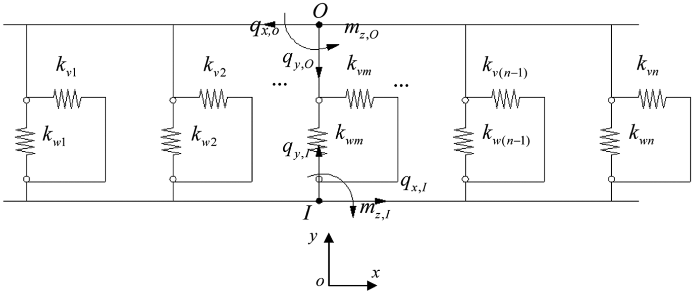
Mechanical model of an RC shear wall body subunit.
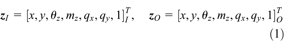
We define the state vectors of the input and output of a shear wall body subunit as follows
Taking the shear spring of vertical rod m as the analysis object, the horizontal coordinates of endpoint O can be expressed by the geometric relationship as

The horizontal coordinates of endpoint I can be expressed as

After linearizing the trigonometric function in equations (2) and (3), the relative displacement of the shear spring is

According to the force relationship of the shear spring, we have

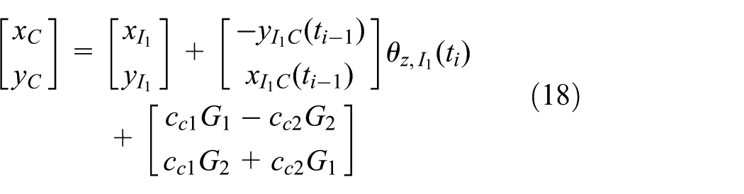
Similarly, the vertical coordinate of endpoint O of the axial spring in vertical rod m can be expressed as

The vertical coordinate of endpoint I can be expressed as

After linearizing the trigonometric function in equations (6) and (7), the relative displacement of the axial spring is

where h represents the height of a shear wall body in this layer.
According to the force relationship of the axial spring, we have

The relationship between the forces of the springs and both the input and output ends can be expressed as

Incorporating equations (5) and (9) into equation (10), we have

where


According to the force equilibrium relationship between the input and output of a shear wall body, we can obtain

According to equations (11) and (12), we can obtain the transfer equation of a shear wall body subunit

where the extended transfer matrix is


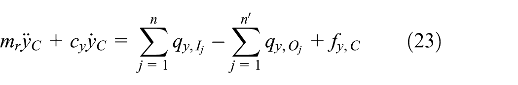
Because a floor subunit is represented by a rigid body with multi-input and multi-output, this study primarily derives the transfer matrix and transfer equation of a rigid body with multi-input and multi-output, as shown in Figure 3. Here, (x, y) represents the inertial coordinate system of the multi-input and multi-output rigid body model, where (x1, y1) is fixed in the first input, and the coordinate system (x2, y2) is obtained by rotating (x1, y1).

Mechanical model of multi-input and multi-output rigid bodies.
According to the geometric relationship of the rigid body motion and using the linearized trigonometric function, we have


where
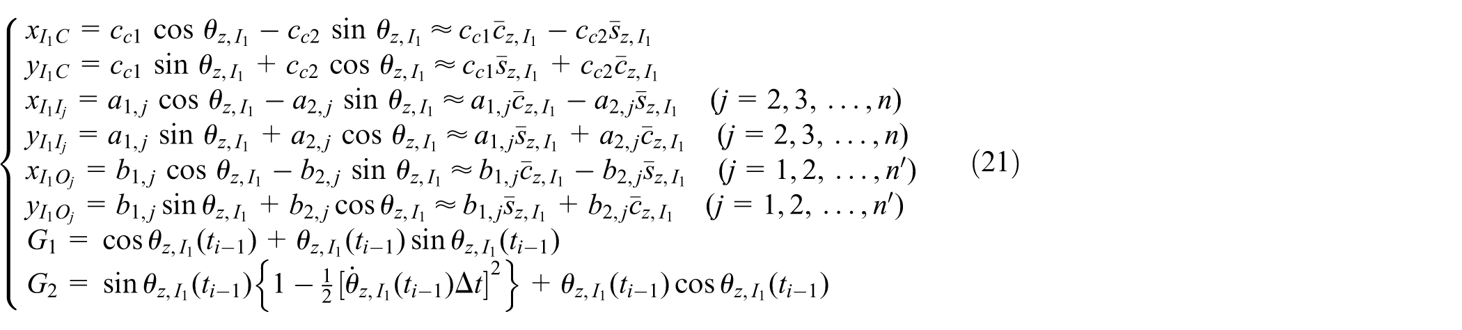
Here,
The external force
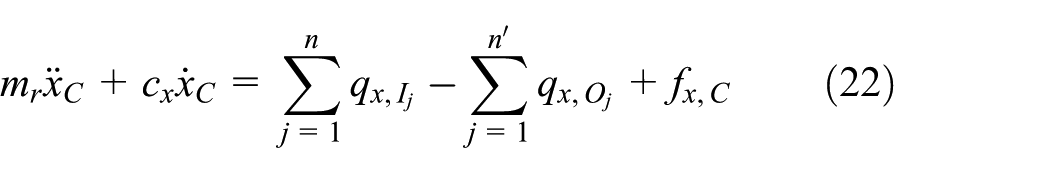
where
Based on the absolute angular momentum theorem, we have

Linearizing equations (22)–(24), we have


Rewriting equations (16) and (19) in matrix form, we have

where

Rewriting equations (17) and (20) in matrix form, we have

where

Rewriting equations (25)–(27) in matrix form, we have

where


We define the state vectors as follows

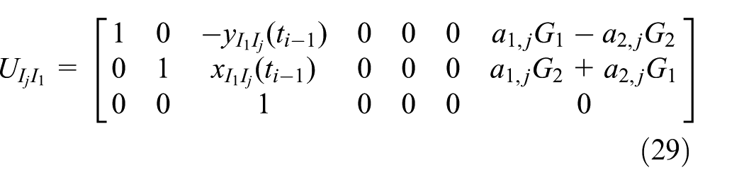
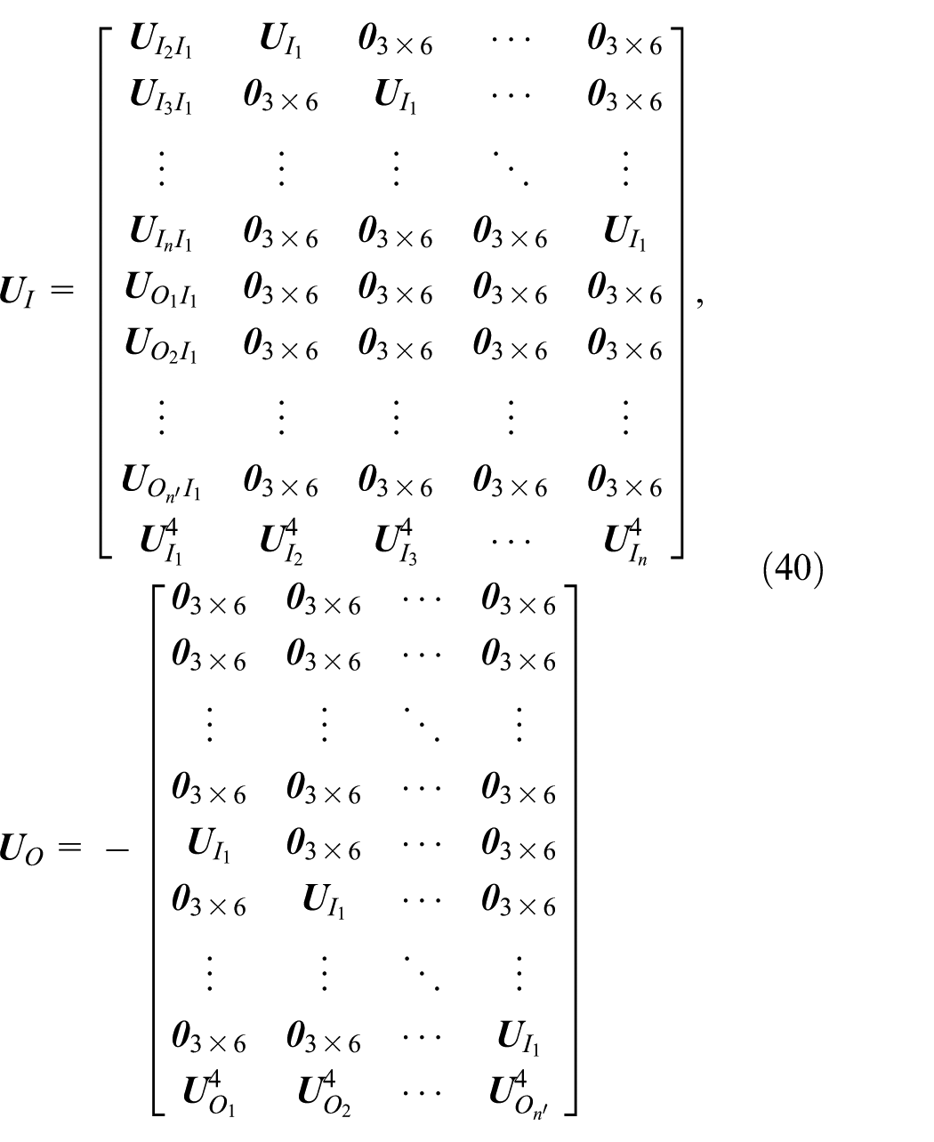
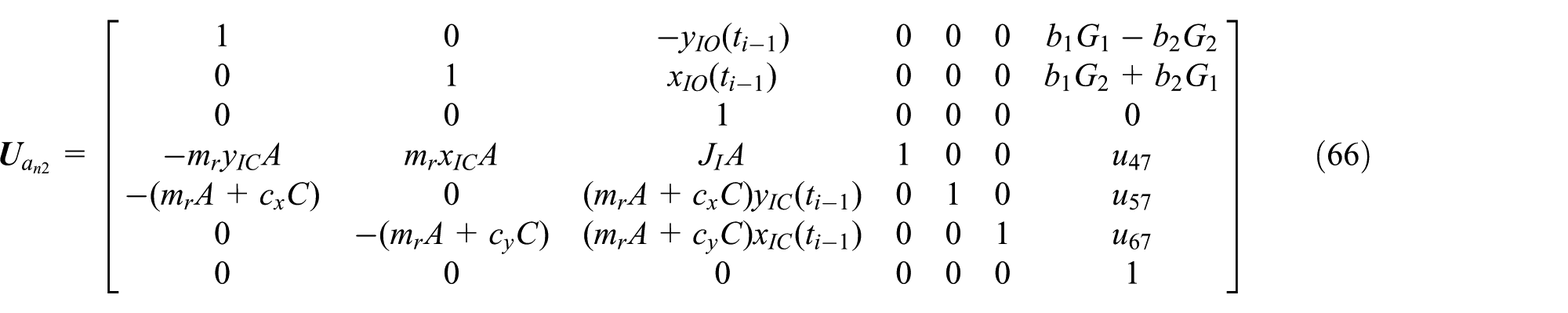
Combining equations (28), (31), and (33), we can obtain the transfer equation of the floor subunit as a rigid body with multi-input and multi-output as follows

where the transfer matrixes are
Mechanical model of a coupling beam element
Because the stiffness of the part extending into the shear wall in a coupling beam can be regarded as infinite, 17 the connection between the beam and the wall can be simplified into a local rigid domain. To reflect the forces of the endpoint in a coupling beam, we use a composite spring to simulate the domain, with the axial, shear, and bending springs representing the axial, shear, and bending stiffnesses, respectively. Assuming no external force on the mid-span in a coupling beam, 18 the middle part can be regarded as a massless elastic beam. The mechanical model of the coupling beam element is shown in Figure 4. Here, (x, y) represents the inertial coordinate system of the coupling beam element model. The rigid domains are 1 and 5, the composite springs are 2 and 4, and the massless elastic beam is 3.

Mechanical model of a coupling beam element.
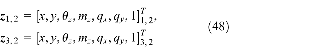
We take the left rigid domain 1 in the mechanical model of coupling beam and define the state vectors of the input and the output, which are, respectively

Under the inertial coordinate system, we have the following geometric relationship
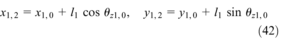

Linearizing equation (42), we can obtain
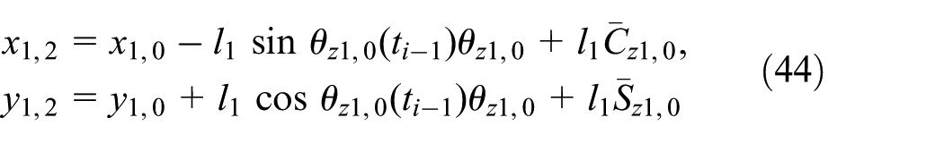
According to the force relationship, we have

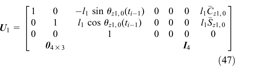
Rewriting equations (43) and (45) in matrix form, we can obtain the transfer equation of rigid domain 1 as follows

where the extended transfer matrix is
Define the state vectors of the input and the output of composite spring 2 as, respectively
The transfer equation is

where the extended transfer matrix of composite springs is

where
Mechanical model of a massless elastic beam 3 is shown in Figure 5. We define the state vectors of the input and the output as, respectively


Mechanical model of a massless elastic beam.
Based on mechanics and the geometric relationship, we can obtain the position coordinates of the output in direction y under the inertial coordinate system as follows

Linearizing equation (52), we have

Based on the relationship between force and position, we can obtain

Rewriting equation (54) in matrix form, we can obtain the transfer equation

where the extended transfer matrix of the elastic beam is

The derivation of the transfer matrix of right domain 5 in the coupling beam is the same as that for the left domain 1. The derivation of the transfer matrix of right composite spring 4 is the same as that for composite spring 2. The total transfer equation of the coupling beam element can be expressed as

where the total extended transfer matrix is

Total transfer equation of shear wall structure
Because the stiffness of a shear wall is large in the plane of the wall and small outside of the plane, the regular spatial structure of the shear wall arrangement can be simplified into a planar structure. The total mechanical model of the shear wall structure is formed by the mechanical model of the shear wall elements and the coupling beam elements. In this research, we chose a three-wall leg shear wall structure as the analysis object. The calculation model is shown in Figure 6. For a general n-wall leg shear wall structure, the derivation procedure of each middle wall leg is similar to that of wall leg b in Figure 6, so the calculation model has universal significance.

Calculation model of the RC shear wall structure.
The three pieces of the wall leg are labeled a, b, and c. The bottom endpoints are labeled a0, b0, and c0. The transfer of each layer in the wall legs a and c involves three parts—the shear wall body subunit, the floor subunit as a rigid body, and the rigid domain in the coupling beam, which are numbered 1–3, respectively. Therefore, the three transfer elements of the
For wall leg a, the transfer begins with a0. According to the transfer equation of the shear wall element, we have

where
The floor subunit as a rigid body

where the transfer matrix of a floor with one input and two outputs as a rigid body is

Separating the state vectors of the two outputs, we can obtain

where
Inserting equation (59) into equation (62), we can obtain the transfer equation

In the same way, we can obtain

The top floor as rigid body

where the transfer matrix of the top floor with one input and one output is
Because there are a tremendous number of elements and bifurcated and closed-loop transfer characteristics in the mechanical model of the shear wall structure, establishing the overall transfer equation using the general MSTMM will lead to many problems, including multi-inputs and multi-outputs in the transfer of the structure, a complex transfer path, and a boundary relationship that is difficult to describe. To overcome these problems, wall legs a and b in the shear wall structure must be separated using the free-body technique. The overall transfer between shear wall legs a and b is accomplished using the relationship of state vectors on the forces and displacements between the left and right endpoints of coupling beams
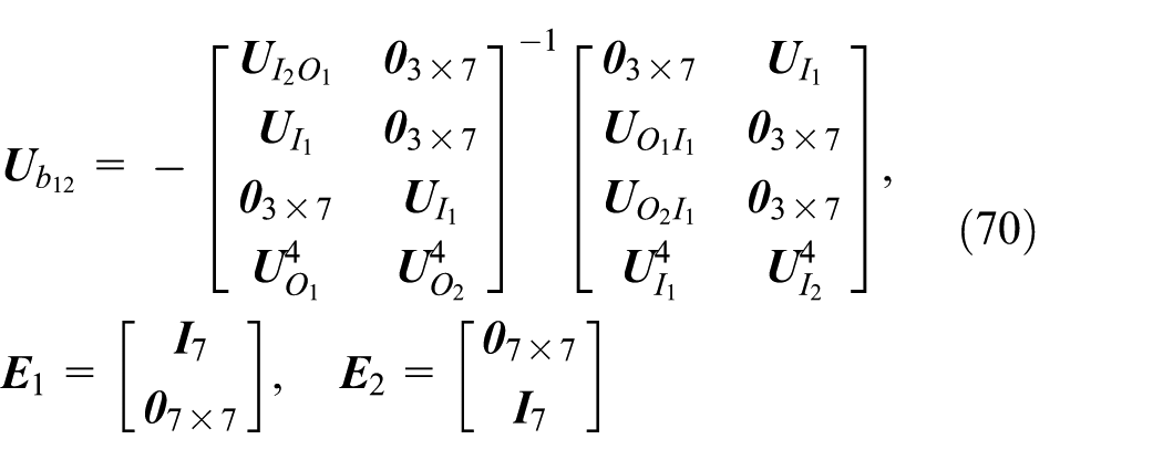
Therefore, we can obtain the relationship between the right state vectors in the coupling beams and

where

For wall leg b, the transfer begins with b0. The floor subunit as rigid body

where
Separating the state vectors of the two outputs by applying


Rewriting equations (71) and (72) in matrix form

We define

We assume
Using the same method as that used for the overall transfer between shear wall legs a and b, the transfer relationship between shear wall legs b and c can be obtained as follows

where we define

For wall leg c, the transfer begins with c0. Floor

where the transfer matrix

Based on the transfer relationship, we can obtain

For the top floor

where

Based on the transfer relationship, the transfer equation of the top floor as rigid body

From equation (82), we have

where we define
In addition, for top floor

From equation (85), we have

where we define

According to the boundary condition of top floor

where

Combining equations (67), (73), (75), (83), and (86), we can obtain


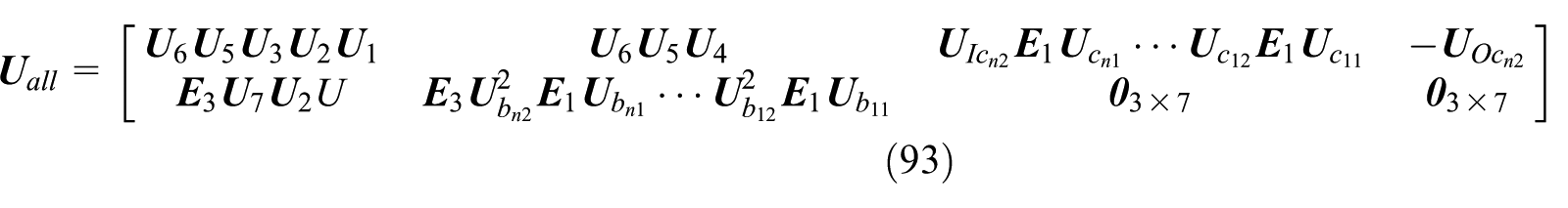
Combining equations (90) and (91), we can obtain the total transfer equation of the overall shear wall structure as follows

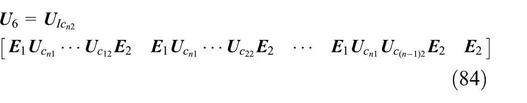
where the total transfer matrix of the shear wall structure is shown as follows
Calculation process
Calculation process for the eigenperiods of a shear wall structure
According to equation (92), solving the eigenperiods and seismic response of a structure is based on the system’s boundary state vectors. Because the displacements, angular displacements in

In order to get the nonzero solution of equation (94), we have

The calculation process for the eigenperiods of a shear wall structure is shown in Figure 7.

Calculation process for eigenperiods of a shear wall structure.
Calculation process for the responses of a shear wall structure during earthquakes
During a frequently occurring earthquake, the structure is in the elastic state, at which the stiffness remains constant. During a rarely occurring earthquake, the structure enters into the elastic–plastic stage, at which the stiffness depends on the restoring force model and its changes are assessed by the calculated displacement and speed at a given time. Based on the MSTMM, the calculation of the response of a shear wall structure during earthquakes is performed using MATLAB software. The calculation process for the responses of a shear wall structure during earthquakes is shown in Figure 8.

Calculation process for responses of a shear wall structure during earthquakes.
Stiffness of the elements in a shear wall structure
Because the elastic–plastic response of a shear wall structure happens during a rarely occurring earthquake, we must choose the restoring models or stiffness skeleton curves for all elements in the structure.
The bilinear restoring model 19 is used to acquire the axial stiffness of vertical rods in shear wall body subunits, as shown in Figure 9.

Restoring force model for the axial stiffness of a vertical rod in shear wall body subunits.
When a vertical rod in shear wall body subunits is under tension, the parameters can be expressed as follows

where
When the vertical rod in the shear wall body subunits is under pressure, assuming the reinforcement and concrete yield simultaneously, the parameters are shown as follows

where
To simulate the shear model for the vertical rod of shear wall body subunits, the nonlinear shear mechanism hypotheses proposed by AA Hashish 20 are chosen. From different states of the vertical rods under tension or compression, the shear stiffness can be obtained as follows
1. The elastic state under compression is

2. The elastic state under tension is
3. The yielding state under pressure is

4. The yielding state of tensioned steel is

5. The unloaded state after tensile yield is

6. The unloaded state after compressive yield is

In these equations,

Stiffness skeleton curves for the endpoint composite springs in a coupling beam element.
The parameters for the stiffness skeleton curves of the axial spring in a coupling beam element are as follows
where r represents the ratio of reinforcement;
The parameters for the stiffness skeleton curves of the shear spring in a coupling beam element are as follows

where k is a friction coefficient, and its value is 0.33; b and h are the width and height of the coupling beam section, respectively;
The parameters for the stiffness skeleton curves of bending spring in a coupling beam element are as follows

where
Engineering example
Structural parameters
A typical 15-layer shear wall structure is chosen as an example, as shown in Figure 11. The layer height is 2.9 m, the seismic fortification intensity is set to 7, the site type is II, and the designed earthquake is designated as being of the first classification. The strength grade of the concrete used in the columns is C30, the reinforcement is grade HRB400, and the coupling beam section size is 200 mm × 500 mm. The details are shown in Figure 11(b) and (c).

Diagram of the shear wall structure and its details: (a) diagram of the shear wall structure, (b) details of flange and web, and (c) details of coupling beams k and l.
Because the mass and the lateral stiffness distributions in the regular shear wall structure are basically averaged over the longitudinal direction, the lateral earthquake action undertaken by each plane shear wall structure is nearly equivalent. Thus, the original spatial structure can be simplified as a planar structure under the lateral action of an earthquake. In this article, the plane shear wall structure in axis ② is chosen as a plane analytical model in the shear wall structure.When analyzing the responses of the shear wall structure during earthquakes, we use the following parameters: elastic modulus E = 3.12 × 10¹⁰ N/m2; the number of vertical rods in shear wall element n = 14; kv and kw of each vertical rod are the same and their values are computed by the related formulas in the section “Stiffness of the elements in a shear wall structure”; the masses of rigid bodies
To analyze the results obtained by the MSTMM, the finite element software ANSYS was used to calculate the shear wall structure for comparison. Because the structure is regular, BEAM188 was selected as the model for both the beam and shear wall elements, and SHELL63 was selected as the model for the floor elements, as shown in Figure 12. The material properties are as follows: modulus of elasticity = 3.12 × 10¹⁰ N/m2, Poisson’s ratio = 0.2, mass density = 2500 kg/m3, and damping ratio = 0.05.
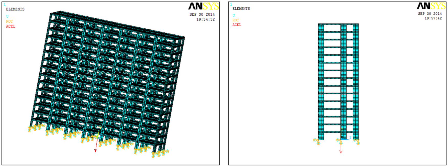
Analyzed ANSYS model of the shear wall structure.
Analysis on the eigenperiods of the shear wall structure
According to Figure 7, based on the MSTMM and ANSYS, the eigenperiods of the structure are shown in Table 1.
Eigenperiods calculated by two different methods.
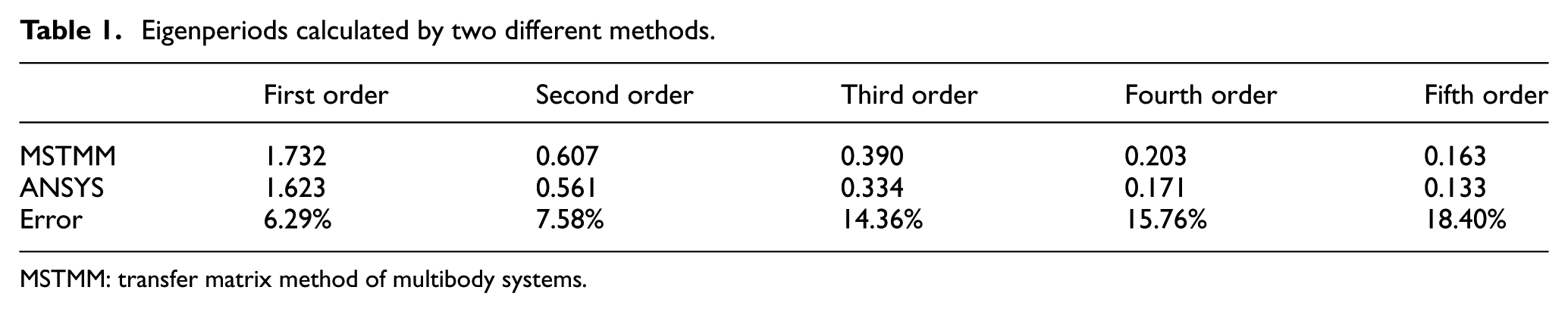
MSTMM: transfer matrix method of multibody systems.
As observed in Table 1, the error of the first-order period obtained by MSTMM and ANSYS is 6.29%, and with the increase in order, the error is also increasing. The eigenperiods calculated by ANSYS are all smaller than those by MSTMM, because of the interaction in space model established by ANSYS and the large matrix numbers of MSTMM. The calculation time by MSTMM was approximately 1/28th of that by ANSYS. The high calculation efficiency of MSTMM is obvious.
Analysis of the seismic response of the shear wall structure during frequently occurring earthquakes
Because the seismic fortification intensity is 7 (the designed earthquake is designated as being of the first classification), according to the seismic code of the PRC (GB 50011-2010), 22 the peak value of the acceleration versus the time data should be less than 35 cm/s2 when studying the responses of structures under frequently occurring earthquakes. In this study, two natural earthquake waves (the El Centro and Taft earthquake waves) and one artificial earthquake wave (the Nanjing earthquake wave) are chosen. The duration time is set 10 s to focus on the dynamic time-history analysis for the top displacement of the shear wall structure and the base shear force of shear wall leg b using both the discrete time MSTMM and the finite software ANSYS.
Based on the MSTMM and ANSYS, the top displacement time-history curves of the structure during the frequently occurring El Centro, Taft, and Nanjing earthquake waves are shown in Figures 13–15, respectively.

Top displacement time-history curves of the structure during frequently occurring El Centro earthquake wave calculated using two different methods.

Top displacement time-history curves of the structure during frequently occurring Taft earthquake wave calculated using two different methods.

Top displacement time-history curves of the structure during frequently occurring Nanjing earthquake wave calculated using two different methods.
As illustrated in Figures 13–15, using the MSTMM and ANSYS, under the activity of the El Centro wave, the maximum top displacements are 34.49 mm at t = 6.22 s and 35.07 mm at t = 9.88 s. Under the activity of the Taft wave, the maximum top displacements are 33.75 mm at t = 7.66 s and 29.79 mm at t = 9.08 s. Under the activity of the Nanjing wave, the maximum top displacements are 35.43 mm at t = 9.66 s and 30.60 mm at t = 8.66 s. The shapes of the displacement time-history curves based on the two methods are similar.
The maximum top displacements determined under the actions of the three earthquake waves by both MSTMM and ANSYS are shown in Table 2; their errors relative to the ANSYS values are also listed.
Maximum top displacements during frequently occurring earthquakes calculated using two different methods.

MSTMM: transfer matrix method of multibody systems.
As observed in Table 2, the errors of the maximum top displacements obtained using the MSTMM and ANSYS methods under the El Centro, Taft, and Nanjing waves are 1.65%, 13.29%, and 15.78%, respectively, and the error of the average value is 8.60%. Thus, the results are similar. However, the errors can be attributed to be the differences between the mechanical models based on these two methods; specifically, the floor in the mechanical model based on the MSTMM is simplified as a rigid body and is a plane structure, whereas the floor in the model based on ANSYS is considered solid and is a spatial structure. In addition, the error depends on not only the dynamic performance of the structure itself but also the input seismic waves. Generally speaking, MSTMM has an obviously superior calculation efficiency; the calculation time using MSTMM was approximately 1/11th of that using the ANSYS method.
Based on MSTMM and ANSYS, the base shear force time-history curves for the shear wall leg b during frequently occurring earthquakes with the El Centro, Taft, and Nanjing waves are shown in Figures 16–18, respectively.

Base shear force time-history curves for shear wall leg b during frequently occurring El Centro earthquake wave calculated using two different methods.

Base shear force time-history curves for shear wall leg b during frequently occurring Taft earthquake wave calculated using two different methods.
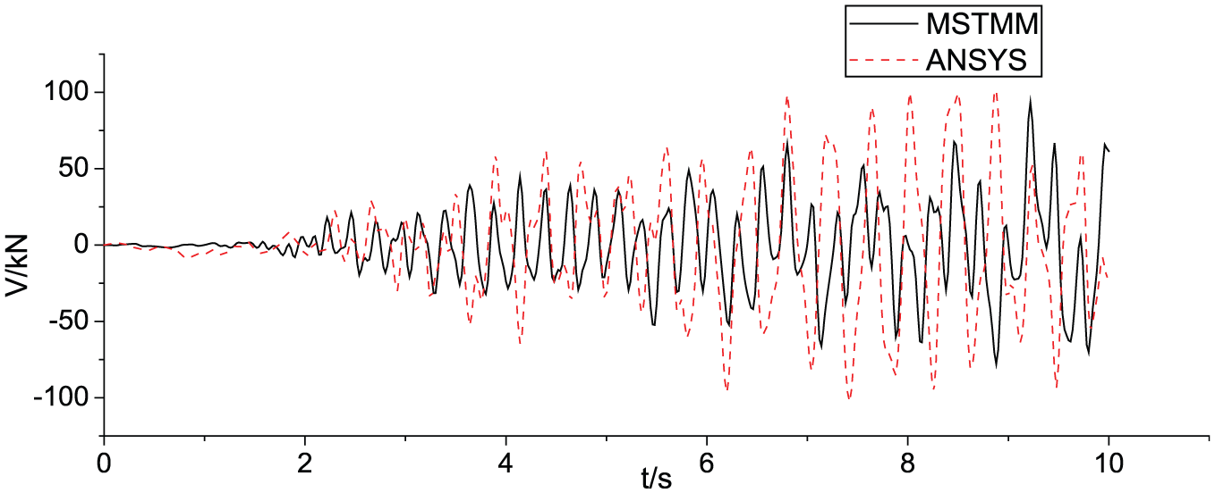
Base shear force time-history curves for shear wall leg b during frequently occurring Nanjing earthquake wave calculated using two different methods.
As illustrated in Figures 16–18, using the MSTMM and ANSYS, under the activity of the El Centro wave, the maximum base shear forces of shear wall leg b are 97.03 kN at t = 6.22 s and 102.47 kN at t = 9.78 s. Under the activity of the Taft wave, the base shear forces of shear wall leg b are 87.67 kN at t = 7.64 s and 99.33 kN at t = 9.52 s. Under the activity of the Nanjing wave, the maximum top displacements are 93.34 kN at t = 9.22 s and 102.55 kN at t = 7.42 s.
The maximum base shear forces determined under the actions of the three earthquake waves by both MSTMM and ANSYS are shown in Table 3; their errors relative to the ANSYS values are also listed.
Maximum base shear forces for shear wall leg b during frequently occurring earthquakes calculated using two methods.
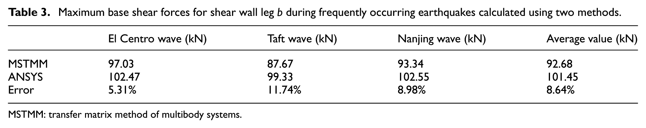
MSTMM: transfer matrix method of multibody systems.
As observed in Table 3, the errors of the maximum base shear forces for the shear wall leg b calculated using the MSTMM and ANSYS methods under the El Centro, Taft, and Nanjing waves are 5.31%, 11.74%, and 8.98%, respectively. Although the results are almost the same, the calculation time using the MSTMM was approximately 1/11th of that using the ANSYS method, reflecting the high calculation efficiency of the MSTMM.
Analysis of seismic response of the shear wall structure during rarely occurring earthquakes
According to the seismic code of the PRC (GB 50011-2010), 22 when the responses of structures under rarely occurring earthquakes are studied, the peak value of the acceleration versus time data should be less than 220 cm/s2. Based on the discrete time MSTMM, the calculation following the process shown in Figure 8 was conducted in MATLAB. Using the finite software ANSYS, the nonlinear problem of structure should be taken into consideration.23,24 This study chose the plastic material option MKIN, which conforms to the actual situation.
Based on the MSTMM and ANSYS, the top displacement time-history curves of the structure during rarely occurring earthquakes under the El Centro, Taft, and Nanjing waves are shown in Figures 19–21, respectively.

Top displacement time-history curves of the structure during rarely occurring El Centro earthquake wave calculated using two different methods.

Top displacement time-history curves of the structure during rarely occurring Taft earthquake wave calculated using two different methods.
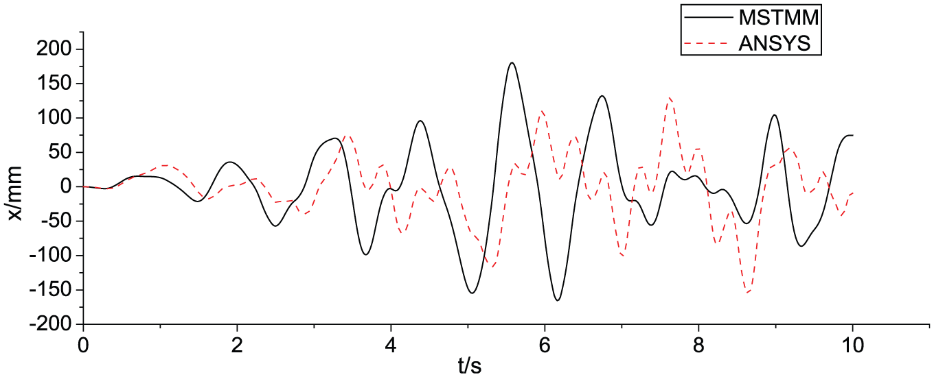
Top displacement time-history curves of the structure during rarely occurring Nanjing earthquake wave calculated using two different methods.
As illustrated in Figures 19–21, using the MSTMM and ANSYS, the maximum top displacements under the activity of the El Centro wave are 158.01 mm at t = 5.52 s and 183.56 mm at t = 8.94 s. Under the activity of the Taft wave, the maximum top displacements are 162.27 mm at t = 7.00 s and 178.54 mm at t = 4.22 s. Under the activity of the Nanjing wave, the maximum top displacements are 180.28 mm at t = 5.58 s and 155.04 mm at t = 8.64 s, respectively. The shapes of the displacement time-history curves based on the two methods are similar.
The maximum top displacements under the actions of the three earthquake waves determined by both the MSTMM and ANSYS are shown in Table 4; their errors relative to the ANSYS values are also listed.
Maximum top displacements during rarely occurring earthquakes calculated using two different methods.

MSTMM: transfer matrix method of multibody systems.
As observed in Table 4, based on the MSTMM and ANSYS, the errors of the maximum top displacements under the El Centro, Taft, and Nanjing waves are 13.92%, 9.11%, and 16.28%, respectively. The error is larger than that during frequently occurring earthquakes. The errors can be attributed to the differences between the mechanical models based on these two methods; specifically, the floor in the mechanical model based on the MSTMM is simplified as a rigid body and is a plane structure, whereas the floor in the model based on ANSYS is considered a solid and is a spatial structure. In addition, the restoring force model of axial and shear springs in the shear wall element and endpoint composite springs in the coupling beam when using the MSTMM is different from that in the plastic model MKIN when using ANSYS. Because the calculation time using the MSTMM was approximately 1/56th of that using the ANSYS method, the MSTMM has an obvious calculation efficiency advantage.
Based on the MSTMM and ANSYS, the base shear force time-history curves for shear wall leg b during rarely occurring earthquakes under the El Centro, Taft, and Nanjing waves are shown in Figures 22–24, respectively.

Base shear force time-history curves for shear wall leg b during rarely occurring El Centro earthquake wave calculated using two different methods.

Base shear force time-history curves for shear wall leg b during rarely occurring Taft earthquake wave calculated using two different methods.

Base shear force time-history curves for shear wall leg b during rarely occurring Nanjing earthquake wave calculated using two different methods.
As illustrated in Figures 22–24, using the MSTMM and ANSYS, the maximum base shear forces for shear wall leg b under the activity of the El Centro wave are 506.93 kN at t = 5.86 s and 578.39 kN at t = 6.16 s. Under the activity of the Taft wave, the base shear forces of shear wall leg b are 533.32 kN at t = 7.62 s and 469.61 kN at t = 7.46 s. Under the activity of the Nanjing wave, the maximum top displacements are 593.11 kN at t = 7.12 s and 569.57 kN at t = 7.44 s.
The maximum base shear forces determined under the actions of the three earthquake waves using both the MSTMM and ANSYS are shown in Table 5; their errors relative to the ANSYS values are also listed.
Maximum base shear forces of the shear wall leg b during rarely occurring earthquakes calculated using two different methods.

MSTMM: transfer matrix method of multibody systems.
As observed in Table 5, based on the MSTMM and ANSYS, the errors of the maximum base shear forces under the El Centro, Taft, and Nanjing waves are 12.35%, 13.57%, and 4.13%, respectively. Although the results are almost the same, the calculation time based on the MSTMM is approximately 1/56th of that using the ANSYS method, reflecting the high calculation efficiency of the MSTMM.
Conclusion
In this article, the MSTMM is first used to establish a mechanical model of an RC shear wall structure. As an engineering example of a shear wall structure, the structure’s seismic responses under the actions of frequently and rarely occurring earthquakes are analyzed. The results of analysis based on the MSTMM are compared to those of analysis based on the ANSYS method, and the following conclusions are drawn:
According to the mechanical model of regular RC shear wall structure established in this article, the transfer matrixes of the shear wall and coupling beam elements are derived. Because there are a large number of elements and characteristics with both bifurcated and closed transfer paths in the model, the total transfer between shear wall legs is realized by separating the shear wall legs, establishing the relationship of state vectors between the two endpoints of coupling beams, and combining all state vectors of the inputs or outputs of each shear wall leg. The overall transfer equation and overall transfer matrix of a shear wall structure are also obtained.
As the engineering example of a shear wall structure during frequently occurring earthquakes, based on the results obtained using the MSTMM and ANSYS, the errors of the maximum top displacements under the El Centro, Taft, and Nanjing waves are 1.65%, 13.29%, and 15.78%, respectively. The errors of the maximum base shear forces of shear wall leg b under the El Centro, Taft, and Nanjing waves are 5.31%, 11.74%, and 8.98%, respectively. The trajectories of time-history response curves obtained using the two methods are similar, but the calculation time using the MSTMM is approximately 1/11th of that using the ANSYS method. Therefore, analysis of the elastic dynamic response of a shear wall structure during frequently occurring earthquakes using the MSTMM not only guarantees calculation accuracy but also has high computational efficiency.
As the engineering example of a shear wall structure during rarely occurring earthquakes, based on the results obtained using the MSTMM and ANSYS, the errors of the maximum top displacements under the El Centro, Taft, and Nanjing waves are 13.92%, 9.11%, and 16.28%, respectively. The errors of the maximum base shear forces of shear wall leg b under the El Centro, Taft, and Nanjing waves are 12.35%, 13.57%, and 4.13%, respectively. The trajectories of the time-history response curves obtained using the two methods are similar, but the calculation time using the MSTMM is approximately 1/56th of that using the ANSYS method. Therefore, analysis of the elastic–plastic dynamic response of a shear wall structure during rarely occurring earthquakes using the MSTMM not only guarantees calculation accuracy but also has high computational efficiency.
Footnotes
Acknowledgements
The authors would like to acknowledge support by the Research Foundation for the Doctoral Program of Higher Education of China.
Academic Editor: Chuanzeng Zhang
Declaration of conflicting interests
The author(s) declared no potential conflicts of interest with respect to the research, authorship, and/or publication of this article.
Funding
The author(s) disclosed receipt of the following financial support for the research, authorship, and/or publication of this article: This research was support by the Research Foundation for the Doctoral Program of Higher Education of China (Grant No. 20133219110037).