Rapid evaluation of machine tools with position-dependent milling stability based on response surface model

Abstract

The milling stability is one of the important evaluation criterions of dynamic characteristics of machine tools, and it is of great importance for machine tools’ design and manufacturing. The milling stability of machine tools generally varies with the position combinations of moving parts. The traditional milling stability analysis of machine tools is based on some specific positions in the whole workspace of machine tools, and the results are not comprehensive. Furthermore, it is very time-consuming for operation and calculation to complete analysis of multiple positions. A new method to rapidly evaluate the stability of machine tools with position dependence is developed in this article. In this method, the key position combinations of moving parts are set as the samples of calculation to calculate the dynamic characteristics of machine tools with SAMCEF finite element simulation analysis software. Then the minimum critical axial cutting depth of each sample is obtained. The relationship between the position and the value of minimum critical axial cutting depth at any position in the whole workspace can be obtained through established response surface model. The precision of the response surface model is evaluated and the model could be used to rapidly evaluate the milling stability of machine tools with position dependence. With a precision horizontal machining center with box-in-box structure as an example, the value of minimum critical axial cutting depth at any position is shown. This method of rapid evaluation of machine tools with position-dependent stability avoids complicated theoretical calculation, so it can be easily adopted by engineers and technicians in the phase of design process of machine tools.

Introduction

The milling stability of machine tools has a great influence on the machining accuracy ¹ and the milling stability analysis of machine tools has always been a hot topic about the optimization of processing technology and machine tools’ structure. If the machine tool is designed for cutting light alloys, the stability is dominated mainly by the modal parameters of the tool–workpiece system, whereas if the machine tool will be used for cutting hard materials or common steels, the stability of the process is dominated mainly by the modal parameters of the machine tool structure. ² Therefore, researchers who study the milling stability of machine tools mainly focus on the dynamic characteristics of machine tools’ structure.

For the past decades, the researches on the milling stability of machine tools are based on one specific position in machine work volume. ³ Recently, more and more researchers started to research the milling stability of machine tools based on multi-position. One of the most typical methods is presented by Law et al. ⁴ The work has acquired the influences of the milling stability and several specific position combinations of moving parts such as the spindle box are, respectively, stayed on the top, middle, and bottom of the column when the plane workspace combined by the worktable and sliding carriage component is maximal. Subsequently, Zulaika et al. ² present a method of lightweight design of machine tools with position-dependent milling stability. Luo et al. ⁵ establish the finite element theoretical model of 3-RPS (R and S represent a revolute and spherical joint, and P stands for an active prismatic joint, respectively) parallel kinematic machine tools based on modal reduction method and obtain dynamic characteristics of machine in the whole workspace.

However, the milling stability of several specific positions cannot reflect the dynamic characteristics of machine tools in the whole workspace, but it is very time-consuming to complete the multi-position analysis. Some researchers use the substructure analysis method ⁶ and simulation model reuse method ⁷ to solve the problem of time-consuming, but the effect is ambiguous and difficult to be used by engineers and technicians.

Methodology

The dynamic characteristic of machine tools’ structures is an important evaluation criterion. The present machine tools’ industry requires rapid analysis of structural dynamics characteristics in virtual environment. Cutting stability can effectively reflect the dynamic characteristics of machine tools’ structure. Therefore, it is necessary to set the cutting stability as an evaluation criterion of the dynamic characteristics of machine tools’ structure to modify and optimize the machine tools’ structure. On the other hand, the method of response surface can rapidly obtain the functional relationship between independent variable and dependent variable by few test sample data and has been applied in many fields as a rapid modeling method. In order to evaluate the milling stability of machine tools comprehensively and rapidly, this article presents a method of rapid evaluation of machine tools with position-dependent milling stability based on response surface model. First, several specific positions combined are selected with spindle box, slide carriage, and worktable to calculate the minimum critical values of the cutting depth. Second, the response surface model is established to obtain the minimum critical values of the cutting depth at arbitrary position combination. Finally, the chart of the minimum critical axial cutting depth values of machine tools in the whole workspace has been drawn in the form of four-dimension, so that the dynamic characteristics of machine tools can be rapidly analyzed according to the chart, and then machine tools structure can be effectively optimized. The flow chart of rapid evaluation of machine tools with position-dependent milling stability based on response surface model is shown in Figure 1, where M represents the number of specific positions. This method not only avoids complicated theoretical calculation but also is easy to be comprehended and operated.

Figure 1.

Flow chart of the rapid evaluation of machine tools with position-dependent milling stability based on response surface model.

Modeling of milling stability

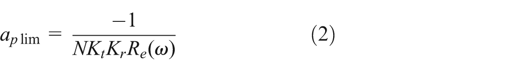
The present milling stability of machine tools can be predicted mainly based on the analytical model developed by Altintas and colleagues^8,9 In their approach, the time-varying force coefficient of the dynamic milling process model was approximated by Fourier-series components. Following this, the stability relationship between the chatter-free axial cutting depths a_plim and the spindle speed n was obtained.

The speed-dependent transfer function H(jω) representing the ratio of the Fourier transform of the displacement X(jω) at the tool tip over the dynamic cutting force F(jω) can be derived by Gagnol et al. ¹⁰ as follows

$$H(j\omega )=\frac{X(j\omega )}{F(j\omega )}=R_e(\omega )+j{I}_m(\omega )$$

(1)

$$a_{plim}=\frac{-1}{N{K}_t{K}_r{R}_e(\omega )}$$

(2)

$$\varphi =\pi -2{\tan }^{-1}\frac{I_m(\omega )}{R_e(\omega )}$$

(3)

$$n=\frac{60\omega }{N(2k\pi +\varphi )},k=\mathrm{lobes}(0,1,2,\dots )$$

(4)

In the above equations, H(jω) = R_e(ω) + jI_m(ω); R_e and I_m are, respectively, the real and imaginary parts of the transfer function of the spindle tool tip. K_t is the cutting force coefficients in the tangential direction to the cutter, and K_r is the ratio of the normal and tangential cutting force coefficient. N is the number of cutter teeth and k is the lobe number.

In a similar way, the chatter-free axial cutting depths a_plim in multiple mode system can be expressed

$$a_{p\lim }=\frac{-1}{N{K}_t{K}_r{R}_e{(\omega )}_r}$$

(5)

r is the number of the modal order; the real part of the transfer function at the rth order modal (R_e(ω) _r ) can be expressed according to the mechanical vibration as follows

$$R_e(\omega {)}_r=\frac{1-{{\omega }_r}^2}{k_r[{(1-{{\omega }_r}^2)}^2+{(2{\zeta }_r{\omega }_r)}^2]}$$

(6)

ω_r = ω/ω_nr is the frequency ratio at the rth order modal, ω is the incentive angular frequency of the milling system, and ω_nr is the natural angular frequency of machine tools at the rth order modal. ${\omega }_{\mathrm{nr}}^2=k_r/m_r$ ; ζ_r = c_r/(2m_rω_nr); m_r, k_r, c_r, and ζ_r are, respectively, modal mass, modal stiffness, modal damping, and modal damping ratio, where k_r = 1/2ζ_r|I_m(ω) _r |. (2ζ_rω_r)² can be ignored because the order of magnitude of ζ_r is usually 10⁻²; when 0 < ω_r < 1 or ω_r > 1, the order of magnitude of (2ζ_rω_r)² is 10⁻⁴–10⁻⁶, which is far smaller than that of (1 − (ω_r)²)². In order to simplify the calculation, equation (5) can be transformed into

$$a_{plim}=\frac{-k_r}{N{K}_t{K}_r}[1-{\left(\frac{\omega }{{\omega }_{\mathrm{nr}}}\right)}^2]$$

(7)

To predict the machining stability, a two-tooth carbide cutter was employed to machine the stock material of Al7075. The radius of cutter is 12 mm, the radial cutting depth is 6 mm, and the milling method is down-milling. The cutting resistance coefficients were calibrated as K_t = 796 N/mm² and K_r = 0.21 by milling experiment. Supposing, machine tool has three order modal parameters (see Table 1) at some position. The stability diagrams of machine tools are shown in Figure 2(a). The zone under the blue straight line is the absolute stable zone. The zone between the blue straight line and the curve is the conditional stable zone. The zone on the curve (the critical values of the axial cutting depth) is the chatter zone. The operators of machine tools often choose the low spindle speed when milling the steel or hard materials. In the meantime, the values of the axial cutting depth in the absolute stable zone are chosen because the conditional stable zone is narrow under low-speed milling. The blue straight line corresponding to the values represent the minimum critical values of the axial cutting depth a_plim(min). As shown in Figure 2(b), the minimum critical values of the axial cutting depth of stable zone under every order modal (blue straight line) change with the values of dynamic stiffness k_dr, where k_dr = 1/|I_m(ω) _r | = 2ζ_rk_r. The minimum critical values of the axial cutting depth of stable zone under second-order modal and multi-modal are consistent basically. The dynamic stiffness under the second-order modal is the lowest (see Table 1). Therefore, the milling stability of machine tools at some position is decided by some order modal parameter which has the lowest dynamic stiffness.

Table 1.

Three order modal parameters of machine tool at some position (assumed values).

Direction	Order	Natural frequency fr (Hz)	Modal stiffness kr (N/m)	Modal damping ratio ζr	Dynamic stiffness kdr (N/m)
X	1	50	5 × 107	0.025	2.5 × 106
Y	2	60	4 × 107	0.021	1.68 × 106
X	3	70	6 × 107	0.023	2.76 × 106

Figure 2.

Stability lobes’ diagrams: (a) zone divisions of stability lobes’ diagram and (b) stability lobes’ diagram under Three order modal parameters.

Establishment of response surface model

The method of response surface can rapidly obtain the functional relationship between independent variable and dependent variable by few test sample data. Generally, the response surface model is the quadratic polynomial model

$$f(X)=k_0+\sum _{i=1}^n{k}_i{x}_i+\sum _{i=1}^n{k}_{\mathrm{ii}}{x}_i^2+\sum _{i=2}^n\sum _{j=1}^{i-1}{k}_{\mathrm{ij}}{x}_i{x}_j$$

(8)

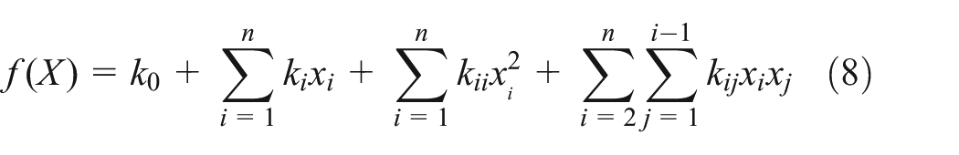
where X = (x₁, x₂,…, x_n) and x_i (i = 1, 2,…, n) are the design variables. k₀, k_i, k_ii, and k_ij are weight coefficients. L = (n + 1)(n + 2)/2 is the number of weight coefficient.

X is the design variable matrix composed by design samples, K is the weight coefficient matrix, and F is the matrix of the minimum critical values of the axial cutting depth obtained by equation (7). ε is the error matrix between the theoretical calculated value F and approximate value F′ calculated by response surface method

$$\mathbf{F}=\mathbf{KX}+\mathbf{\epsilon }=\mathbf{F}\prime +\mathbf{\epsilon }\mathbf{\epsilon }=\mathbf{F}-\mathbf{KX}$$

(9)

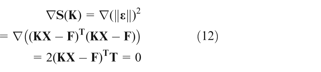
The desired weight coefficient matrix can be obtained by least square method

$$min\mathbf{S}(\mathbf{K})=\Vert \mathbf{\epsilon }{\Vert }^2=(\mathbf{F}-\mathbf{KX}{)}^T(\mathbf{F}-\mathbf{KX})$$

(10)

$$\frac{\delta S(\mathbf{K})}{\delta k_i}=0$$

(11)

$$\begin{array}{c}\multicolumn{1}{c}{\nabla \mathbf{S}(\mathbf{K})=\nabla (\Vert \mathbf{\epsilon }\Vert {)}^2}\\ \multicolumn{1}{c}{=\nabla ({(\mathbf{KX}-\mathbf{F})}^{\mathbf{T}}(\mathbf{KX}-\mathbf{F}))}\\ \multicolumn{1}{c}{=2(\mathbf{KX}-\mathbf{F}{)}^{\mathbf{T}}\mathbf{T}=0}\end{array}$$

(12)

$$\mathbf{K}=({\mathbf{X}}^T\mathbf{X}{)}^{-1}{\mathbf{X}}^{\mathbf{T}}\mathbf{F}$$

(13)

Applied case

Finite element model of machine tools

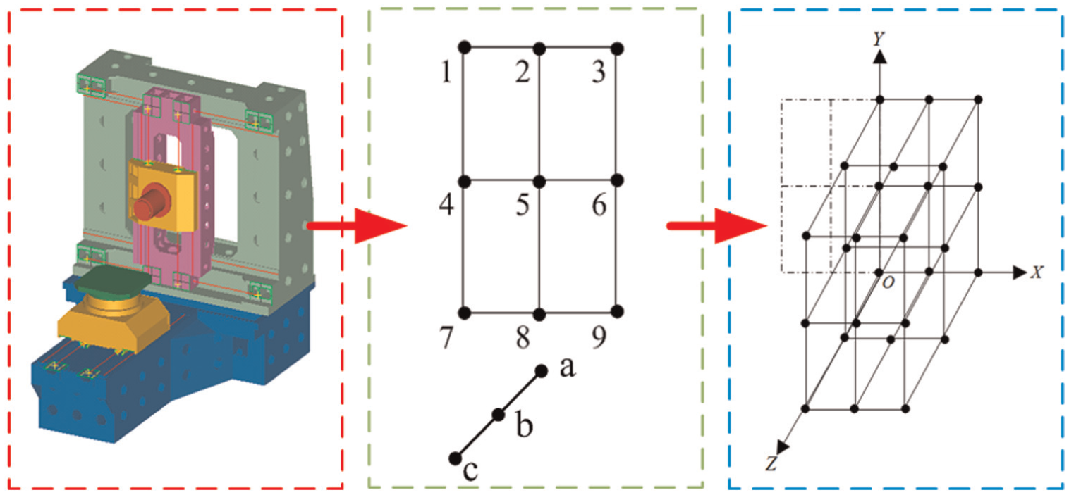
Figure 3 is the three-dimensional computer-aided design (CAD)/computer-aided engineering (CAE) model of the machine tool with box-in-box structure. The column and bed are the fixed parts, and they are connected by bolts. The moving part 1 is composed of the spindle and the spindle box. It can slide on the sliding carriage in the Y-direction. The moving part 2 is composed of the moving part 1 and the sliding carriage. It can slide on the column in the X-direction. The moving part 3 is composed of the worktable and the sliding table. It can slide on the bed in the Z-direction. The transmissions have two types, screw–nut and guide–slider. The key point for accurate modeling of a machine tool structure is the simulation of the interfaces in the above two types of transmissions. The finite element models of the transmissions are shown in Figure 4.

Figure 3.

Three-dimensional CAD/CAE model of machine tool with box-in-box structure.

Figure 4.

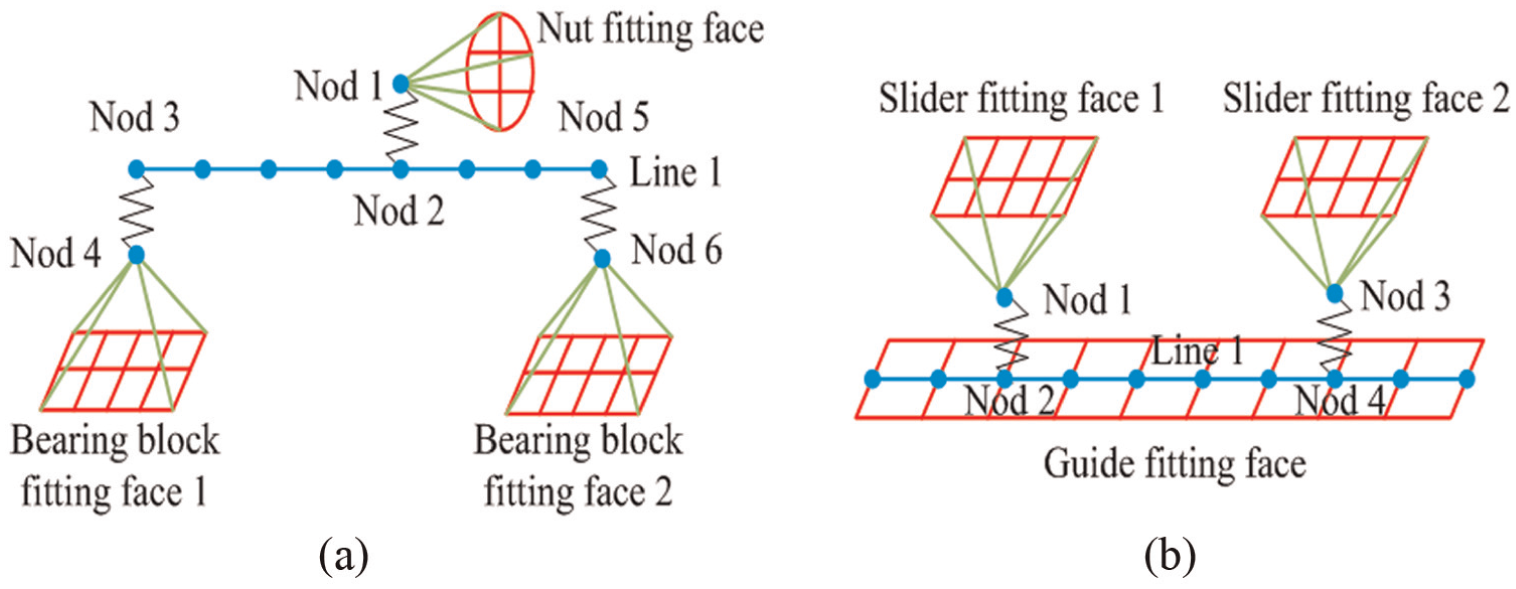
Finite element models of the transmissions: (a) finite element model of screw–nut transmission and (b) finite element model of guide–slider transmission.

Figure 4(a) is the screw–nut transmission. Line 1 is the beam element which represents the screw and Nod 1 represents the nut. The rolling interface between the screw and the nut is composed of Nod 1 and Nod 2 (Nod 2 is on Line 1). Nod 1 and Nod 2 are connected by bushing element which can simulate the spring-damping unit in SAMCEF software. Nod 1 and the nut fitting face are connected by mean element which can simulate mean force transmittance. The bearing element is composed of Nod 3 and Nod 4; Nod 3 is also on Line 1. Nod 4 and the bearing block fitting face 1 are connected by mean element. The same connection way is applicable for Nod 5, Nod 6, and the bearing block fitting face 2.

Figure 4(b) is the guide–slider transmission. Line 1 is the beam element which represents the guide; the guide is fixed on the guide fitting face. Nod 1 represents the slider. The slider and the slider fitting face are connected by mean element. The sliding interface between the guide and slider is composed by Nod 1 and Nod 2 (Nod 2 is on Line 1). Nod 1 and Nod 2 are also connected by bushing element.

The material properties of the components are shown in Table 2 and the stiffness values of interface can be obtained by consulting INA (German INA bearing company) series product manuals according to the work condition (see Table 3). The stiffness of guide–slider interface in feed direction is far smaller than the other two supporting directions and can be identified as 0. The radial stiffness of screw–nut interface is not offered in INA series product manuals; actually, the axial stiffness of screw–nut interface is more concerned, because the radial stiffness is large enough to support the load; in the finite element method (FEM), the degree of freedom in radial direction is constrained, so the radial stiffness of screw–nut interface is marked as “−.” The values of axial stiffness in Table 3 are the values under the preload according to the data offered in product manuals. The axial stiffness and radial stiffness of the bearing fixed in the bearing block are, respectively, 1.81 × 10⁶ and 3.62 × 10⁶ N/m.

Table 2.

Material properties of components.

Name of components	Elasticity modulus (GPa)	Poisson’s ratio	Density (kg/m3)
Column
Bed
Sliding carriageSpindle box	173	0.3	7300
Sliding table
Work table
Screw	219	0.3	7850
Nut	213	0.28	7850
Guide and slider	219	0.3	7850

Table 3.

Stiffness values of interfaces.

Name of interfaces	Stiffness (X-direction) (N/mm)	Stiffness (Y-direction) (N/mm)	Stiffness (Z-direction) (N/mm)
Guide–slider (X-direction)	0	1.31 × 106	1.62 × 106
Guide–slider (Y-direction)	1.72 × 106	0	2.41 × 106
Guide–slider (Z-direction)	1.31 × 106	3.42 × 106	0
Screw–nut (X-direction)	1.26 × 106	–	–
Screw–nut (Y-direction)	–	1.26 × 106	–
Screw–nut (Z-direction)	–	–	1.26 × 106

Division of spatial specific positions

The structure of machine tool on the XOY plane is bilateral symmetrical, so when the moving part 2 is on the left plane of the column, the dynamic characteristics of machine tools are the same as that on the right plane of the column. This study chooses the right plane as the investigated object. Separately set three specific positions (the original point, the middle point, and the end point) on the strokes of the moving part 1, the moving part 2, and the moving part 3. There are totally 27 specific combination positions in the right workspace (see Figure 5).

Figure 5.

Specific combination positions in the right workspace.

The position variables’ groups of moving parts are defined as X = {0,0.5,1}, Y = {0,0.5,1}, and Z = {0,0.5,1}. X represents the ratio of the distance from the moving part 2’s position to the original point and the stroke length. Y represents the ratio of the distance from the moving part 1’s position to the original point and the stroke length. Z represents the ratio of the distance from the moving part 3’s position to the original point and the stroke length. Therefore, the spatial position variables can be expressed as {X,Y,Z} = {(0,0,0), (0,0.5,0), (0,1,0), (0.5,0,0), (0.5,0.5,0), (0.5,1,0), (1,0,0), (1,0.5,0), (1,1,0), (0,0,0.5), (0,0.5,0.5), (0,1,0.5), (0.5,0,0.5), (0.5,0.5,0.5), (0.5,1,0.5), (1,0,0.5), (1,0.5,0.5), (1,1,0.5), (0,0,1), (0,0.5,1), (0,1,1), (0.5,0,1), (0.5,0.5,1), (0.5,1,1), (1,0,1), (1,0.5,1), (1,1,1)}.

Dynamic characteristics of machine tools at different specific positions

One of the key points for accurate simulation of machine tool structural dynamic characteristics is damping values of interface. This article ascertains a uniform damping ratio ζ at some specific position using the method in the literature; ⁴ ζ = 0.024 is obtained by multiple simulation. Figure 6(a) shows the test and measurement instruments of dynamic characteristics of machine tools. Figure 6(b)–(e) shows the analytic and measured results of dynamic characteristics of the machine tool at position b4 (0,1,0.5). The results of simulation and experiment are shown in Table 4. Compared with the results of dynamic characteristics experiment, the error of each order natural frequency and modal stiffness of simulation is controlled in the range of 5% (see Table 4), and that of each order modal damping ratio of simulation is controlled about the range of 10% (see Table 4). The machine tool finite element model can be used in subsequent research. Moreover, dynamic characteristics of machine tools at nine different specific positions have been obtained; the results show that the positions influence on the dynamic characteristics of machine tool at both X- and Y-directions (Figure 7).

Figure 6.

Analytic and measured results of dynamic characteristics of machine tool: (a) test and measurement instruments of dynamic characteristics of machine tool, (b) analytic and measured results of dynamic characteristics of machine tool in X-direction (real part), (c) analytic and measured results of dynamic characteristics of machine tool in X-direction (imaginary part), (d) analytic and measured results of dynamic characteristics of machine tool in Y-direction (real part), and (e) analytic and measured results of dynamic characteristics of machine tool in Y-direction (imaginary part).

Table 4.

Results of simulation and experiment.

Frequency
Order of modal	Mode of vibration	Frequency of experiment (Hz)	Frequency of simulation (Hz)	Error (%)
1	Pitching vibration mode of the column	48.6	51	4.7
2	Yawing vibration mode of the column	56.1	58.3	3.8
3	Bending–torsional coupling mode of the column	81.4	85	4.2
Modal stiffness
Order of modal		Modal stiffness of experiment (N/m)	Modal stiffness of simulation (N/m)	Error (%)
1		9.32 × 107	8.93 × 107	4.4
2		4.9 × 107	5.03 × 107	2.6
3		1.45 × 108	1.43 × 108	1.4
Modal damping ratio
Order of modal		Modal damping ratio of experiment	Modal damping ratio of Simulation	Error (%)
1		0.023	0.025	8
2		0.015	0.017	11.8
3		0.031	0.035	11.4

Figure 7.

Finite element analysis of dynamic characteristics of machine tool at different specific combined positions: (a) finite element analysis of dynamic characteristics of machine tool at different specific combined positions in X-direction (real part), (b) finite element analysis of dynamic characteristics of machine tool at different specific combined positions in X-direction (imaginary part), (c) finite element analysis of dynamic characteristics of machine tool at different specific combined positions in Y-direction (real part), and (d) finite element analysis of dynamic characteristics of machine tool at different specific combined positions in Y-direction (imaginary part).

Establishment of response surface model

The spatial position of machine tools can be shown by three independent variables x, y, and z; each independent variable has three specific values 0, 0.5, and 1. Therefore, three factors and three levels of orthogonal experiment need to be designed. In order to ensure the accuracy of experiment and reduce the cost of computer operation, the Box–Behnken ¹¹ response surface design method is chosen in this study. Figure 8 is the Box–Behnken model; the central points of space and edges are the experimental design points. Table 5 is the orthogonal test table of three levels and three factors based on Box–Behnken method.

Figure 8.

Box–Behnken design model for three levels.

Table 5.

Orthogonal test table of three levels and three factors.

Test No.	x	Y	z	aplim(min) (mm)
1	0.5	0.5	0.5	5.08
2	0.5	0.5	0.5	5.08
3	1	0.5	0	5.12
4	0.5	0.5	0.5	5.08
5	0	0.5	1	5.1
6	0	1	0.5	5.28
7	0.5	0.5	0.5	5.08
8	0	0.5	0	5.1
9	1	1	0.5	5.3
10	0.5	1	0	4.66
11	1	0	0.5	4.54
12	0.5	0	0	4.54
13	0.5	0.5	0.5	5.08
14	0.5	0	1	4.55
15	0.5	1	1	5.28
16	0	0	0.5	4.53
17	1	0.5	1	5.12

X, which is the design variables’ matrix composed by design samples, and F, which is the matrix of the minimum critical values of the axial cutting depth, can be expressed as

$$\mathbf{X}=\left[\begin{array}{cccccccc}\hfill 0.5\hfill & \hfill 0.5\hfill & \hfill 0.5\hfill & \hfill 0.25\hfill & \hfill 0.25\hfill & \hfill 0.25\hfill & \hfill 0.25\hfill & \hfill 0.25\hfill \\ \multicolumn{1}{c}{0.5}& \hfill 0.5\hfill & \hfill 0.5\hfill & \hfill 0.25\hfill & \hfill 0.25\hfill & \hfill 0.25\hfill & \hfill 0.25\hfill & \hfill 0.25\hfill \\ \multicolumn{1}{c}{1}& \hfill 0.5\hfill & \hfill 0\hfill & \hfill 0\hfill & \hfill 0\hfill & \hfill 1\hfill & \hfill 0.25\hfill & \hfill 0\hfill \\ \multicolumn{1}{c}{0.5}& \hfill 0.5\hfill & \hfill 0.5\hfill & \hfill 0.25\hfill & \hfill 0.25\hfill & \hfill 0.25\hfill & \hfill 0.25\hfill & \hfill 0.25\hfill \\ \multicolumn{1}{c}{0}& \hfill 0.5\hfill & \hfill 1\hfill & \hfill 0\hfill & \hfill 0.5\hfill & \hfill 0\hfill & \hfill 0.25\hfill & \hfill 1\hfill \\ \multicolumn{1}{c}{0}& \hfill 1\hfill & \hfill 0.5\hfill & \hfill 0\hfill & \hfill 0.5\hfill & \hfill 0\hfill & \hfill 1\hfill & \hfill 0.25\hfill \\ \multicolumn{1}{c}{0.5}& \hfill 0.5\hfill & \hfill 0.5\hfill & \hfill 0.25\hfill & \hfill 0.25\hfill & \hfill 0.25\hfill & \hfill 0.25\hfill & \hfill 0.25\hfill \\ \multicolumn{1}{c}{0}& \hfill 0.5\hfill & \hfill 0\hfill & \hfill 0\hfill & \hfill 0\hfill & \hfill 0\hfill & \hfill 0.25\hfill & \hfill 0\hfill \\ \multicolumn{1}{c}{1}& \hfill 1\hfill & \hfill 0.5\hfill & \hfill 0.5\hfill & \hfill 0.5\hfill & \hfill 1\hfill & \hfill 1\hfill & \hfill 0.25\hfill \\ \multicolumn{1}{c}{0.5}& \hfill 1\hfill & \hfill 0\hfill & \hfill 0\hfill & \hfill 0\hfill & \hfill 0.25\hfill & \hfill 1\hfill & \hfill 0\hfill \\ \multicolumn{1}{c}{1}& \hfill 0\hfill & \hfill 0.5\hfill & \hfill 0.5\hfill & \hfill 0\hfill & \hfill 1\hfill & \hfill 0\hfill & \hfill 0.25\hfill \\ \multicolumn{1}{c}{0.5}& \hfill 0\hfill & \hfill 0\hfill & \hfill 0\hfill & \hfill 0\hfill & \hfill 0.25\hfill & \hfill 0\hfill & \hfill 0\hfill \\ \multicolumn{1}{c}{0.5}& \hfill 0.5\hfill & \hfill 0.5\hfill & \hfill 0.25\hfill & \hfill 0.25\hfill & \hfill 0.25\hfill & \hfill 0.25\hfill & \hfill 0.25\hfill \\ \multicolumn{1}{c}{0.5}& \hfill 0\hfill & \hfill 1\hfill & \hfill 0.5\hfill & \hfill 0\hfill & \hfill 0.25\hfill & \hfill 0\hfill & \hfill 1\hfill \\ \multicolumn{1}{c}{0.5}& \hfill 1\hfill & \hfill 1\hfill & \hfill 0.5\hfill & \hfill 1\hfill & \hfill 0.25\hfill & \hfill 1\hfill & \hfill 1\hfill \\ \multicolumn{1}{c}{0}& \hfill 0\hfill & \hfill 0.5\hfill & \hfill 0\hfill & \hfill 0\hfill & \hfill 0\hfill & \hfill 0\hfill & \hfill 0.25\hfill \\ \multicolumn{1}{c}{1}& \hfill 0.5\hfill & \hfill 1\hfill & \hfill 1\hfill & \hfill 0.5\hfill & \hfill 1\hfill & \hfill 0.25\hfill & \hfill 1\hfill \end{array}\right],\mathbf{F}=\left[\begin{array}{c}\hfill 5.08\hfill \\ \multicolumn{1}{c}{5.08}\\ \multicolumn{1}{c}{5.12}\\ \multicolumn{1}{c}{5.08}\\ \multicolumn{1}{c}{5.1}\\ \multicolumn{1}{c}{5.28}\\ \multicolumn{1}{c}{5.08}\\ \multicolumn{1}{c}{5.1}\\ \multicolumn{1}{c}{5.3}\\ \multicolumn{1}{c}{4.66}\\ \multicolumn{1}{c}{4.54}\\ \multicolumn{1}{c}{4.54}\\ \multicolumn{1}{c}{5.08}\\ \multicolumn{1}{c}{4.55}\\ \multicolumn{1}{c}{5.28}\\ \multicolumn{1}{c}{4.53}\\ \multicolumn{1}{c}{5.12}\end{array}\right]$$

According to equation (13), the weight coefficient matrix K can be obtained as follows: $\mathbf{K}=[\begin{array}{cccccccc}\hfill -2.36\hfill & \hfill 0.32\hfill & \hfill 1.1\hfill & \hfill 0.01\hfill & \hfill 4.61\hfill & \hfill 2.37\hfill & \hfill -3.04\hfill & \hfill -2.25\hfill \end{array}]$ ; the constant term is 5.12.

Therefore, writing to the form of equation (8), the functional expression of response surface model with the relationship between the position and the value of minimum critical axial cutting depth can be expressed as

$$\begin{array}{cc}\multicolumn{1}{c}{a_{plim(min)}(x,y,z)}& =f(x,y,z)\hfill \\ \multicolumn{1}{c}{}& =5.12-2.36x+0.32y+1.1z\hfill \\ \multicolumn{1}{c}{}& +0.01\mathrm{xz}+4.61\mathrm{yz}\hfill \\ \multicolumn{1}{c}{}& +2.37x^2-3.04y^2-2.25z^2\hfill \end{array}$$

(14)

The quality verification equation is expressed as

$$R^2=1-\frac{\sum _{i=1}^m{(f_i-f_i^{\prime })}^2}{\sum _{i=1}^m{(f_i-f_i^{″})}^2}$$

(15)

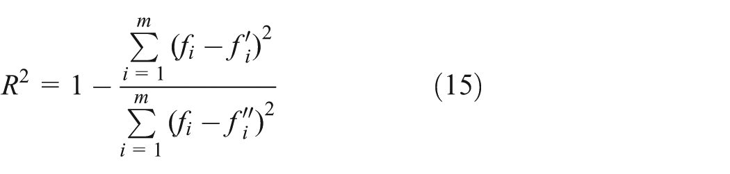
where m is the number of the samples, $f_i^{\prime }$ is the value of response surface calculation, f_i is the value of finite element calculation, and $f_i^{″}$ is the average value of finite element calculation. R² → 1 indicates high fitting accuracy. The values calculated on six non-specific positions are used to verify the fitting precision of the established response surface model. In this model, R² = 0.7405. The accuracy of established response surface model is high enough for application (see Table 6).

Table 6.

Minimum critical values of the axial cutting depth at non-specific combined positions.

x	y	z	$f_i^{\prime }$ (mm)	fi (mm)	$f_i^{″}$ (mm)	R 2
0.2	0.4	0	4.38	4.52	4.99	0.7405
0.4	0.2	0.4	4.94	5.13
0.3	0.6	0.6	5.23	5.01
0.6	0.3	0.5	5.05	4.97
0.5	0.7	1	5.34	5.51
0.7	0.1	0.3	4.89	4.80

Evaluation of machine tool with position-dependent milling stability

Figure 9 shows the minimum critical values of the axial cutting depth in right half workspace. It is a four-dimensional chart. The color indicates the different minimum critical values of the axial cutting depth. For the machine tool with box-in-box structure, the variation in the minimum critical values of the axial cutting depth is obvious; the variation range is from 1.8 to 6 mm. The obvious variation in the milling stability is not the satisfied design for machine tools. The optimal design is that the milling stability is conformed at any position; certainly, it is hardly to be realized. Therefore, the designer had better make the variation of the milling stability stable as much as possible to reach the productivity goals for machine tools. In other words, the structural stiffness of machine tools should be reinforced at the position where the milling stability is weak.

Figure 9.

Minimum critical values of the axial cutting depth in right half workspace.

Figure 10 shows the minimum critical values of the axial cutting depth when the worktable is separately at three specific positions. The variation in the minimum critical values of the axial cutting depth is obvious when the worktable is at the original point of the stroke (Z = 0). The variation range is from 2 to 5 mm. The minimum critical values of the axial cutting depth at the positions close to the left-down and right-down corners of the XOY plane are large and the values at the positions close to the top of the XOY plane are small. The variation in the minimum critical values of the axial cutting depth is not obvious when the worktable is at the middle of the stroke (Z = 0.5). The variation range is from 4.2 to 5.6 mm. The minimum critical values of the axial cutting depth at the positions close to the left and right sides of the XOY plane are large and the values at the positions close to the top and bottom of the XOY plane are small. The variation in the minimum critical values of the axial cutting depth is also obvious when the worktable is at the end of the stroke (Z = 1). The variation range is from 3.5 to 6 mm. The minimum critical values of the axial cutting depth at the positions close to the left-top and right-top corners of the XOY plane are large and the values at the positions close to the bottom of the XOY plane are small.

Figure 10.

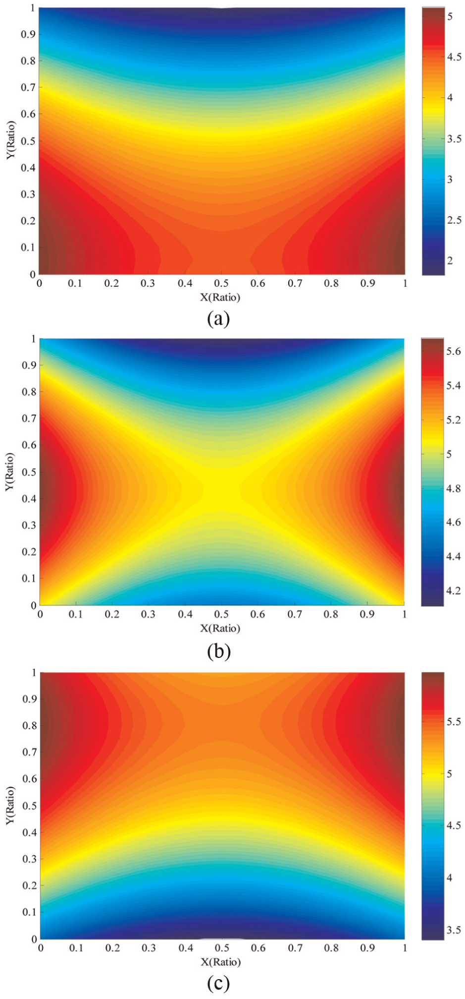
Minimum critical values of the axial cutting depth at three specific positions: (a) minimum critical values of the axial cutting depth in XOY plane, when Z = 0; (b) minimum critical values of the axial cutting depth in XOY plane, when Z = 0.5; and (c) minimum critical values of the axial cutting depth in XOY plane, when Z = 1.

Above all, according to the variation in the minimum critical values of the axial cutting depth in the whole workspace, the designer can rapidly evaluate the milling stability of machine tools. The weak positions of machine tools can be found out. Then, by modifying the structures, the dynamic characteristics of machine tools can be reinforced.

Conclusion

The milling stability is one of the important evaluation criterions of dynamic characteristics of machine tools. In this article, a finite element modeling technique including simulation of sliding and rolling interfaces was presented. This technique can be applied to predict the milling stability of the machine tools with box-in-box structure. The established response surface model can show the relationship between the position and the value of minimum critical axial cutting depth at any position in the whole workspace. The precision of the response surface model is illustrated and the model can be used to rapidly evaluate the milling stability of machine tools with position dependence. The results of the stability analysis clearly demonstrate the dependence of the milling stability of machine tools at different positions. When the worktable and the sliding table are separate at three specific positions, the milling stability in the XOY plane has a bigger variation and the values of the minimum critical axial cutting depth at the positions close to the top of the column are small. It is necessary to reinforce the structural stiffness at these positions according to the results shown in the figures. This method of rapid evaluation of machine tools with position-dependent stability can be easily utilized to optimize machine tools’ structure to obtain suitable dynamic characteristics of machine tools.