Benchmark solutions for two-dimensional fluid flow and heat transfer problems in irregular regions using multigrid method

Abstract

In the previous researches about the benchmark solutions in the irregular regions, there are some obvious shortcomings, such as small number of computational grids, simple computational domain, small characteristic number, and lack of mixed convection benchmark solution. In order to improve this situation, this article deeply studied the benchmark solutions for two-dimensional fluid flow and heat transfer problems in the irregular regions under the body-fitted coordinate system. Taking the lid-driven flow, natural convection, and mixed convection problems as the research objects and considering the influence of boundary configurations of the computational domains, Reynolds number, Prandtl number, and Grashof number, this article designed three groups of test cases. The program code is first verified through employing the nonlinear multigrid method based on the collocated finite volume method and then the numerical solutions of three test cases with 1024 × 1024 grids and convergence criterion of 10⁻¹⁴ are obtained to get the benchmark solutions estimated by the Richardson extrapolation method.

Introduction

The fluid flow and heat transfer phenomena in practice always happen in the irregular regions, so how to achieve the accurate and efficient calculations of fluid flow and heat transfer problems in the irregular regions is no doubt of great importance. Currently, many articles published in the international academic journals are related to the numerical simulations of the fluid flow and heat transfer problems in the irregular regions. Thus, in order to verify the calculation results and provide references for different algorithms, it is quite necessary to study the benchmark solutions of fluid flow and heat transfer problems defined in the irregular regions. As one of the popular methods to discretize the irregular regions, the body-fitted coordinate grids have been widely used due to its good applicability and desirable ability to follow the boundaries, ¹ which is mainly applied to internal flows over smoothly varying irregular boundaries. Therefore, this article aims to research on the benchmark solutions of fluid flow and heat transfer problems in the two-dimensional (2D) irregular regions with the body-fitted coordinate grids.

As a basic research topic, the benchmark solutions have been studied and reported systematically by researchers all over the world, especially the lid-driven flow^2,3 and natural convection^4,5 in a square cavity, and the calculated benchmark solutions have already been verified and proved. For the benchmark solutions in the irregular regions, the cases in the literature usually can be solved by utilizing the cylindrical coordinate system ⁶ or polar coordinate system, ⁷ but the method using the body-fitted coordinate system is rarely proposed. The limited literatures involving these issues are as follows: in the literature, Demirdzic et al. ⁸ showed the benchmark solutions of the lid-driven flow in an inclined square cavity with the angles of 30° and 45°, natural convection in a 45° inclined square cavity, and a cylinder which is enclosed by a square duct. The Reynolds number is set to be 100 and 1000, respectively, in the case of lid-driven flow; the Prandtl number is set to be 0.1 and 10, respectively, while Rayleigh number is 10⁶ in the case of natural convection. In that article, the multigrid (MG) method based on the collocated finite volume method (FVM) is used and coupling between pressure and velocity is treated by SIMPLE algorithm. And the benchmark solutions with 320 × 320 grids are given. Besides, Oosterlee et al. ⁹ tested the correctness of the algorithm through comparing the results in the literature ⁸ and presented the benchmark solutions of L-shaped lid-driven cavity flow with 256 × 256 grids and Reynolds number of 100 and 1000. Different from the literature, ⁸ Oosterlee et al. ⁹ employed the symmetric coupled alternating lines (SCAL) to deal with the coupling between pressure and velocity and solved the discretized equations by the means of nonlinear MG method based on the staggered FVM.

Although the literature^8,9 has studied the benchmark solutions of 2D lid-driven cavity flow and natural convection in the irregular regions, there is still some room for improvement. For example, the maximum number of grids in the literature ⁸ is only 320 × 320 in which case the numerical results may still be affected by the discretization error. And the maximum Reynolds number in the literature^8,9 is only 1000 and there is no research regarding the problems with high Reynolds number. In addition, the configurations in previous researches are relatively simple to indicate the influence of boundary shape on the accuracy and robustness of the numerical simulation. To the best knowledge of the authors, there are also no such literatures studying the benchmark solutions of mixed convection problems under the body-fitted coordinate system. Therefore, in order to improve this situation, this article aims to research on the benchmark solutions for 2D fluid flow and heat transfer problems in the irregular regions under the body-fitted coordinate system using MG method.

The layout of this article is organized as follows. In section “Test cases,” the reasons and purposes to design the test cases are explained in detail, and the dimensionless general governing equations as well as the calculation conditions are given in this section. In section “Numerical methods,” we mainly focus on the numerical methods for solving the test cases. In section “Program testing,” the correctness of algorithms is tested through comparing the calculation results of lid-driven flow and natural convection with those in the literature. ⁸ On this basis, section “Benchmark solutions” shows the benchmark solutions of different test cases under various calculation conditions. In the final section, the most important findings of this study are summarized.

Test cases

Description of test cases

This article takes three typical cases of fluid flow and heat transfer problems, lid-driven flow, natural convection, and mixed convection, to be the research objects, noting them as test cases 1–3, respectively. The computational domains of the three test cases all contain the irregular configurations shown in Figure 1 where l = 1 m. The reasons and purposes of designing the three test cases are as follows:

1. Because previous literature did not discuss the benchmark solutions of the mixed convection problem under the body-fitted coordinate system, this article designs this kind of case to expand the application scope of the benchmark solutions.

2. The boundary shapes in the literature^8,9 are relatively simple. To investigate the influence of the boundary shape on the numerical accuracy, this article designs the regions with non-parallel east–west boundaries as shown in Figure 1(b) and (c). The function of the west boundary shape in Figure 1(c) is $x(y)=0.1\sin [\pi -2\pi (y/l)]$ .

Figure 1.

Sketch map of the irregular computational domains: (a) parallelogram cavity, (b) trapezoid cavity, and (c) sine-type cavity.

To guarantee the reliability of the benchmark solutions, this article first compared the numerical results of lid-driven flow on the domain shown in Figure 1(a) with the reference results in the literature ⁸ to verify the reliability and accuracy of the present algorithms and code and then utilizes the solid program to carry out the subsequent numerical calculations.

Dimensionless general governing equations and calculation conditions

Different from the literature,^8,9 this article first applies the dimensionless method to the governing equations of the physical problems in test cases 1–3. The dimensionless treatment can not only make the numerical results more universal but also cover the magnitude gap between different physical variables to enhance the numerical accuracy and reduce the constant calculations in the governing equations. For the sake of concision, the details of dimensionless method are not provided.

In the physical plane x–y, the 2D dimensionless unsteady convection–diffusion equation of the incompressible fluid is given as

$$\begin{array}{c}\multicolumn{1}{c}{\frac{\partial \Phi }{\partial \tau }+\frac{\partial (U\Phi )}{\partial X}+\frac{\partial (V\Phi )}{\partial Y}=\frac{\partial }{\partial X}\left({\Gamma }^{*}\frac{\partial \Phi }{\partial X}\right)}\\ \multicolumn{1}{c}{+\frac{\partial }{\partial Y}\left({\Gamma }^{*}\frac{\partial \Phi }{\partial Y}\right)+R(X,Y)}\end{array}$$

(1)

where $\Phi$ , ${\Gamma }^{*}$ , and $R(X,Y)$ take different values in different test cases.

Since the computational domains in Figure 1 are all irregular regions, this article transforms the dimensionless governing equation (1) in the physical plane x–y into the computational plane $\xi -\eta$ for solution and the following governing equation can be obtained (Appendix 2)

$$\begin{array}{c}\multicolumn{1}{c}{\frac{\partial \Phi }{\partial \tau }+\frac{1}{J^{*}}\frac{\partial (U^{*}\Phi )}{\partial \xi }+\frac{1}{J^{*}}\frac{\partial (V^{*}\Phi )}{\partial \eta }}\\ \multicolumn{1}{c}{=\frac{1}{J^{*}}\frac{1}{\partial \xi }[\frac{{\Gamma }^{*}}{J^{*}}({\alpha }^{*}{\Phi }_{\xi }-{\beta }^{*}{\Phi }_{\eta })]}\\ \multicolumn{1}{c}{+\frac{1}{J^{*}}\frac{1}{\partial \eta }[\frac{{\Gamma }^{*}}{J^{*}}({\gamma }^{*}{\Phi }_{\eta }-{\beta }^{*}{\Phi }_{\xi })]+S(\xi ,\eta )}\end{array}$$

(2)

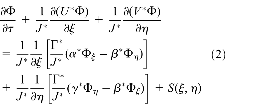
As shown in Tables 1 and 2, when $\Phi$ , ${\Gamma }^{*}$ , and $S(\xi ,\eta )$ in equation (2) take different values, the dimensionless governing equations of lid-driven flow, natural convection, and mixed convection can be represented, respectively. Table 3 provides the dimensionless boundary conditions and calculation conditions of test cases 1–3.

Table 1.

Parameters of the continuity equation and energy equation.

Test cases	Physical problems	Continuity equation			Energy equation
		$\Phi$	${\Gamma }^{*}$	$S(\xi ,\eta )$	$\Phi$	${\Gamma }^{*}$	$S(\xi ,\eta )$
1	Lid-driven flow	1	0	0	–	–	–
2	Natural convection	1	0	0	$\Theta$	1/Pr	0
3	Mixed convection	1	0	0	$\Theta$	1/Pr/Re	0

Table 2.

Parameters of the momentum equations.

Test cases	Physical problems	x—momentum equation			y—momentum equation
		$\Phi$	${\Gamma }^{*}$	$S(\xi ,\eta )$	$\Phi$	${\Gamma }^{*}$	$S(\xi ,\eta )$
1	Lid-driven flow	U	1/Re	$(P_{\eta }{Y}_{\xi }-P_{\xi }{Y}_{\eta })/J^{*}$	V	1/Re	$(P_{\xi }{X}_{\eta }-P_{\eta }{X}_{\xi })/J^{*}$
2	Natural convection	U	1	$(P_{\eta }{Y}_{\xi }-P_{\xi }{Y}_{\eta })/J^{*}$	V	1	$(P_{\xi }{X}_{\eta }-P_{\eta }{X}_{\xi })/J^{*}+\mathrm{Gr}\Theta$
3	Mixed convection	U	1/Re	$(P_{\eta }{Y}_{\xi }-P_{\xi }{Y}_{\eta })/J^{*}$	V	1/Re	$(P_{\xi }{X}_{\eta }-P_{\eta }{X}_{\xi })/J^{*}+\mathrm{Ri}\Theta$

Table 3.

Dimensionless boundary conditions and calculation conditions of test cases 1–3.

Test cases	Physical problems	Dimensionless boundary conditions	Dimensionless calculation conditions
1	Lid-driven flow	North: U = 1, V = 0; else: U = V = 0	Re = 100, 1000, 5000
2	Natural convection	West: Θh = 1; east: Θc = 0; else: adiabatic	Pr = 0.1, 10; Ra = 106
3	Mixed convection	North: U = 1, V = 0; else: U = V = 0 West: Θh = 1; east: Θc = 0; else: adiabatic	Gr = 106, 107; Pr = 0.71; Re = 1000

Numerical methods

In order to guarantee the conservation of the dimensionless governing equation (2), this article applies the FVM to solve the three physical problems. The second-order central difference scheme is employed to discretize the convection term and diffusion term. The deferred correction technology is used for the discretization of the convection term to better meet the diagonal dominant condition of coefficient matrix of the discretized equations. To further satisfy the conservation of flux, the coupling between pressure and velocity is treated by the SIMPLE algorithm on collocated grids, where the dimensionless contravariant U* and V* are selected as the velocity components of the continuity equation in the computational plane and dimensionless U and V are selected as the velocity components of the momentum equations. The cross-derivative terms in the continuity equation and momentum equations caused by the non-orthogonality of grids are treated as the source terms. To make the programming easier, this article utilizes the additional source term method to deal with the boundary conditions of the governing equation.

To obtain the high-resolution numerical solutions and reduce the influence of discretization errors on the numerical results, the computational domain in computational plane is divided into 1024 × 1024 uniform grids. And the convergence criterion is strictly set as the absolute residuals of the continuity equation less than 10⁻¹⁴. The governing equations hold high nonlinearity because the lid-driven flow, natural convection, and mixed convection are all the multi-variable coupling problems. Besides, the number of computational grids is also large for 1024 × 1024 grids adopted. As a result, the above factors would lead to the slow convergence rate of the computation process. To speed up computation, this article adopts the nonlinear MG method based on collocated FVM for the solution where the full approximation scheme (FAS) is chosen as the nonlinear version of the MG method. In FAS, V-cycle is adopted and strong implicit procedure (SIP) method is employed to solve the discretized equations. It is not necessary to obtain the precise solutions on coarse grid when MG method is adopted. Thus, the convergence criterion is only set on the finest mesh, while on other grid levels the number of smoothing is given. On the coarse grid, the numbers of pre-smoothing and post-smoothing for solving the momentum equations and energy equation are both set as 4, and set as 12 for solving the pressure correction equation. In the calculation, grid levels are determined by the coarsest grid number, which is set as 16 × 16 in lid-driven flow and natural convection and 64 × 64 in mixed convection, respectively. The under-relaxation factors for different test cases are as follows: the velocity and pressure under-relaxation factors in the case of lid-driven flow are 0.7 and 0.2, respectively; the velocity, pressure, and temperature under-relaxation factors in the cases of natural convection and mixed convection are 0.4, 0.1, and 0.5, respectively.

To prove the computational efficiency of MG method, a set of numerical results such as computational cost, convergence rate, and convergence ratio in the computation of lid-driven flow in parallelogram cavity with Re = 100 on 1024 × 1024 grids are provided in Tables 4 and 5. Table 4 shows the computational cost for solving U-momentum equation, V-momentum equation, and P-correction equation, respectively, in a V-cycle of MG method. In Table 5, the convergence rate and convergence ratio are provided. The convergence rate is the maximum residual after each V-cycle, and the convergence ratio gives the ratio of residual of successive V-cycles. From the results, it can be seen that MG method is a wise choice in the present computation.

Table 4.

Computational cost of a V-cycle ( ${\upsilon }_1$ , ${\upsilon }_2$ ).

Equation	${\upsilon }_1$ (Pre-smoothing)	${\upsilon }_2$ (Post-smoothing)	WU
U-momentum equation	4	4	32/3
V-momentum equation	4	4	32/3
P-correction equation	12	12	32

WU: work unit.

Table 5.

Convergence rate and ratio.

V-cycle	Convergence rate	Ratio	V-cycle	Convergence rate	Ratio
1	6.990 × 10−6	–	21	1.208 × 10−12	0.676
2	9.949 × 10−7	0.142	22	8.424 × 10−13	0.697
3	2.815 × 10−7	0.283	23	5.943 × 10−13	0.705
4	5.989 × 10−8	0.213	24	4.047 × 10−13	0.681
5	6.862 × 10−9	0.115	25	2.769 × 10−13	0.684
6	2.019 × 10−9	0.294	26	1.946 × 10−13	0.703
7	4.303 × 10−10	0.213	27	1.334 × 10−13	0.686
8	2.050 × 10−10	0.476	28	9.029 × 10−14	0.677
9	1.202 × 10−10	0.586	29	6.163 × 10−14	0.683
10	7.887 × 10−11	0.656	30	4.262 × 10−14	0.692
11	5.211 × 10−11	0.661	31	2.840 × 10−14	0.666
12	3.070 × 10−11	0.589	32	1.983 × 10−14	0.698
13	2.179 × 10−11	0.710	33	1.337 × 10−14	0.674
14	1.504 × 10−11	0.690	34	9.013 × 10−15	0.674
15	1.007 × 10−11	0.670	35	6.272 × 10−15	0.696
16	7.457 × 10−12	0.741	36	4.120 × 10−15	0.657
17	5.246 × 10−12	0.704	37	2.807 × 10−15	0.681
18	3.492 × 10−12	0.666	38	1.928 × 10−15	0.687
19	2.528 × 10−12	0.724	39	1.262 × 10−15	0.655
20	1.786 × 10−12	0.706	40	8.692 × 10−16	0.689

Program testing

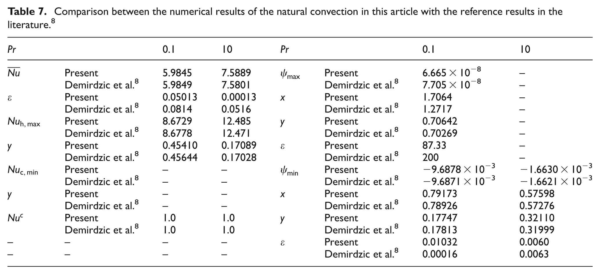
In this section, the numerical results of lid-driven flow and natural convection are first given, and then the comparisons between the present numerical results and the reference results in the literature ⁸ are conducted to verify the accuracy and reliability of the algorithms in this article, as shown in Tables 6 and 7 and Figure 2.

Table 6.

Comparison between the numerical results of the lid-driven flow in this article with the reference results in the literature. ⁸

$\beta ={45}^{\circ }$		Re = 100		Re = 1000
		Minimum	Maximum	Minimum	Maximum
$\psi$	Present	−7.0233 × 10−2	3.6735 × 10−5	−5.3480 × 10−2	1.0025 × 10−2
	Demirdzic et al. 8	−7.0226 × 10−2	3.6831 × 10−5	−5.3507 × 10−2	1.0039 × 10−2
x	Present	1.1136	0.34118	1.3150	0.77970
	Demirdzic et al. 8	1.1100	0.33867	1.3130	0.77663
y	Present	0.54621	0.14294	0.57383	0.39982
	Demirdzic et al. 8	0.54638	0.14308	0.57404	0.39851
$\epsilon$	Present	1.4238 × 10−3	0.48455	2.2438 × 10−2	9.9751 × 10−2
	Demirdzic et al. 8	2.1941 × 10−2	1.3555	0.10689	0.33133

Table 7.

Comparison between the numerical results of the natural convection in this article with the reference results in the literature. ⁸

Pr		0.1	10	Pr		0.1	10
$\overline{\mathrm{Nu}}$	Present	5.9845	7.5889	${\psi }_{max}$	Present	6.665 × 10−8	–
	Demirdzic et al. 8	5.9849	7.5801		Demirdzic et al. 8	7.705 × 10−8	–
$\epsilon$	Present	0.05013	0.00013	x	Present	1.7064	–
	Demirdzic et al. 8	0.0814	0.0516		Demirdzic et al. 8	1.2717	–
$N{u}_{\mathrm{h},\max }$	Present	8.6729	12.485	y	Present	0.70642	–
	Demirdzic et al. 8	8.6778	12.471		Demirdzic et al. 8	0.70269	–
y	Present	0.45410	0.17089	$\epsilon$	Present	87.33	–
	Demirdzic et al. 8	0.45644	0.17028		Demirdzic et al. 8	200	–
$N{u}_{\mathrm{c},\min }$	Present	–	–	${\psi }_{min}$	Present	−9.6878 × 10−3	−1.6630 × 10−3
	Demirdzic et al. 8	–	–		Demirdzic et al. 8	−9.6871 × 10−3	−1.6621 × 10−3
y	Present	–	–	x	Present	0.79173	0.57598
	Demirdzic et al. 8	–	–		Demirdzic et al. 8	0.78926	0.57276
$N{u}^c$	Present	1.0	1.0	y	Present	0.17747	0.32110
	Demirdzic et al. 8	1.0	1.0		Demirdzic et al. 8	0.17813	0.31999
–	–	–	–	$\epsilon$	Present	0.01032	0.0060
–	–	–	–		Demirdzic et al. 8	0.00016	0.0063

Figure 2.

Comparison between the velocity profiles along centerlines CL1 and CL2 for the lid-driven flow in this article with the reference results in the literature: ⁸ (a) U and (b) V.

From Table 6, Figure 2, and Table 7, it can be clearly seen that the numerical results in this article meet very well with the reference results in the literature, ⁸ and the numerical accuracy of the maximum Nusselt number and stream function values is higher than that in the literature. ⁸ In addition, the curves of U and V velocity profiles all go through the 15 selected points of the previous benchmark solutions in the literature. ⁸ Through the above comparisons, it can be reasonably concluded that the proposed algorithms are reliable and accurate to ensure the subsequent numerical calculations.

Benchmark solutions

In section “Program testing,” the algorithm in this article has been verified by the lid-driven flow and natural convection in the parallelogram cavity. In the following text, the benchmark solutions of the lid-driven flow, natural convection, and mixed convection will be calculated on the computational domains with 1024 × 1024 grids. The detailed calculation conditions are presented in Table 3 of section “Test cases.”

Lid-driven flow

The numerical results of lid-driven flow with Reynolds number of 100 and 5000 are given below. Figure 3 is the streamlines for the lid-driven flow. It can be clearly seen that there is substantial difference between the contour map of Re = 5000 with that of Re = 100. To be specific, the first vortex of Re = 5000 is much smaller than that of Re = 100 and it is concentrated on the top right corner of the computational domain. However, the second vortex of Re = 5000 is bigger than that of Re = 100 and it fills about three-fourths of the whole cavity. The reason for this result is that the driving force increases along with the Reynolds number and the fluid movement also becomes more intense. Thus, when the first vortex gets smaller, the second vortex has larger development space and the more intense fluid flow further enhances the full development of the second vortex. It can also be observed that the number of vortex increases with Reynolds number: when Re = 100, there is only one main vortex and it fills almost the whole cavity; but when Re = 5000, there are three to five vortexes which means the fluid flow has been fully developed. Figure 3(a)–(c) shows different development trends of the vortexes and the reason is the different computational domains and boundary shapes, leading to the vortex development in different spaces. Figure 3 presents the fourth and fifth vortexes of the streamline which also suggests the high accuracy of this algorithm.

Figure 3.

Streamlines for the lid-driven flow when Re = 100 and Re = 5000: (a) parallelogram cavity, (b) trapezoid cavity, and (c) sine-type cavity.

Table 8 presents the minimum and maximum stream function values in vortex center and their position for the lid-driven flow on 1024 × 1024 grids. And Figure 4 shows the V velocity profile at the centerline CL1 for the sake of qualitative comparison. Table 9 lists the selected values estimated by the Richardson extrapolation method for quantitative description of the V velocity profiles in Figure 4.

Table 8.

Minimum and maximum stream function values in vortex center and their position for the lid-driven flow on 1024 × 1024 grids.

Re	Computational domain	${\psi }_{min}(x,y)$	${\psi }_{max}(x,y)$
100	(a) Parallelogram cavity	−7.0233 × 10−2 (1.1136, 0.54621)	3.6735 × 10−5 (0.34118, 0.14294)
	(b) Trapezoid cavity	−0.10679 (1.4521, 0.45230)	1.4545 × 10−4 (2.0880, 0.14294)
	(c) Sine-type cavity	−0.10331 (0.67577, 0.75684)	1.1283 × 10−4 (0.11441, 0.067383)
5000	(a) Parallelogram cavity	−3.0620 × 10−2 (1.5075, 0.63736)	1.8087 × 10−2 (0.82502, 0.36115)
	(b) Parallelogram cavity	−9.3950 × 10−2 (1.5477, 0.37082)	1.6333 × 10−2 (0.81884, 0.35701)
	(c) Sine-type cavity	−5.1708 × 10−2 (1.0282, 0.87402)	2.9199 × 10−2 (0.43119, 0.59278)

Figure 4.

V velocity profile for the lid-driven flow along the centerline CL1: (a) parallelogram cavity, (b) trapezoid cavity, and (c) sine-type cavity.

Table 9.

Selected values of the velocity profiles in Figure 4.

No.	(a) Parallelogram cavity				(b) Trapezoid cavity				(c) Sine-type cavity
	Re = 100		Re = 5000		Re = 100		Re = 5000		Re = 100		Re = 5000
	X	V	X	V	X	V	X	V	X	V	X	V
1	0.48344	1.6186 × 10−2	0.41508	−1.8421 × 10−4	0.50799	1.5314 × 10−2	0.47175	−3.4113 × 10−2	4.4320 × 10−2	5.3153 × 10−2	8.2171 × 10−3	−3.8986 × 10−2
2	0.54398	3.5563 × 10−2	0.45414	−1.9243 × 10−2	0.63077	5.6115 × 10−2	0.54368	−8.7201 × 10−2	9.3018 × 10−2	9.8201 × 10−2	2.4288 × 10−2	−8.4306 × 10−2
3	0.61429	6.2448 × 10−2	0.47758	−4.3275 × 10−2	0.76163	9.9909 × 10−2	0.68847	−3.5995 × 10−2	0.14710	0.13119	6.3752 × 10−2	−0.12707
4	0.68656	8.6198 × 10−2	0.49906	−6.8651 × 10−2	0.91364	0.12618	0.98339	4.9650 × 10−2	0.23148	0.14703	0.15101	−8.7493 × 10−2
5	0.76859	9.7719 × 10−2	0.54203	−9.5177 × 10−2	1.0651	0.14262	1.1151	8.0769 × 10−2	0.33628	0.12928	0.23336	−5.9787 × 10−2
6	0.85658	8.3862 × 10−2	0.60258	−6.8461 × 10−2	1.2274	0.13826	1.1557	0.19369	0.42581	9.3143 × 10−2	0.35119	−2.5592 × 10−2
7	0.91704	5.8394 × 10−2	0.68461	−4.0638 × 10−2	1.3303	0.10065	1.1775	0.31039	0.50462	4.6436 × 10−2	0.48392	1.0627 × 10−2
8	0.99516	7.7321 × 10−3	0.77445	−1.3768 × 10−2	1.4529	1.0866 × 10−3	1.2211	0.43781	0.58225	−1.2722 × 10−2	0.55186	2.9230 × 10−2
9	1.0479	−3.5782 × 10−2	0.87603	1.5303 × 10−2	1.5325	−0.10356	1.3272	0.29213	0.63192	−5.6805 × 10−2	0.61086	4.6041 × 10−2
10	1.0889	−7.0897 × 10−2	0.97367	4.3142 × 10−2	1.5873	−0.18602	1.6133	−8.5184 × 10−2	0.68778	−0.10953	0.67425	6.5122 × 10−2
11	1.1416	−0.11559	1.0245	5.7900 × 10−2	1.6394	−0.26420	1.8006	−0.33026	0.75397	−0.16658	0.73247	8.3464 × 10−2
12	1.2315	−0.15747	1.0928	6.9327 × 10−2	1.7190	−0.32817	1.8564	−0.39765	0.84683	−0.20658	0.78736	9.2441 × 10−2
13	1.2940	−0.12382	1.1592	5.6567 × 10−2	1.7937	−0.27462	1.8955	−0.50935	0.91515	−0.17121	0.85882	7.3202 × 10−2
14	1.3174	−8.7798 × 10−2	1.2061	3.3967 × 10−2	1.8423	−0.19617	1.9243	−0.26227	0.95174	−0.11736	0.91110	4.3631 × 10−2
15	1.3389	−4.1316 × 10−2	1.2745	6.2552 × 10−3	1.9170	−7.7765 × 10−2	1.9830	2.0729 × 10−2	0.98454	−4.3339 × 10−2	0.97016	1.0041 × 10−2

Natural convection

This section shows the numerical results of natural convection with Pr = 10, Pr = 0.1, and Ra = 10⁶. Figure 5 is the streamlines for the natural convection. We can see that there is only one main vortex when the Prandtl number is set to be 10 and 0.1, filling almost the whole computational domain with slight difference for the same area. The more intense flow when Pr = 0.1 than that when Pr = 10 leads to the full development of the main vortex. It is obvious that Prandtl number has great influence on the shape of main vortex. Table 10 shows the minimum and maximum stream function values in vortex center and their position on 1024 × 1024 grids in Figure 5.

Figure 5.

Streamlines for the natural convection when Ra = 10⁶: (a) parallelogram cavity, (b) trapezoid cavity, and (c) sine-type cavity.

Table 10.

Minimum and maximum stream function values in vortex center and their position for the natural convection on 1024 × 1024 grids.

Pr	Computational domain	${\psi }_{min}(x,y)$	${\psi }_{max}(x,y)$
10	(a) Parallelogram cavity	−1.6630 (0.57598, 0.32110)	6.5367 × 10−5 (1.7064, 0.70642)
	(b) Trapezoid cavity	−1.9128 (0.59000, 0.32110)	1.4335 × 10−3 (1.9771, 0.43711)
	(c) Sine-type cavity	−2.0131 (0.85625, 0.59668)	7.9361 × 10−3 (1.1201, 0.70801)
0.1	(a) Parallelogram cavity	−96.874 (0.91733, 0.52964)	6.6645 × 10−3 (1.7064, 0.70642)
	(b) Trapezoid cavity	−123.80 (1.5217, 0.20924)	0.43428 (0.78068, 0.058696)
	(c) Sine-type cavity	−129.71 (0.53512, 0.79004)	0.56866 (1.1483, 0.75684)

Figure 6 is the isotherms for the natural convection when Ra = 10⁶. It is shown that the isotherms are always vertical to the adiabatic boundaries, but for the same computational domain the curvature of isotherms differs from each other. When Pr = 0.1, the isotherms in the center of cavity have larger curvature than those when Pr = 10, since when the Prandtl number is getting smaller, the heat diffusion ability of fluid flow becomes stronger than the momentum diffusion ability which results in the great buoyancy force. The convective movement between the cool and warm fluids becomes more intense, leading to the better mixing between fluids with different temperature.

Figure 6.

Isotherms for the natural convection when Ra = 10⁶: (a) parallelogram cavity, (b) trapezoid cavity, and (c) sine-type cavity.

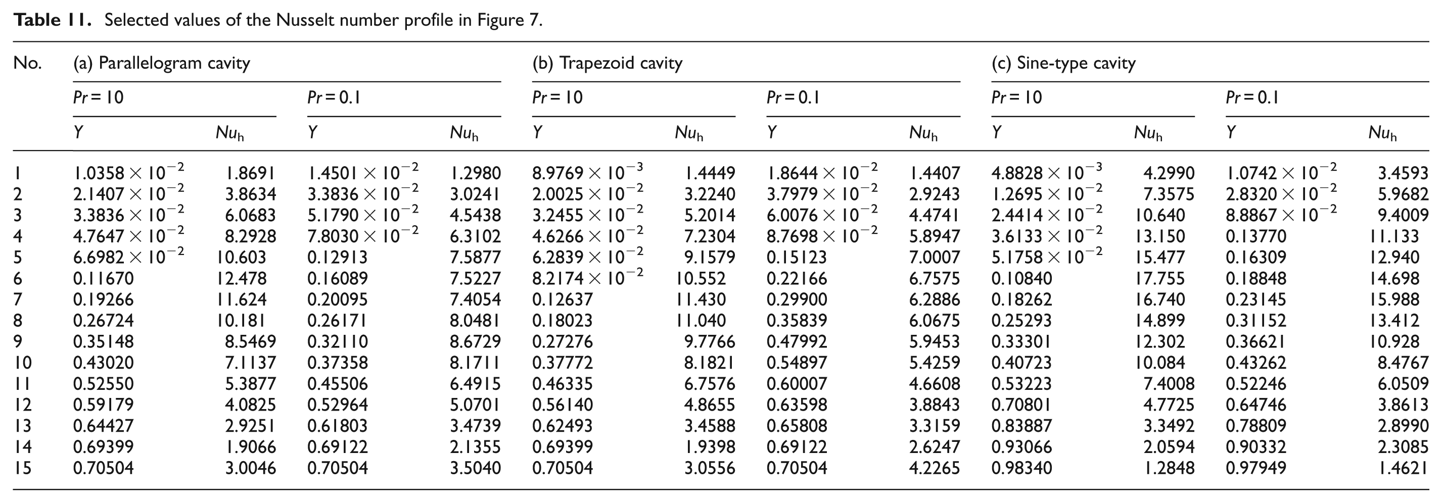
Figure 7 shows the Nusselt number along the hot wall when Ra = 10⁶ with Pr = 10 and Pr = 0.1. Table 11 presents the selected values of the Nusselt number profiles in Figure 7. It is worth pointing out that the coordinate value Y of the selected points is the actual coordinate rather than the length of the hot wall.

Figure 7.

Nusselt number along the hot wall for the natural convection when Ra = 10⁶: (a) parallelogram cavity, (b) trapezoid cavity, and (c) sine-type cavity.

Table 11.

Selected values of the Nusselt number profile in Figure 7.

No.	(a) Parallelogram cavity				(b) Trapezoid cavity				(c) Sine-type cavity
	Pr = 10		Pr = 0.1		Pr = 10		Pr = 0.1		Pr = 10		Pr = 0.1
	Y	Nu h	Y	Nu h	Y	Nu h	Y	Nu h	Y	Nu h	Y	Nu h
1	1.0358 × 10−2	1.8691	1.4501 × 10−2	1.2980	8.9769 × 10−3	1.4449	1.8644 × 10−2	1.4407	4.8828 × 10−3	4.2990	1.0742 × 10−2	3.4593
2	2.1407 × 10−2	3.8634	3.3836 × 10−2	3.0241	2.0025 × 10−2	3.2240	3.7979 × 10−2	2.9243	1.2695 × 10−2	7.3575	2.8320 × 10−2	5.9682
3	3.3836 × 10−2	6.0683	5.1790 × 10−2	4.5438	3.2455 × 10−2	5.2014	6.0076 × 10−2	4.4741	2.4414 × 10−2	10.640	8.8867 × 10−2	9.4009
4	4.7647 × 10−2	8.2928	7.8030 × 10−2	6.3102	4.6266 × 10−2	7.2304	8.7698 × 10−2	5.8947	3.6133 × 10−2	13.150	0.13770	11.133
5	6.6982 × 10−2	10.603	0.12913	7.5877	6.2839 × 10−2	9.1579	0.15123	7.0007	5.1758 × 10−2	15.477	0.16309	12.940
6	0.11670	12.478	0.16089	7.5227	8.2174 × 10−2	10.552	0.22166	6.7575	0.10840	17.755	0.18848	14.698
7	0.19266	11.624	0.20095	7.4054	0.12637	11.430	0.29900	6.2886	0.18262	16.740	0.23145	15.988
8	0.26724	10.181	0.26171	8.0481	0.18023	11.040	0.35839	6.0675	0.25293	14.899	0.31152	13.412
9	0.35148	8.5469	0.32110	8.6729	0.27276	9.7766	0.47992	5.9453	0.33301	12.302	0.36621	10.928
10	0.43020	7.1137	0.37358	8.1711	0.37772	8.1821	0.54897	5.4259	0.40723	10.084	0.43262	8.4767
11	0.52550	5.3877	0.45506	6.4915	0.46335	6.7576	0.60007	4.6608	0.53223	7.4008	0.52246	6.0509
12	0.59179	4.0825	0.52964	5.0701	0.56140	4.8655	0.63598	3.8843	0.70801	4.7725	0.64746	3.8613
13	0.64427	2.9251	0.61803	3.4739	0.62493	3.4588	0.65808	3.3159	0.83887	3.3492	0.78809	2.8990
14	0.69399	1.9066	0.69122	2.1355	0.69399	1.9398	0.69122	2.6247	0.93066	2.0594	0.90332	2.3085
15	0.70504	3.0046	0.70504	3.5040	0.70504	3.0556	0.70504	4.2265	0.98340	1.2848	0.97949	1.4621

Mixed convection

In order to expand the application scope of benchmark solutions, this article also studied the mixed convection problem. The mixed convection can be regarded as the combination between the lid-driven flow and natural convection; the driving forces of the fluid come from the force of the moving boundary as well as the buoyancy force. In the following text, the numerical results of mixed convection when Gr = 10⁶, Gr = 10⁷, and Pr = 0.71 are provided.

Figure 8 is the streamlines for the mixed convection. It can be observed from Figure 8 that along with the increase in Grashof number, the number of vortex does not change but the shape changes a lot. When Gr = 10⁶, there is only one main vortex and the shape of the main vortex is concentric deformed circles which fill almost two-thirds of the cavity. When Gr = 10⁷, there is still one main vortex, but the shape is bigger than that of Gr = 10⁶ and presents as long strips which almost fill the whole region. The reason is that along with the increase in Grashof number, the intensity of natural convection becomes larger and the natural convection is dominant. In addition, the shape of streamlines when Gr = 10⁶ is similar to that in the lid-driven flow when Re = 1000. Because when Gr = 10⁶ and Re = 1000, the Ri = 1, which signifies that the influences of lid-driven flow and natural convection on the fluid flow are almost the same. The minimum and maximum stream function values in vortex center and their position are given in Table 12.

Figure 8.

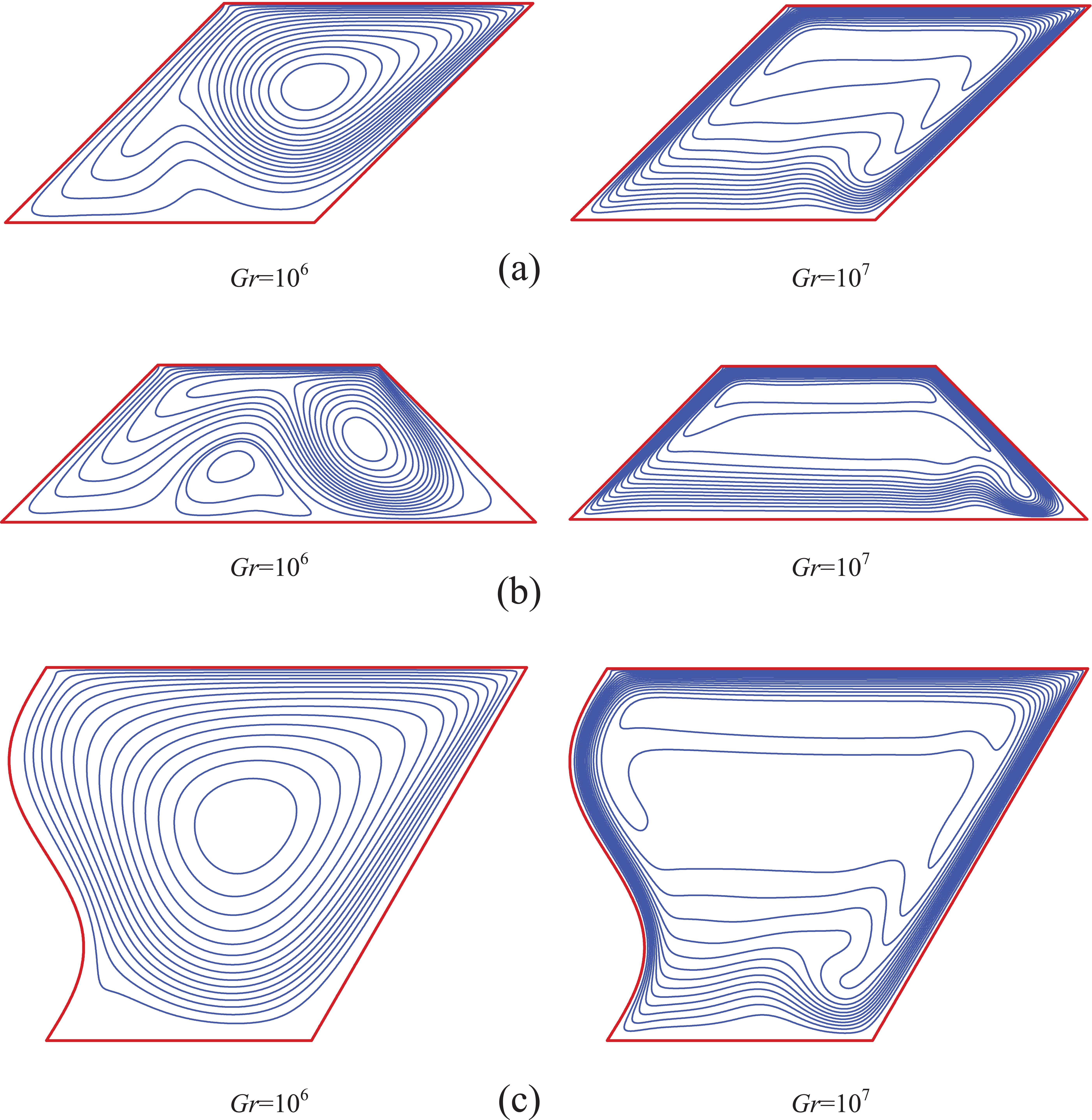
Streamlines for the mixed convection when Re = 1000 and Pr = 0.71: (a) parallelogram cavity, (b) trapezoid cavity, and (c) sine-type cavity.

Table 12.

Minimum and maximum stream function values in vortex center and their position for the mixed convection on 1024 × 1024 grids.

Gr	Computational domain	${\psi }_{min}(x,y)$	${\psi }_{max}(x,y)$
106	(a) Parallelogram cavity	−7.3303 × 10−2 (0.99553, 0.43987)	2.0847 × 10−6 (0.66082, 0.017263)
	(b) Trapezoid cavity	−7.5875 × 10−2 (1.6385, 0.37358)	3.2094 × 10−3 (1.0374, 0.25895)
	(c) Sine-type cavity	−9.9861 × 10−2 (0.53176, 0.58106)	2.0090 × 10−4 (1.1280, 0.72168)
107	(a) Parallelogram cavity	−4.3156 × 10−2 (0.81818, 0.59455)	–
	(b) Trapezoid cavity	−4.4498 × 10−2 (1.4432, 0.59041)	1.7084 × 10−5 (1.7962, 0.61803)
	(c) Sine-type cavity	−4.9690 × 10−2 (0.67010, 0.87207)	1.7900 × 10−4 (1.1426, 0.74707)

Figure 9 is the isotherms for the mixed convection when Re = 1000 and Pr = 0.71. It is shown that for different domains with various boundary shapes, the isotherms differ from each other greatly when Gr = 10⁶ and Gr = 10⁷. When Gr = 10⁶, the isotherms show the shape of vortex, while Gr = 10⁷, the shape of isotherms is similar to that of natural convection when Gr = 10⁶. The reason for this phenomenon is the dominance of natural convection, and lid-driven flow on the mixed convection varies along with the different Grashof numbers. Although the three computational domains are quite different from each other, the isotherms are always vertical to the adiabatic boundaries. For the same calculation region, the curvature of isotherms when Gr = 10⁶ is larger than that when Gr = 10⁷, since the contour shape of the former situation is affected by lid-driven flow while the latter one is mainly influenced by the buoyancy force.

Figure 9.

Isotherms for the mixed convection when Re = 1000 and Pr = 0.71: (a) parallelogram cavity, (b) trapezoid cavity, and (c) sine-type cavity.

Figure 10 shows the Nusselt number along the hot wall for the mixed convection when Re = 1000 and Pr = 0.71. Table 13 gives the selected values of the Nusselt number profiles in Figure 10.

Figure 10.

Nusselt number along the hot wall for the mixed convection when Re = 1000 and Pr = 0.71: (a) parallelogram cavity, (b) trapezoid cavity, and (c) sine-type cavity.

Table 13.

Selected values of the Nusselt number profiles in Figure 10.

No.	(a) Parallelogram cavity				(b) Trapezoid cavity				(c) Sine-type cavity
	Gr = 106		Gr = 107		Gr = 106		Gr = 107		Gr = 106		Gr = 107
	Y	Nu h	Y	Nu h	Y	Nu h	Y	Nu h	Y	Nu h	Y	Nu h
1	1.3120 × 10−2	1.9742	6.2148 × 10−3	4.0968	1.5882 × 10−2	1.7477	4.8337 × 10−3	2.9214	8.7891 × 10−3	4.0493	2.9297 × 10−3	7.9453
2	2.9693 × 10−2	4.4612	1.1739 × 10−2	7.7408	3.5217 × 10−2	3.8647	1.0358 × 10−2	6.2571	2.4414 × 10−2	7.1968	6.8359 × 10−3	12.867
3	4.6266 × 10−2	6.8283	1.8644 × 10−2	12.197	5.3171 × 10−2	5.6946	1.7263 × 10−2	10.364	4.7852 × 10−2	10.312	1.0742 × 10−2	16.617
4	6.9744 × 10−2	9.4620	2.4169 × 10−2	15.457	7.9411 × 10−2	7.6846	2.4169 × 10−2	14.128	9.8633 × 10−2	12.521	1.8555 × 10−2	22.401
5	0.12637	11.590	3.3836 × 10−2	19.902	0.13742	9.0590	3.3836 × 10−2	18.206	0.13770	12.691	2.6367 × 10−2	26.325
6	0.19956	11.199	6.1458 × 10−2	23.986	0.21890	8.7115	6.5601 × 10−2	22.144	0.19629	14.336	5.1758 × 10−2	30.172
7	0.27690	10.266	0.11808	22.021	0.28519	8.2854	0.11394	20.571	0.26855	16.219	0.14551	26.765
8	0.37082	8.8252	0.17194	19.935	0.36667	7.8010	0.18161	18.306	0.33496	14.737	0.23926	24.171
9	0.44263	7.9969	0.26171	17.038	0.44401	7.3716	0.28105	15.786	0.39941	11.992	0.32910	20.403
10	0.52412	7.9197	0.33629	14.869	0.51030	7.0268	0.39706	13.042	0.46582	9.5520	0.41699	16.631
11	0.59317	8.1339	0.41639	12.769	0.59317	6.6283	0.49097	10.949	0.56934	7.1845	0.51074	13.441
12	0.63598	8.0511	0.51445	10.576	0.67051	6.3763	0.57245	9.3693	0.70996	5.6730	0.65332	10.043
13	0.67741	8.0512	0.63184	8.2813	0.69261	7.5164	0.64565	7.8759	0.85059	5.7747	0.81348	8.2968
14	0.69675	10.179	0.68984	6.6669	0.70089	9.8151	0.68984	6.6097	0.95801	5.7656	0.92480	6.9442
15	0.70504	13.705	0.70504	8.8848	0.70504	11.252	0.70504	8.8075	0.98730	7.4977	0.97949	5.3119

Conclusion

This article studied the benchmark solutions of the lid-driven flow, natural convection, and mixed convection in 2D irregular regions under the body-fitted coordinate system. On the basis of verifying the reliability and correctness of the algorithms, this article employed the nonlinear MG method based on the collocated FVM to solve the above physical problems on 1024 × 1024 grids under different calculation conditions. Based on the numerical results, the following conclusions can be obtained:

1. The results of lid-driven flow in parallelogram cavity verified the reliability of the present method and proved it to be more accurate than the benchmark solutions in the literature. ⁸

2. The benchmark solutions of lid-driven flow and natural convection on 1024 × 1024 grids are given and this article also studied the influence of boundary shape, Reynolds number, Prandtl number, and Grashof number on the numerical results.

3. The benchmark solutions of the mixed convection are presented to expand the application scope of the benchmark solutions.