Analytical and numerical solutions of squeezing nanofluid flow between parallel plates: A comparison of IRPSM and HPM

Abstract

The nanofluid flow between two parallel plates has many applications across various fields of engineering. The addition of nanoparticles to conventional fluids can improve the rheological properties of nanofluids, enhance the heat transfer rate, and have other beneficial characteristics. Therefore, a squeezing flow problem between two parallel plates has been investigated in this article. The nanofluid flow is composed of alumina (Al₂O₃) nanoparticles and water, which is used as a base fluid. This study is featured according to the recommendations of a previous study to implement the improved residual power series method (IRPSM). The mathematical model is presented in the form of partial differential equations (PDEs), which are then transformed into ordinary differential equations (ODEs) by means of similarity variables. The considered problem is solved by two analytical methods called IRPSM, the homotopy perturbation method (HPM), and a numerical method (NDSolve). The residual errors of both applied techniques are compared to verify the validation of a new method. The comparison of both applied analytical techniques is conducted at the 17th order of approximations. From the obtained results, we confirmed that both techniques are in great agreement and have a very close relationship. The results of both methods are compared with the numerical method, and it was found that the absolute error between the IRPSM and numerical techniques is much more significant than the absolute error between the HPM and numerical techniques. Also, we have seen that the residuals of IRPSM are quite significant in terms of less residual errors than those of HPM. We confirmed that the IRPSM is a more powerful method than the HPM in terms of solving such types of mathematical problems.

Introduction

Differential equations, whether partial or ordinary, are used to model scientific problems. Typically, these equations cannot be solved analytically; thus, unique methods must be used to solve them. The recently established techniques, including the perturbation approach, to build an analytical solution to these equations have received a lot of attention recently. Techniques for perturbation rely too heavily on the so-called “small parameters.” Therefore, it becomes sense to create some novel analytical methods that are not depending on little factors.

Homotopy perturbation method (HPM), which was proposed by He, ¹ is one of the most powerful technique to solve nonlinear differential equations. Various mathematical models have been solved by authors in many scientific fields.^2–4 The HPM is always valid whether a small physical parameter exists or not. HPM expresses the solution of a differential equation in a form of summation of an infinite series. Furthermore, in order to get the solutions, this technique relies on certain initial guesses for the differential operators. It should be highlighted that false results might arise if these initial guesses are selected in an improper manner. As shown by Ariel, ² Pamuk and Pamuk, ³ and Aly and Ebaid, ⁵ the approach does, nonetheless, provide accurate solutions in a large cases where effective initial estimates have been made. Panda et al. ⁶ presented the application of HPM in heat and mass transfer across a rectangular fin. Mallick et al. ⁷ presented the applications of HPM to investigate the unknown thermal factors in an annular fin.

Improved Residual Power Series Method (IRPSM) is the improved version of the residual power series method (RPSM). The idea of RPSM was introduced by Arqub. ⁸ This method is more effective in construction of power series solutions for the linear and nonlinear differential equations. RPSM has no need of linearization, discretization, or perturbation. It is important to note that the RPSM is only applicable for the solution of initial value problems. Based on these observations, Khan et al. ⁹ extended this method for the solutions of boundary valued problems which we then called IRPSM. They compared the results of IRPSM with the results of optimal homotopy analysis method (OHAM), differential transform method (DTM) and exact solutions of the problems they considered. They found that the results of IRPSM are more significant than the other methods and hence an improved version of the RPSM is introduced. Following this method, Dawar et al. ¹⁰ introduced it in the field of fluid dynamics. They solved a thin film flow problem over a thin film planar surface. They compared their results with the published results^11–14 and have found a good agreement among all the methods.

According to the future recommendations of Dawar et al., ¹⁰ it is intended in this effort to solve a squeezing flow problem between two parallel plates. Therefore, the nanofluid flow comprising alumina (Al₂O₃) nanoparticles between two parallel plates is considered in this effort. It is also intended to compare the IRPSM and HPM results to get more effective results from this study. Both the IRPSM and HPM will be tested at 17th order of approximations to confirm the validity of both techniques. Also, the residual errors of both techniques will tell us about the most powerful method to solve such types of mathematical problems. Therefore, to conduct a comparative analysis, we have presented this paper in section-wise. The mathematical formulation of the problem under consideration is presented in Section “Model formulation.” Basic ideas of the HPM and IRPSM are introduced in Sections “Fundamentals of HPM” and “Fundamentals of IPRMS,” respectively. A comparative analysis between HPM and IRPSM is presented in Section “Comparison of numerical, IRPSM, and HPM solutions.” The results obtained by IRPMS and their physical discussion are presented in Section “Results and discussion.” The final remarks are listed in Section “Conclusions and future scope.”

Model formulation

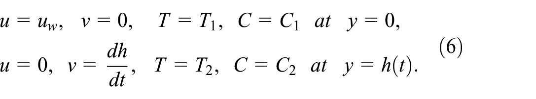
Assume a laminar and time-dependent flow of nanofluid comprising alumina (Al₂O₃) nanoparticles between two parallel plates. Water is considered to be a base fluid. The two plates are placed in such a way that the lower plate locates at $x-$ axis and $y-$ axis remains vertical to the lower plate as shown in Figure 1. The two plates are separated to each other at a distance $y=h\left(t\right)=\sqrt{\frac{{\upsilon }_f(1-\alpha t)}{a}}$ such that $(1-\alpha t)>0$ where $\alpha$ and $a$ are the constants (non-negative). The two plates are squeezes for $\alpha >0$ until they touches $t=1/\alpha$ and for $\alpha <0$ , the two plates separates. It is also assumed that the upper plate moves toward the lower plates with velocity $v=\frac{\mathrm{dh}}{\mathrm{dt}}$ . The lower plate is maintained at a constant temperature $T_1$ and concentration $C_1$ . Similarly, the upper plate is maintained at a constant temperature $T_2$ and concentration $C_2$ . The impact of heat source/sink is taken into consideration to investigate the heat transfer rate. The impacts of magnetic field, Joule heating, and viscous dissipation are ignored. Thus, the leading equations are defined as^15,16:

Figure 1.

Geometrical representation of the flow problem.

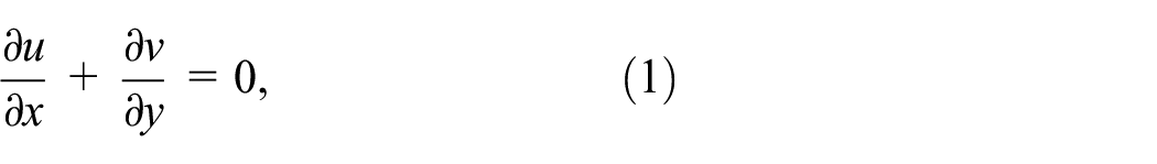
Continuity equation

$$\frac{\partial u}{\partial x}+\frac{\partial v}{\partial y}=0,$$

(1)

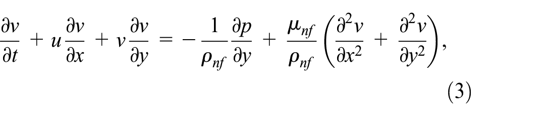
Momentum equations

$$\frac{\partial u}{\partial t}+u\frac{\partial u}{\partial x}+v\frac{\partial u}{\partial y}=-\frac{1}{{\rho }_{\mathrm{nf}}}\frac{\partial p}{\partial x}+\frac{{\mu }_{\mathrm{nf}}}{{\rho }_{\mathrm{nf}}}(\frac{{\partial }^{2}u}{\partial x^2}+\frac{{\partial }^{2}u}{\partial y^2}),$$

(2)

$$\frac{\partial v}{\partial t}+u\frac{\partial v}{\partial x}+v\frac{\partial v}{\partial y}=-\frac{1}{{\rho }_{\mathrm{nf}}}\frac{\partial p}{\partial y}+\frac{{\mu }_{\mathrm{nf}}}{{\rho }_{\mathrm{nf}}}(\frac{{\partial }^{2}v}{\partial x^2}+\frac{{\partial }^{2}v}{\partial y^2}),$$

(3)

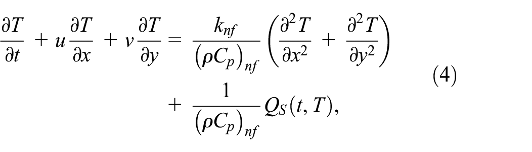
Energy equation

$$\begin{array}{c}\multicolumn{1}{c}{\frac{\partial T}{\partial t}+u\frac{\partial T}{\partial x}+v\frac{\partial T}{\partial y}=\frac{k_{\mathrm{nf}}}{{\left(\rho C_p\right)}_{\mathrm{nf}}}(\frac{{\partial }^{2}T}{\partial x^2}+\frac{{\partial }^{2}T}{\partial y^2})}\\ +\frac{1}{{\left(\rho C_p\right)}_{\mathrm{nf}}}{Q}_S(t,T),\hfill \end{array}$$

(4)

where $Q_S(t,T)=\frac{Q_0(T-T_2)}{(1-\alpha t)}$ .

Concentration equation

$$\frac{\partial C}{\partial t}+u\frac{\partial C}{\partial x}+v\frac{\partial C}{\partial y}=D_B(\frac{{\partial }^{2}C}{\partial x^2}+\frac{{\partial }^{2}C}{\partial y^2}),$$

(5)

with boundary conditions:

$$\begin{array}{c}u=u_w,v=0,T=T_1,C=C_1\mathrm{at}y=0,\hfill \\ u=0,v=\frac{\mathrm{dh}}{\mathrm{dt}},T=T_2,C=C_2\mathrm{at}y=h\left(t\right).\hfill \end{array}$$

(6)

The thermophysical relations are defined as:

$$\begin{array}{c}{\mu }_{\mathrm{nf}}=\frac{{\mu }_f}{{(1-\varphi )}^{2.5}},{\left(\rho C_p\right)}_{\mathrm{nf}}=(1-\varphi ){\left(\rho C_p\right)}_f+\varphi {\left(\rho C_p\right)}_s,\hfill \\ {\rho }_{\mathrm{nf}}=(1-\varphi ){\rho }_f+\varphi {\rho }_s,k_{\mathrm{nf}}=\frac{k_s+2k_f-2\varphi (k_f-k_s)}{k_s+2k_f+\varphi (k_f-k_s)}.\hfill \end{array}$$

(7)

The thermophysical properties of the base fluid and nanoparticle are defined in Table 1.

Table 1.

Thermophysical properties of the base fluid and nanoparticle. ¹⁷

Properties	$\begin{array}{l}\rho \\ \left[\mathrm{kg}.{\mathrm{m}}^{-3}\right]\end{array}$	$\begin{array}{l}{C}_p\\ \left[\mathrm{J}.{\mathrm{kg}}^{-1}.{\mathrm{K}}^{-1}\right]\end{array}$	$\begin{array}{l}k\\ \left[\mathrm{W}.{\mathrm{m}}^{-1}.{\mathrm{K}}^{-1}\right]\end{array}$	$\begin{array}{l}\sigma \\ \left[\mathrm{\Omega }.{\mathrm{m}}^{-1}\right]\end{array}$
Water	997.1	4179	0.613	0.05
Al2O3	3970	765	40	5.96 × 107

The similarity variables are defined as^15,16:

$$\begin{array}{c}u=\frac{\mathrm{ax}}{(1-\alpha t)}f\prime \left(\xi \right),v=-\sqrt{\frac{a{\upsilon }_f}{1-\alpha t}}f\left(\xi \right),\hfill \\ \theta \left(\xi \right)=\frac{T-T_2}{T_1-T_2},\varphi \left(\xi \right)=\frac{C-C_2}{C_1-C_2},\xi =y\sqrt{\frac{a}{{\upsilon }_f(1-\alpha t)}}.\hfill \end{array}$$

(8)

The transformed ordinary differential equations are obtained as:

$$\frac{Z_1}{Z_2}{f}^{\mathrm{iv}}\left(\xi \right)+(f\left(\xi \right)-S\xi )f″\prime \left(\xi \right)-3\mathrm{Sf}″\left(\xi \right)-f\prime \left(\xi \right)f″\left(\xi \right)=0,$$

(9)

$$\frac{Z_3}{Z_4}\theta ″\left(\xi \right)+\mathrm{Pr}(f\left(\xi \right)-S\xi )\theta \prime \left(\xi \right)+\frac{Q\mathrm{Pr}}{Z_4}\theta \left(\xi \right)=0,$$

(10)

$$\varphi ″\left(\xi \right)+\mathrm{Sc}(f\left(\xi \right)-S\xi )\varphi \prime \left(\xi \right)=0,$$

(11)

with boundary conditions:

$$\begin{array}{c}f(\xi =0)=0,f\prime (\xi =0)=1,\theta (\xi =0)=1,\varphi (\xi =0)=1,\hfill \\ f(\xi =1)=S,f\prime (\xi =1)=0,\theta (\xi =1)=0,\varphi (\xi =1)=0.\hfill \end{array}$$

(12)

In the above equations $Z_1(={\mu }_{\mathrm{nf}}/{\mu }_f)$ , $Z_2(={\rho }_{\mathrm{nf}}/{\rho }_f)$ , $Z_3(=k_{\mathrm{nf}}/k_f)$ , $Z_4(={\left(\rho C_p\right)}_{\mathrm{nf}}/{\left(\rho C_p\right)}_f)$ , $\mathrm{Sc}(=\frac{{\nu }_f}{D_B})$ is the Schmidt number, $S(=\frac{\alpha }{2a})$ is the unsteady squeezing parameter, $Q\left(=\frac{Q_0}{a{\left(\rho C_p\right)}_f}\right)$ is the heat source factor, and $\mathrm{Pr}(=\frac{{\mu }_f{\left(C_p\right)}_f}{k_f})$ is the Prandtl number.

The physical quantities of interest like skin friction ( $C_f$ ), Nusselt number ( $\mathrm{Nu}$ ), and Sherwood number ( $\mathrm{Sh}$ ) are defined as:

$$\begin{array}{c}{C}_f=\frac{{\mu }_{\mathrm{nf}}{\left(\frac{\partial u}{\partial y}\right)}_{y=0}}{{\rho }_f{u}_w^2},\mathrm{Nu}=-x{k}_{\mathrm{hf}}\frac{{\left(\frac{\partial T}{\partial y}\right)}_{y=0}}{k_f(T_1-T_2)},\hfill \\ \mathrm{Sh}=-x{D}_B\frac{{\left(\frac{\partial C}{\partial y}\right)}_{y=0}}{D_B(C_1-C_2)}.\hfill \end{array}$$

(13)

Using the similarity variables defined above, thus we can write:

$$\sqrt{{\mathrm{Re}}_x}{C}_f=Z_{1}f″\left(0\right),\frac{\mathrm{Nu}}{\sqrt{{\mathrm{Re}}_x}}=-Z_3\theta \prime \left(0\right),\frac{\mathrm{Sh}}{\sqrt{{\mathrm{Re}}_x}}=-\varphi \prime \left(0\right).$$

(14)

Fundamentals of HPM

Let us assume the following equation^18,19:

$$A\left(U\right)-F\left(R\right)=0,R\in \mathrm{\Omega },$$

(15)

with boundary conditions:

$$B(U,\frac{\partial U}{\partial \xi })=0,R\in \mathrm{\Gamma }.$$

(16)

In the above equations, $A$ is the general differential equation, $F\left(R\right)$ is the known analytic function, $B$ is the boundary operator, and $\mathrm{\Gamma }$ is the boundary of the domain $\mathrm{\Omega }$ .

The differential equation can be divided into linear $\left(L\right)$ and nonlinear $\left(N\right)$ parts. Thus, equation (15) can be written as:

$$L\left(U\right)+N\left(U\right)-F\left(R\right)=0,R\in \mathrm{\Omega },$$

(17)

The structure of homotopy perturbation can be written as:

$$H(V,q)=(1-q)[L\left(V\right)-L\left(U_0\right)]+q[A\left(V\right)-F\left(R\right)]=0,$$

(18)

where

$$V(R,q):\mathrm{\Omega }\times [0,1]\to \Re .$$

(19)

Here $q$ (embedding factor) belongs to the close interval $[0,1]$ and $U_0$ is the initial approximation which satisfies the given conditions.

The series solution of equation (18) can be written as:

$$V=V_0+q{V}_1+q^2{V}_2+....$$

(20)

To get the best solution, this can also be written as:

$$V=\underset{q\to 1}{lim}(V_0+q{V}_1+q^2{V}_2+...).$$

(21)

Implementation of HPM

Using HPM, the constructed homotopy for equations (9)–(11) can be written as:

$$\begin{array}{c}(1-q)\left[\frac{Z_1}{Z_2}{f}^{\mathrm{iv}}\left(\xi \right)\right]+q\hfill \\ [\frac{Z_1}{Z_2}{f}^{\mathrm{iv}}\left(\xi \right)+(f\left(\xi \right)-S\xi )f″\prime \left(\xi \right)-3\mathrm{Sf}″\left(\xi \right)-f\prime \left(\xi \right)f″\left(\xi \right)]=0,\hfill \end{array}$$

(22)

$$\begin{array}{c}(1-q)[\frac{Z_3}{Z_4}\theta ″\left(\xi \right)]+q\hfill \\ [\frac{Z_3}{Z_4}\theta ″\left(\xi \right)+\mathrm{Pr}(f\left(\xi \right)-S\xi )\theta \prime \left(\xi \right)+\frac{Q\mathrm{Pr}}{Z_4}\theta \left(\xi \right)]=0,\hfill \end{array}$$

(23)

$$(1-q)[\varphi ″\left(\xi \right)]+q[\varphi ″\left(\xi \right)+\mathrm{Sc}(f\left(\xi \right)-S\xi )\varphi \prime \left(\xi \right)]=0,$$

(24)

According to HPM, the solutions of equations (22)–(24) can be written as:

$$f\left(\xi \right)=f_0\left(\xi \right)+q{f}_1\left(\xi \right)+q^2{f}_2\left(\xi \right)+...,$$

(25)

$$\theta \left(\xi \right)={\theta }_0\left(\xi \right)+q{\theta }_1\left(\xi \right)+q^2{\theta }_2\left(\xi \right)+...,$$

(26)

$$\varphi \left(\xi \right)={\varphi }_0\left(\xi \right)+q{\varphi }_1\left(\xi \right)+q^2{\varphi }_2\left(\xi \right)+...,$$

(27)

Substituting equations (25)–(27) in equations (22)–(24) and comparing the coefficients of various power of $q$ . Further, equating the coefficients of various power of $q$ to zero and solve by using the boundary conditions. Taking the thermophysical properties from Table 1 and $\phi =0.04,S=0.5,\mathrm{Sc}=0.1,Q=0.52$ , $\mathrm{Pr}=6.2$ . Solving equations (22)–(24), the following solutions are obtained at 17th order of approximations:

$$\begin{array}{c}f\left(\xi \right)=\hfill \\ \left(\begin{array}{c}0.000001869748119284094{\xi }^2+0.000012188144985756468{\xi }^3\hfill \\ \multicolumn{1}{c}{-0.00001733419290825583{\xi }^4-0.00002927854644120076{\xi }^5+}\\ \multicolumn{1}{c}{0.00003746616702966288{\xi }^6+0.00003232564875617317{\xi }^7-}\\ \multicolumn{1}{c}{0.00006759901120865698{\xi }^8+0.000039611956663803464{\xi }^9-}\\ \multicolumn{1}{c}{0.000010557095297105032{\xi }^{10}+0.000001497177604253132{\xi }^{11}}\\ \multicolumn{1}{c}{-1.940906802545523\times {10}^{-7}{\xi }^{12}-7.289082786042419\times {10}^{-9}{\xi }^{13}}\\ \multicolumn{1}{c}{+1.138245932598754\times {10}^{-8}{\xi }^{14}-7.600844517945796\times {10}^{-24}{\xi }^{15}}\\ \multicolumn{1}{c}{+2.758469003927422\times {10}^{-39}{\xi }^{16}-6.157645640618159\times {10}^{-55}{\xi }^{17}}\end{array}\right),\hfill \end{array}$$

(28)

$$\begin{array}{c}\theta \left(\xi \right)=\hfill \\ \left(\begin{array}{c}0.00894871159903593\xi -0.031762376033430274{\xi }^3\hfill \\ \multicolumn{1}{c}{+0.012348353938624417{\xi }^4+0.06479532995891424{\xi }^5}\\ \multicolumn{1}{c}{-0.09129226537525045{\xi }^6-0.000027340471388534688{\xi }^7}\\ \multicolumn{1}{c}{+0.1306582445078893{\xi }^8-0.18242367276944593{\xi }^9}\\ \multicolumn{1}{c}{+0.13666003425551995{\xi }^{10}-0.06254675591327662{\xi }^{11}}\\ \multicolumn{1}{c}{+0.01663851575006107{\xi }^{12}-0.001996779447253097{\xi }^{13}}\\ \multicolumn{1}{c}{+1.690145692857081\times {10}^{-18}{\xi }^{14}-5.343858185779055\times {10}^{-34}{\xi }^{15}}\\ \multicolumn{1}{c}{+7.477961897156962\times {10}^{-50}{\xi }^{16}-3.90692022376154\times {10}^{-66}{\xi }^{17}}\end{array}\right),\hfill \end{array}$$

(29)

$$\begin{array}{c}\varphi \left(\xi \right)=\hfill \\ \left(\begin{array}{c}3.085725791100227\times {10}^{-7}\xi +5.396742176482632\times {10}^{-8}{\xi }^3\hfill \\ \multicolumn{1}{c}{-5.276747697317966\times {10}^{-7}{\xi }^4-9.413972665114372\times {10}^{-7}{\xi }^5}\\ \multicolumn{1}{c}{+0.000001200311840103957{\xi }^6+4.545536471440289\times {10}^{-7}{\xi }^7}\\ \multicolumn{1}{c}{+1.396928308650248\times {10}^{-7}{\xi }^8-0.000001630116559815682{\xi }^9}\\ \multicolumn{1}{c}{+0.00000122824931096819{\xi }^{10}-2.945683788476223\times {10}^{-7}{\xi }^{11}}\\ \multicolumn{1}{c}{+7.106278943064737\times {10}^{-9}{\xi }^{12}+1.303066007422681\times {10}^{-9}{\xi }^{13}}\\ \multicolumn{1}{c}{-7.945365744034675\times {10}^{-25}{\xi }^{14}+2.173406143672688\times {10}^{-40}{\xi }^{15}}\\ \multicolumn{1}{c}{-3.020510166846387\times {10}^{-56}{\xi }^{16}+1.578089380398697\times {10}^{-72}{\xi }^{17}}\end{array}\right).\hfill \end{array}$$

(30)

Equations (28)–(30) are the solutions of the modeled equations by HPM.

Fundamentals of IPRMS

IRPSM provides the power series expansion about the initial point $\xi ={\xi }_0$ . Let us assume the below $p^{\mathrm{th}}-$ order differential equation:

$$f^{\left(p\right)}\left(\xi \right)=g(\xi ,f^{\left(m\right)}),0\le \xi \le \alpha ,m=0,1,2,...,p-1,$$

(31)

with initial conditions:

$$f^{\left(m\right)}(\xi =0)={\alpha }_m,m=0,1,2,...,p-1.$$

(32)

In the above equations, $f$ is the function to be determined, $g$ and $m$ are constants. Let us assume the below ${\mathrm{\Omega }}^{\mathrm{th}}$ truncated power series for the solution of a considered problem:

$$\sum _{i=0}^{\mathrm{\Omega }}{a}_i{\xi }^i,\mathrm{\Omega }=0,1,2,...,p-1,$$

(33)

where $a_i(i=0,1,2,...,p-1)$ are the constants.

For $\mathrm{\Omega }=0$ , equation (33) reduces as:

$$\sum _{i=0}^0{a}_0{\xi }^0.$$

(34)

Putting $\xi =0$ , we have:

$$a_0={\alpha }_0.$$

(35)

This is the first initial condition of the given problem. In a similar way, the further constants are:

$$a_1=\frac{{\alpha }_1}{1!},a_2=\frac{{\alpha }_2}{2!},...,a_{p-1}=\frac{{\alpha }_{(p-1)}}{(p-1)!}.$$

(36)

It should be noted that if the given problem is a boundary value problem (BVP), then we consider the boundary conditions of a given BVP as initial conditions and determine later on by using boundary conditions.^9,10 For greater values of $a_i$ and $\mathrm{\Omega }=p,p+1,p+2,...$ , we define the following equation:

$$f\left(\xi \right)=f_{\mathrm{initial}}\left(\xi \right)+\sum _{i=p}^{\mathrm{\Omega }}{a}_i{\xi }^i,$$

(37)

where $f_{\mathrm{initial}}\left(\xi \right)$ is the ${\mathrm{\Omega }}^{\mathrm{th}}$ truncated power series and is defined as:

$$f_{\mathrm{initial}}\left(\xi \right)={\alpha }_0\xi +\frac{{\alpha }_1}{1!}{\xi }^2+\frac{{\alpha }_2}{2!}{\xi }^3+...+\frac{{\alpha }_{(p-1)}}{(p-1)!}{\xi }^{(p-1)}.$$

(38)

The residual function of the considered problem can be determined as:

$$f^{\left(p\right)}\left(\xi \right)-g(\xi ,f^{\left(m\right)})=0.$$

(39)

From equations (31) and (39), the ${\mathrm{\Omega }}^{\mathrm{th}}$ residual function can be defined as:

$$\begin{array}{c}\multicolumn{1}{c}{\mathrm{Re}{\mathrm{s}}^{\mathrm{\Omega }}\left(\xi \right)=\sum _{i=p}^{\mathrm{\Omega }}i(i-1)(i-2)...(i-p+1)a_i{\xi }^{i-p}}\\ -f(\xi ,\sum _{i=m}^{\mathrm{\Omega }}i(i-1)(i-2)...(i-m+1)a_i{\xi }^{i-m}),\hfill \\ m=0,1,...p,p-1.\hfill \end{array}$$

(40)

Taking derivative of equation (40) w.r.t $\xi$ and then put $\xi =0$ in equation (40), we get:

$$\begin{array}{c}\multicolumn{1}{c}{\frac{d^{\mathrm{\Omega }-p}}{d{\xi }^{\mathrm{\Omega }-p}}\mathrm{Re}{\mathrm{s}}^{\mathrm{\Omega }}\left(0\right)=\frac{d^{\mathrm{\Omega }-p}}{d{\xi }^{\mathrm{\Omega }-p}}\sum _{i=p}^{\mathrm{\Omega }}i(i-1)(i-2)...(i-p+1)a_i{\xi }^{i-p}}\\ -\frac{d^{\mathrm{\Omega }-p}}{d{\xi }^{\mathrm{\Omega }-p}}f(\xi ,\sum _{i=m}^{\mathrm{\Omega }}i(i-1)(i-2)...(i-m+1)a_i{\xi }^{i-m})\hfill \\ =0,m=0,1,...p,p-1.\hfill \end{array}$$

(41)

From equation (41), we can determine the values of $a_i$ . Therefore, the $p^{\mathrm{th}}$ order truncated series can be obtained as:

$$f^{\left(p\right)}\left(\xi \right)={\alpha }_0+{\alpha }_1\xi +{\alpha }_2{\xi }^2+...+{\alpha }_p{\xi }^p.$$

(42)

This is the required series solution of the considered differential equation.

Implementation of IRPSM

From equations (9) to (11), we see that equation (9) is of fourth-order and equations (10) and (11) are of second-order, then according to the basic idea of IRPSM we have to choose the boundary conditions of the given problem as initial conditions by assuming the dummy variables. Therefore, we have the following initial conditions:

$$\left\{\begin{array}{c}f\left(0\right)=0,f\prime \left(0\right)=1,f″\left(0\right)=a,f″\prime \left(0\right)=b,\hfill \\ \theta \left(0\right)=1,\theta \prime \left(0\right)=c,\hfill \\ \varphi \left(0\right)=1,\varphi \prime \left(0\right)=d.\hfill \end{array}\right\}$$

(43)

Here $a,b,c$ , and $d$ are the dummy variables. It should be noted that here the initial point is considered to be zero ( ${\xi }_0=0$ ).

Define the following series to solve the system of the given equations (9)–(11):

$$f\left(\xi \right)=\sum _{i=0}^{\mathrm{\Omega }}{A}_i{\xi }^i,$$

(44)

$$\theta \left(\xi \right)=\sum _{i=0}^{\mathrm{\Omega }}{B}_i{\xi }^i,$$

(45)

$$\varphi \left(\xi \right)=\sum _{i=0}^{\mathrm{\Omega }}{C}_i{\xi }^i.$$

(46)

We know that equation (9) is of fourth-order, and then according to equation (44) for $i=0,1,2,3$ , we have:

$$A_0=0,A_1=1,A_2=a/2,A_3=b/6.$$

(47)

Similarly, according to equations (45) and (46) for $i=0,1$ , we have:

$$B_0=1,B_1=c,C_0=1,C_1=d.$$

(48)

The ${\mathrm{\Omega }}^{\mathrm{th}}$ residual functions can be defined as:

$$\frac{d^{\mathrm{\Omega }-4}}{d{\xi }^{\mathrm{\Omega }-4}}\left\{\begin{array}{c}\frac{Z_1}{Z_2}\left(\sum _{i=0}^{\mathrm{\Omega }}i(i-1)(i-2)(i-3)A_i{\xi }^{i-4}\right)\hfill \\ -\left(\sum _{i=0}^{\mathrm{\Omega }}i{A}_i{\xi }^{i-1}\right)\left(\sum _{i=0}^{\mathrm{\Omega }}i(i-1)A_i{\xi }^{i-2}\right)\hfill \\ -3S\sum _{i=0}^{\mathrm{\Omega }}i(i-1)A_i{\xi }^{i-2}+\{\left(\sum _{i=0}^{\mathrm{\Omega }}{A}_i{\xi }^i\right)-S\xi \}\hfill \\ \left(\sum _{i=0}^{\mathrm{\Omega }}i(i-1)(i-2)A_i{\xi }^{i-3}\right)\hfill \end{array}\right\}=0,$$

(49)

$$\begin{array}{c}\frac{d^{\mathrm{\Omega }-2}}{d{\xi }^{\mathrm{\Omega }-2}}\{\frac{Z_3}{Z_4}\left(\sum _{i=0}^{\mathrm{\Omega }}i(i-1)B_i{\xi }^{i-2}\right)+\mathrm{Pr}\{\left(\sum _{i=0}^{\mathrm{\Omega }}{A}_i{\xi }^i\right)-S\xi \}\hfill \\ \left(\sum _{i=0}^{\mathrm{\Omega }}i{B}_i{\xi }^{i-1}\right)+\frac{Q\mathrm{Pr}}{Z_4}\sum _{i=0}^{\mathrm{\Omega }}{B}_i{\xi }^i\}=0,\hfill \end{array}$$

(50)

$$\begin{array}{l}\frac{d^{\mathrm{\Omega }-2}}{d{\xi }^{\mathrm{\Omega }-2}}\{\sum _{i=0}^{\mathrm{\Omega }}i\left(i-1\right)C_i{\xi }^{i-2}+Sc\left\{\left(\sum _{i=0}^{\mathrm{\Omega }}{A}_i{\xi }^i\right)-S\xi \right\}\\ \left(\sum _{i=0}^{\mathrm{\Omega }}i{C}_i{\xi }^{i-1}\right)\}=0,\end{array}$$

(51)

Taking the thermophysical properties from Table 1 and $\phi =0.04,S=0.5,\mathrm{Sc}=0.1,Q=0.52$ , $\mathrm{Pr}=6.2$ . Solving equations (50) and (51) for $\mathrm{\Omega }=2$ , we have:

$$\begin{array}{c}{B}_2=-1.440311329122139,\hfill \\ C_2=0.\hfill \end{array}$$

(52)

Similarly, for $\mathrm{\Omega }=3$ , we have:

$$\begin{array}{c}{B}_3=-0.9374451292790815c,\hfill \\ C_3=-0.008333333333333333d.\hfill \end{array}$$

(53)

Furthermore, solving equations (49)–(51) for $\mathrm{\Omega }=4$ , we have:

$$\begin{array}{c}{A}_4=0.10527972758338776a,\hfill \\ B_4=0.22867067645251768(4.392619996498199-\mathrm{ac}),\hfill \\ H_4=-0.004166666666666667\mathrm{ad}.\hfill \end{array}$$

(54)

Following the same procedure for further values of $\mathrm{\Omega }$ , we will get the series solution in terms of dummy variables. Now using the boundary conditions ( $\xi =1$ ), we get the following values of dummy variables:

$$\begin{array}{c}a=-1.1721665457947845,\hfill \\ b=1.1239135753301461,\hfill \\ c=-0.08778134176913864,\hfill \\ d=-1.0040359359306053.\hfill \end{array}$$

(55)

Using the values of dummy variables in the obtained series solution in term of dummy variables, we have the final solution at the 17th order of approximations as:

$$\begin{array}{c}f\left(\xi \right)=\hfill \\ \left\{\begin{array}{c}\xi -0.5860832728973923{\xi }^2+0.18731892922169102{\xi }^3\hfill \\ \multicolumn{1}{c}{-0.12340537462363553{\xi }^4+0.03050418254249251{\xi }^5}\\ \multicolumn{1}{c}{-0.009934786448449253{\xi }^6+0.0019368471901032673{\xi }^7}\\ \multicolumn{1}{c}{-0.000399296988233121{\xi }^8+0.0000745795412358625{\xi }^9}\\ \multicolumn{1}{c}{-0.000014536172435231132{\xi }^{10}+0.000003140213654058466{\xi }^{11}}\\ \multicolumn{1}{c}{-4.459281062292799\times {10}^{-7}{\xi }^{12}+1.200106929456127\times {10}^{-8}{\xi }^{13}}\\ \multicolumn{1}{c}{+3.117510480341273\times {10}^{-8}{\xi }^{14}-1.12696434044283\times {10}^{-8}{\xi }^{15}}\\ \multicolumn{1}{c}{+2.126030194420958\times {10}^{-9}{\xi }^{16}+3.165140181781324\times {10}^{-10}{\xi }^{17}}\end{array}\right\},\hfill \end{array}$$

(56)

$$\begin{array}{c}\theta \left(\xi \right)=\hfill \\ \left\{\begin{array}{c}1-0.08778134176913864\xi -1.440311329122139{\xi }^2\hfill \\ \multicolumn{1}{c}{+0.0822901912830614{\xi }^3+0.9809344648849819{\xi }^4}\\ \multicolumn{1}{c}{-0.504484978991885{\xi }^5-0.3298891214448476{\xi }^6}\\ \multicolumn{1}{c}{+0.44774977063845794{\xi }^7-0.09144108106325331{\xi }^8}\\ \multicolumn{1}{c}{-0.15560789855453017{\xi }^9+0.13406099068407784{\xi }^{10}}\\ \multicolumn{1}{c}{-0.01815488348568293{\xi }^{11}-0.04197650919718012{\xi }^{12}}\\ \multicolumn{1}{c}{+0.03371206089801353{\xi }^{13}-0.006365562952826165{\xi }^{14}}\\ \multicolumn{1}{c}{-0.0078496118763061{\xi }^{15}+0.007372938863955085{\xi }^{16}}\\ \multicolumn{1}{c}{-0.0022580987947586483{\xi }^{17}}\end{array}\right\},\hfill \end{array}$$

(57)

$$\begin{array}{c}\varphi \left(\xi \right)=\hfill \\ \left\{\begin{array}{c}1-1.0040359359306053\xi +0.008366966132755043{\xi }^3\hfill \\ \multicolumn{1}{c}{-0.004903738895306713{\xi }^4+0.0008776224360974339{\xi }^5}\\ \multicolumn{1}{c}{-0.00033128245444191765{\xi }^6+0.000029131830007995286{\xi }^7}\\ \multicolumn{1}{c}{+6.475038362523479\times {10}^{-7}{\xi }^8-0.000004625696747329045{\xi }^9}\\ \multicolumn{1}{c}{+0.000001641752148332492{\xi }^{10}-5.110013500104228\times {10}^{-7}{\xi }^{11}}\\ \multicolumn{1}{c}{+9.790432292953243\times {10}^{-8}{\xi }^{12}-1.291546922550043\times {10}^{-8}{\xi }^{13}}\\ \multicolumn{1}{c}{-1.782795823201794\times {10}^{-9}{\xi }^{14}+1.573821212338204\times {10}^{-9}{\xi }^{15}}\\ \multicolumn{1}{c}{-6.360628855642357\times {10}^{-10}{\xi }^{16}+1.797898278302529\times {10}^{-10}{\xi }^{17}}\end{array}\right\}.\hfill \end{array}$$

(58)

Equations (56)–(58) are the solutions of the modeled equations by IRPSM.

Comparison of numerical, IRPSM, and HPM solutions

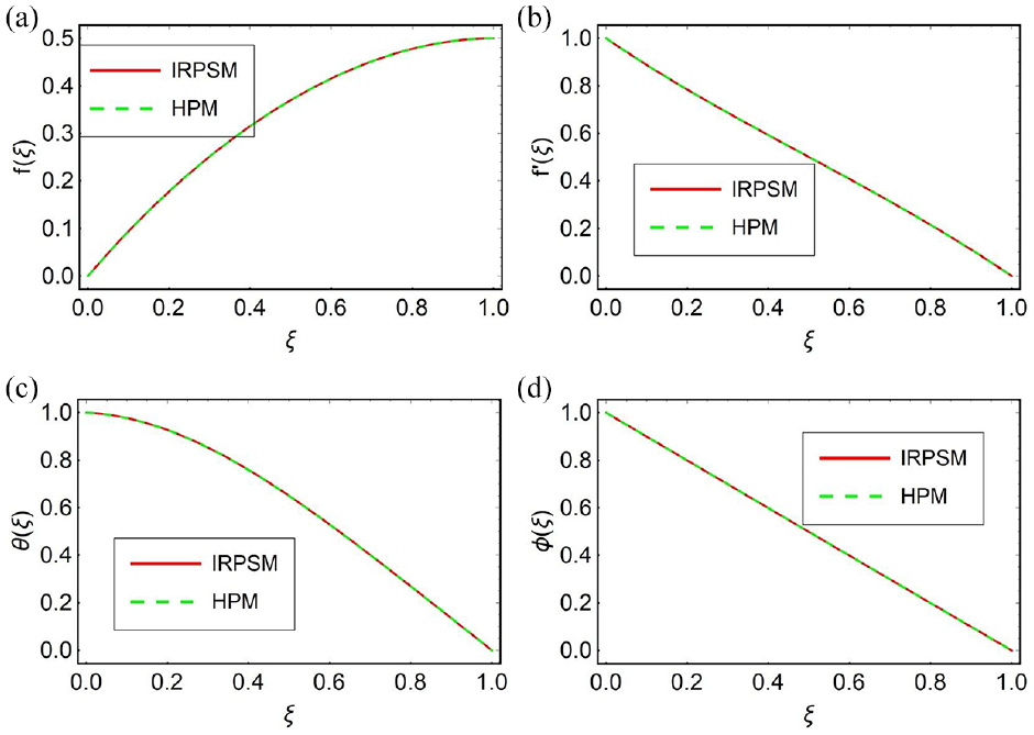
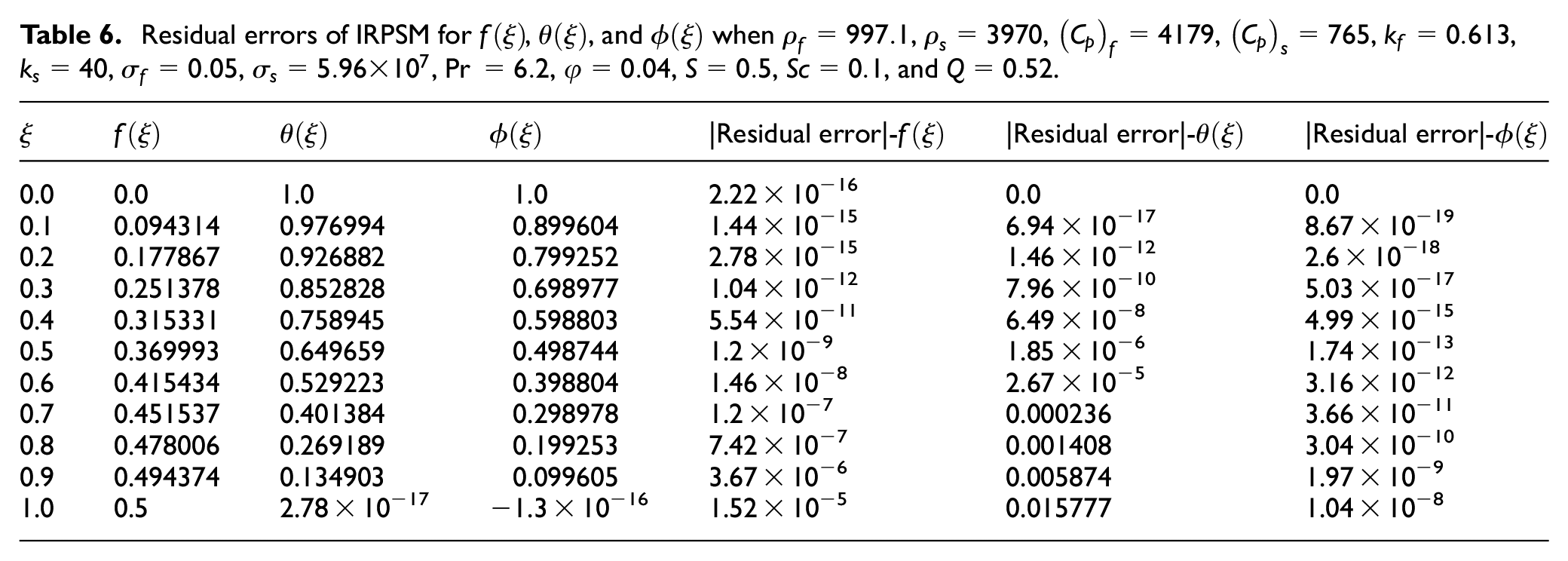
This section presents a comparison among the results obtained through numerical, IRPSM, and HPM techniques. A comparison of both analytical methods is determined at 17th order of approximations. Figure 2(a) to (d) are displayed to compare and verify both the methods for velocity, thermal, and concentration profiles when ${\rho }_f=997.1$ , ${\rho }_s=3970$ , ${\left(C_p\right)}_f=4179$ , ${\left(C_p\right)}_s=765$ , $k_f=0.613$ , $k_s=40$ , ${\sigma }_f=0.05$ , ${\sigma }_s=5.96\times 10^7$ , $\phi =0.04$ , $S=0.5$ , $\mathrm{Sc}=0.1$ , and $Q=0.52$ . From these Figures, it is seen that both the IRPSM and HPM are in great agreement and have a very close relation. Furthermore, Tables 2 to 5 are displayed to verify the results of all the three methods. From these Tables, it is seen that the absolute error between both the IRPSM and numerical methods, and HPM and numerical methods are very significant for solving such type of mathematical problems. Also, it has been found that the absolute error between the IRPSM and numerical method is more significant than the absolute error between the HPM and numerical method. This shows that IRPSM is stronger than HPM. Figure 3(a) to (c), and Tables 6 and 7 are displayed to study the residual of IRPSM and HPM for the velocity, temperature, and concentration profiles when ${\rho }_f=997.1$ , ${\rho }_s=3970$ , ${\left(C_p\right)}_f=4179$ , ${\left(C_p\right)}_s=765$ , $k_f=0.613$ , $k_s=40$ , ${\sigma }_f=0.05$ , ${\sigma }_s=5.96\times 10^7$ , $\phi =0.04$ , $S=0.5$ , $\mathrm{Sc}=0.1$ , and $Q=0.52$ . From here, it can see that the residuals of IRPSM are quite significant in term of less residual errors than that of HPM. Thus, it is confirmed that the IRPSM is more powerful method than the HPM in term of solving such type of mathematical problems.

Figure 2.

(a–d) Comparison of IRPSM and HPM for $f\left(\xi \right)$ , $f\prime \left(\xi \right)$ , $\theta \left(\xi \right)$ , and $\varphi \left(\xi \right)$ when ${\rho }_f=997.1$ , ${\rho }_s=3970$ , ${\left(C_p\right)}_f=4179$ , ${\left(C_p\right)}_s=765$ , $k_f=0.613$ , $k_s=40$ , ${\sigma }_f=0.05$ , ${\sigma }_s=5.96\times 10^7$ , $\mathrm{Pr}=6.2$ , $\phi =0.04$ , $S=0.5$ , $\mathrm{Sc}=0.1$ , and $Q=0.52$ .

Table 2.

Comparison of numerical, IRPSM, and HPM techniques for $f\left(\xi \right)$ when ${\rho }_f=997.1$ , ${\rho }_s=3970$ , ${\left(C_p\right)}_f=4179$ , ${\left(C_p\right)}_s=765$ , $k_f=0.613$ , $k_s=40$ , ${\sigma }_f=0.05$ , ${\sigma }_s=5.96\times 10^7$ , $\mathrm{Pr}=6.2$ , $\phi =0.04$ , $S=0.5$ , $\mathrm{Sc}=0.1$ , and $Q=0.52$ .

$\xi$	$f\left(\xi \right)$
	Numerical	IRPSM	HPM	|IRPSM-Numerical|	|HPM-Numerical|
0.0	0.0	0.0	0.0	0.0	0.0
0.1	0.094314435	0.094314440	0.094314441	5.438376082800289 × 10−9	5.655065540843829 × 10−9
0.2	0.177866916	0.177866921	0.177866924	4.733047370697463 × 10−9	7.632805804069775 × 10−9
0.3	0.251377810	0.251377814	0.251377823	3.680829530061658 × 10−9	1.281748951420525 × 10−8
0.4	0.315330507	0.315330509	0.315330527	2.552183131498964 × 10−9	1.9889790869864754 × 10−8
0.5	0.369992940	0.369992941	0.369992965	1.419649453548999 × 10−9	2.561280809665334 × 10−8
0.6	0.415434248	0.415434248	0.415434274	3.593031983051276 × 10−10	2.6765847205290072 × 10−8
0.7	0.451537123	0.451537122	0.451537145	6.779185546257338 × 10−10	2.178226232718572 × 10−8
0.8	0.478006308	0.478006306	0.478006320	1.6343567610377363 × 10−10	1.2073171740123456 × 10−8
0.9	0.494373643	0.494373640	0.494373645	2.435663615241168 × 10−10	1.8916354038722716 × 10−9
1.0	0.500000002	0.5	0.499999999	2.9360632813890675 × 10−10	2.9360633369002187 × 10−9

Table 3.

Comparison of numerical, IRPSM, and HPM techniques for $f\prime \left(\xi \right)$ when ${\rho }_f=997.1$ , ${\rho }_s=3970$ , ${\left(C_p\right)}_f=4179$ , ${\left(C_p\right)}_s=765$ , $k_f=0.613$ , $k_s=40$ , ${\sigma }_f=0.05$ , ${\sigma }_s=5.96\times 10^7$ , $\mathrm{Pr}=6.2$ , $\phi =0.04$ , $S=0.5$ , $\mathrm{Sc}=0.1$ , and $Q=0.52$ .

$\xi$	$f\prime \left(\xi \right)$
	Numerical	IRPSM	HPM	|IRPSM-Numerical|	|HPM-Numerical|
0.0	1.0	1.0	1.0	0.0	0.0
0.1	0.887923985	0.887923961	0.887923971	2.4054897296288402 × 10−8	1.367782420658159 × 10−8
0.2	0.784321787	0.784321777	0.784321822	1.0260297833575294 × 10−8	3.4886982747117656 × 10−8
0.3	0.686698175	0.686698163	0.686698240	1.2017469908087719 × 10−8	6.475135605477078 × 10−8
0.4	0.592799549	0.592799538	0.592799620	1.1212985762121264 × 10−8	7.021383940930548 × 10−8
0.5	0.500562288	0.500562277	0.500562326	1.0991628385248475 × 10−8	3.8885765163421127 × 10−8
0.6	0.408066955	0.408066944	0.408066936	1.0702497110770537 × 10−8	1.9034833487197034 × 10−8
0.7	0.313497623	0.313497613	0.313497545	1.0050415943929636 × 10−8	7.838485843736365 × 10−8
0.8	0.215105490	0.215105481	0.215105381	8.958474045916986 × 10−9	1.0848900433568787 × 10−7
0.9	0.111176149	0.111176142	0.111176064	7.138337212997392 × 10−9	8.532178738529517 × 10−8
1.0	2.0166 × 10−9	1.2675 × 10−16	6.9575 × 10−17	2.016163491372977 × 10−9	2.016163548554477 × 10−9

Table 4.

Comparison of numerical, IRPSM, and HPM techniques for $\theta \left(\xi \right)$ when ${\rho }_f=997.1$ , ${\rho }_s=3970$ , ${\left(C_p\right)}_f=4179$ , ${\left(C_p\right)}_s=765$ , $k_f=0.613$ , $k_s=40$ , ${\sigma }_f=0.05$ , ${\sigma }_s=5.96\times 10^7$ , $\mathrm{Pr}=6.2$ , $\phi =0.04$ , $S=0.5$ , $\mathrm{Sc}=0.1$ , and $Q=0.52$ .

$\xi$	$\theta \left(\xi \right)$
	Numerical	IRPSM	HPM	|IRPSM-Numerical|	|HPM-Numerical|
0.0	1.0	1.0	1.0	0.0	0.0
0.1	0.977013227	0.976993805	0.976699123	0.000019422699891968875	0.0003141045945168619
0.2	0.926919838	0.926881977	0.926349111	0.00003786054906940173	0.0005707267689470941
0.3	0.852882669	0.852828197	0.852146833	0.00005447268216007828	0.0007358362675806696
0.4	0.759013332	0.758944662	0.758212200	0.00006866971285568457	0.0008011318830656311
0.5	0.649738909	0.649658821	0.648962003	0.00008008765882017155	0.0007769061356327489
0.6	0.529311895	0.529223370	0.528628922	0.00008852453192620402	0.000682973173172341
0.7	0.401477858	0.401384220	0.400936567	0.00009363719209759536	0.0005412908034971298
0.8	0.269281888	0.269188716	0.268910570	0.00009317221883436977	0.0003713183356869876
0.9	0.134978035	0.134790653	0.134790246	0.00007549496769715391	0.0001877896946593515
1.0	1.1296 × 10−8	−1.0061 × 10−16	−1.0061 × 10−16	1.129697783447863 × 10−8	1.12969779628467 × 10−8

Table 5.

Comparison of numerical, IRPSM, and HPM techniques for $\varphi \left(\xi \right)$ when ${\rho }_f=997.1$ , ${\rho }_s=3970$ , ${\left(C_p\right)}_f=4179$ , ${\left(C_p\right)}_s=765$ , $k_f=0.613$ , $k_s=40$ , ${\sigma }_f=0.05$ , ${\sigma }_s=5.96\times 10^7$ , $\mathrm{Pr}=6.2$ , $\phi =0.04$ , $S=0.5$ , $\mathrm{Sc}=0.1$ , and $Q=0.52$ .

$\xi$	$\varphi \left(\xi \right)$
	Numerical	IRPSM	HPM	|IRPSM-Numerical|	|HPM-Numerical|
0.0	1.0	1.0	1.0	0.0	0.0
0.1	0.899604291	0.899604291	0.899604292	2.939015697478453 × 10−11	1.3400202059088429 × 10−9
0.2	0.799252162	0.799252162	0.799252165	2.1723067789025663 × 10−8	2.6327210411736246 × 10−9
0.3	0.698977304	0.698977304	0.698977308	1.1000977906405751 × 10−8	3.838023232560772 × 10−9
0.4	0.598803252	0.598803252	0.598803257	2.7106095146223197 × 10−12	4.809796450011561 × 10−9
0.5	0.498743890	0.498743890	0.498743896	2.330025061780816 × 10−12	5.354922838485265 × 10−9
0.6	0.398803754	0.398803754	0.398803759	4.954647803145917 × 10−12	5.308896489086834 × 10−9
0.7	0.298978140	0.298978140	0.298978145	2.939015697478453 × 10−11	4.613362580840885 × 10−9
0.8	0.199253037	0.199253037	0.199253040	2.1723067789025663 × 10−11	3.3585279002323887 × 10−9
0.9	0.099604859	0.099604859	0.099604861	1.1000977906405751 × 10−11	1.752182510195155 × 10−9
1.0	1.4282 × 10−11	−1.1680 × 10−16	−1.16801 × 10−16	2.7106095146223197 × 10−12	1.4282321590320099 × 10−11

Figure 3.

(a–c) Residual error of IRPSM and HPM for $f\left(\xi \right)$ , $\theta \left(\xi \right)$ , and $\varphi \left(\xi \right)$ when ${\rho }_f=997.1$ , ${\rho }_s=3970$ , ${\left(C_p\right)}_f=4179$ , ${\left(C_p\right)}_s=765$ , $k_f=0.613$ , $k_s=40$ , ${\sigma }_f=0.05$ , ${\sigma }_s=5.96\times 10^7$ , $\mathrm{Pr}=6.2$ , $\phi =0.04$ , $S=0.5$ , $\mathrm{Sc}=0.1$ , and $Q=0.52$ .

Table 6.

Residual errors of IRPSM for $f\left(\xi \right)$ , $\theta \left(\xi \right)$ , and $\varphi \left(\xi \right)$ when ${\rho }_f=997.1$ , ${\rho }_s=3970$ , ${\left(C_p\right)}_f=4179$ , ${\left(C_p\right)}_s=765$ , $k_f=0.613$ , $k_s=40$ , ${\sigma }_f=0.05$ , ${\sigma }_s=5.96\times 10^7$ , $\mathrm{Pr}=6.2$ , $\phi =0.04$ , $S=0.5$ , $\mathrm{Sc}=0.1$ , and $Q=0.52$ .

$\xi$	$f\left(\xi \right)$	$\theta \left(\xi \right)$	$\varphi \left(\xi \right)$	|Residual error|- $f\left(\xi \right)$	|Residual error|- $\theta \left(\xi \right)$	|Residual error|- $\varphi \left(\xi \right)$
0.0	0.0	1.0	1.0	2.22 × 10−16	0.0	0.0
0.1	0.094314	0.976994	0.899604	1.44 × 10−15	6.94 × 10−17	8.67 × 10−19
0.2	0.177867	0.926882	0.799252	2.78 × 10−15	1.46 × 10−12	2.6 × 10−18
0.3	0.251378	0.852828	0.698977	1.04 × 10−12	7.96 × 10−10	5.03 × 10−17
0.4	0.315331	0.758945	0.598803	5.54 × 10−11	6.49 × 10−8	4.99 × 10−15
0.5	0.369993	0.649659	0.498744	1.2 × 10−9	1.85 × 10−6	1.74 × 10−13
0.6	0.415434	0.529223	0.398804	1.46 × 10−8	2.67 × 10−5	3.16 × 10−12
0.7	0.451537	0.401384	0.298978	1.2 × 10−7	0.000236	3.66 × 10−11
0.8	0.478006	0.269189	0.199253	7.42 × 10−7	0.001408	3.04 × 10−10
0.9	0.494374	0.134903	0.099605	3.67 × 10−6	0.005874	1.97 × 10−9
1.0	0.5	2.78 × 10−17	−1.3 × 10−16	1.52 × 10−5	0.015777	1.04 × 10−8

Table 7.

Residual errors of HPM for $f\left(\xi \right)$ , $\theta \left(\xi \right)$ , and $\varphi \left(\xi \right)$ when ${\rho }_f=997.1$ , ${\rho }_s=3970$ , ${\left(C_p\right)}_f=4179$ , ${\left(C_p\right)}_s=765$ , $k_f=0.613$ , $k_s=40$ , ${\sigma }_f=0.05$ , ${\sigma }_s=5.96\times 10^7$ , $\mathrm{Pr}=6.2$ , $\phi =0.04$ , $S=0.5$ , $\mathrm{Sc}=0.1$ , and $Q=0.52$ .

$\xi$	$f\left(\xi \right)$	$\theta \left(\xi \right)$	$\varphi \left(\xi \right)$	|Residual error|- $f\left(\xi \right)$	|Residual error|- $\theta \left(\xi \right)$	|Residual error|- $\varphi \left(\xi \right)$
0.0	0.0	1.0	1.0	9.35 × 10−6	0.0	0.0
0.1	0.094314	0.976699	0.899604	2.62 × 10−5	0.004918	4.02 × 10−10
0.2	0.177867	0.926349	0.799252	2.96 × 10−5	0.007699	7.92 × 10−9
0.3	0.251378	0.852147	0.698977	1.9 × 10−5	0.008337	2.4 × 10−8
0.4	0.315331	0.758212	0.598803	6.05 × 10−9	0.007466	4.49 × 10−8
0.5	0.369993	0.648962	0.498744	1.95 × 10−5	0.00583	6.27 × 10−8
0.6	0.415434	0.528629	0.398804	3.16 × 10−5	0.004014	6.89 × 10−8
0.7	0.451537	0.400937	0.298978	3.14 × 10−5	0.002387	5.93 × 10−8
0.8	0.478006	0.268911	0.199253	1.8 × 10−5	0.001136	3.68 × 10−8
0.9	0.494374	0.13479	0.099605	5.28 × 10−6	0.000331	1.23 × 10−8
1.0	0.5	−1 × 10−16	−1.2 × 10−16	3.2 × 10−5	5.09 × 10−17	1.18 × 10−17

Results and discussion

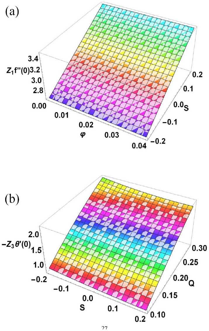
Figure 4(a) to (c) show the impact of $S$ on $f\left(\xi \right)$ , $f\prime \left(\xi \right)$ , and $\theta \left(\xi \right)$ when ${\rho }_f=997.1$ , ${\rho }_s=3970$ , ${\left(C_p\right)}_f=4179$ , ${\left(C_p\right)}_s=765$ , $k_f=0.613$ , $k_s=40$ , ${\sigma }_f=0.05$ , ${\sigma }_s=5.96\times 10^7$ , $\mathrm{Pr}=6.2$ , $\phi =0.04$ , $\mathrm{Sc}=0.1$ , and $Q=0.52$ . From Figure 4(a), it is observed that the higher values of $S$ increases $f\left(\xi \right)$ . From the given boundary conditions, it is seen that $S$ is a boundary parameter and has direct relation with $f\left(\xi \right)$ . This means that the higher values of $S$ increases $f\left(\xi \right)$ . From Figure 4(b), it is observed that the higher values of $S$ increases $f\prime \left(\xi \right)$ . From here it is see that the greater values of $S$ increases $f\prime \left(\xi \right)$ both positive and negative values of $S$ . A similar impact is also found by Acharya et al. ¹⁶ From Figure 4(c), it is observe that the positive values of $S$ reduce $\theta \left(\xi \right)$ while the negative values of $S$ increases $\theta \left(\xi \right)$ . Physically, the negative values of $S$ means that the plates become closer and as a result less fraction between the nanoparticles and plates occurs. Therefore, the temperature profile reduces for negative values of $S$ . On the other hand, this impact is reverse for positive values of $S$ . Figure 5 shows the impact of $Q$ on $\theta \left(\xi \right)$ when ${\rho }_f=997.1$ , ${\rho }_s=3970$ , ${\left(C_p\right)}_f=4179$ , ${\left(C_p\right)}_s=765$ , $k_f=0.613$ , $k_s=40$ , ${\sigma }_f=0.05$ , ${\sigma }_s=5.96\times 10^7$ , $\mathrm{Pr}=6.2$ , $\phi =0.04$ , $\mathrm{Sc}=0.1$ , and $S=0.5$ . From this Figure, it is observed that the greater $Q$ increases $\theta \left(\xi \right)$ . The reason is that the increase in $Q$ increases the rate of heat transfer which results higher thermal profile. Therefore, the greater $Q$ increases $\theta \left(\xi \right)$ . Figure 6 show the impact of $\mathrm{Sc}$ on $\varphi \left(\xi \right)$ when ${\rho }_f=997.1$ , ${\rho }_s=3970$ , ${\left(C_p\right)}_f=4179$ , ${\left(C_p\right)}_s=765$ , $k_f=0.613$ , $k_s=40$ , ${\sigma }_f=0.05$ , ${\sigma }_s=5.96\times 10^7$ , $\mathrm{Pr}=6.2$ , $\phi =0.04$ , $S=0.5$ , and $Q=0.52$ . From this Figure, it is observed that the greater $\mathrm{Sc}$ reduces $\varphi \left(\xi \right)$ . The higher $\mathrm{Sc}$ reduces the Brownian diffusivity which results lower $\varphi \left(\xi \right)$ . Therefore, the higher $\mathrm{Sc}$ reduces $\varphi \left(\xi \right)$ . Figure 7(a) shows the variation in $-Z_{1}f″\left(0\right)$ for $\phi$ and $S$ . Here, $\phi$ and $S$ are varied for different values and all other parameters are taken constant. From here, it is perceived that the greater values of $\phi$ and $S$ increases the friction force at the surface of the plate. Figure 7(b) shows the variation in $-Z_3\theta \prime \left(0\right)$ for $\phi$ and $Q$ . Here, $\phi$ and $Q$ are varied for different values and all other parameters are taken constant. From here, it is perceived that the greater values of $\phi$ and $Q$ increases the heat transfer rate at the surface of the plate. Table 8 is displayed to observe the numerical results of $-Z_{1}f″\left(0\right)$ and $-Z_3\theta \prime \left(0\right)$ for the increasing $S$ when ${\rho }_f=997.1$ , ${\rho }_s=3970$ , ${\left(C_p\right)}_f=4179$ , ${\left(C_p\right)}_s=765$ , $k_f=0.613$ , $k_s=40$ , ${\sigma }_f=0.05$ , ${\sigma }_s=5.96\times 10^7$ , $\mathrm{Pr}=6.2$ , $\phi =0.04$ , $\mathrm{Sc}=0.1$ , and $Q=0.52$ . Here, both the IRPSM and HPM methods are tested for different values of $S$ . Again, it is confirmed that both the IRPSM and HPM are applicable for solving such type of mathematical problems.

Figure 4.

(a–c) Impact of $S$ on $f\left(\xi \right)$ , $f\prime \left(\xi \right)$ , and $\theta \left(\xi \right)$ when ${\rho }_f=997.1$ , ${\rho }_s=3970$ , ${\left(C_p\right)}_f=4179$ , ${\left(C_p\right)}_s=765$ , $k_f=0.613$ , $k_s=40$ , ${\sigma }_f=0.05$ , ${\sigma }_s=5.96\times 10^7$ , $\mathrm{Pr}=6.2$ , $\phi =0.04$ , $\mathrm{Sc}=0.1$ , and $Q=0.52$ .

Figure 5.

Impact of $Q$ on $\theta \left(\xi \right)$ when ${\rho }_f=997.1$ , ${\rho }_s=3970$ , ${\left(C_p\right)}_f=4179$ , ${\left(C_p\right)}_s=765$ , $k_f=0.613$ , $k_s=40$ , ${\sigma }_f=0.05$ , ${\sigma }_s=5.96\times 10^7$ , $\mathrm{Pr}=6.2$ , $\phi =0.04$ , $S=0.5$ , and $\mathrm{Sc}=0.1$ .

Figure 6.

Impact of $\mathrm{Sc}$ on $\varphi \left(\xi \right)$ when ${\rho }_f=997.1$ , ${\rho }_s=3970$ , ${\left(C_p\right)}_f=4179$ , ${\left(C_p\right)}_s=765$ , $k_f=0.613$ , $k_s=40$ , ${\sigma }_f=0.05$ , ${\sigma }_s=5.96\times 10^7$ , $\mathrm{Pr}=6.2$ , $\phi =0.04$ , $S=0.5$ , and $Q=0.52$ .

Figure 7.

(a and b) Variations in $Z_{1}f″\left(0\right)$ and $-Z_3\theta \prime \left(0\right)$ when ${\rho }_f=997.1$ , ${\rho }_s=3970$ , ${\left(C_p\right)}_f=4179$ , ${\left(C_p\right)}_s=765$ , $k_f=0.613$ , $k_s=40$ , ${\sigma }_f=0.05$ , ${\sigma }_s=5.96\times 10^7$ , $\mathrm{Pr}=6.2$ , $S=0.5$ , $\phi =0.04$ , $\mathrm{Sc}=0.1$ , and $Q=0.52$ .

Table 8.

Numerical values of $Z_{1}f″\left(0\right)$ and $-Z_3\theta \prime \left(0\right)$ for the increasing $S$ when ${\rho }_f=997.1$ , ${\rho }_s=3970$ , ${\left(C_p\right)}_f=4179$ , ${\left(C_p\right)}_s=765$ , $k_f=0.613$ , $k_s=40$ , ${\sigma }_f=0.05$ , ${\sigma }_s=5.96\times 10^7$ , $\mathrm{Pr}=6.2$ , $\phi =0.04$ , $\mathrm{Sc}=0.1$ , and $Q=0.52$ .

$S$	HPM		IRPSM
	$Z_{1}f″\left(0\right)$	$-Z_3\theta \prime \left(0\right)$	$Z_{1}f″\left(0\right)$	$-Z_3\theta \prime \left(0\right)$
−0.2	−5.1999318	1.0944531	−5.1992456	1.0953475
−0.1	−4.6470133	0.8623464	−4.6474535	0.8635774
0.1	−3.5183300	0.6840077	−3.5154343	0.6850865
0.2	−2.9427700	0.5509772	−2.9453245	0.5515335

Conclusions and future scope

In this paper the squeezing flow problem between two parallel plates has been investigated successfully. The nanofluid flow comprising alumina (Al₂O₃) nanoparticles and water is used as a base fluid. A comparative analysis among the numerical, IRPMS, and HPM techniques has been successfully presented in this effort. The comparison of both IRPSM and HPM is conducted at 17th order of approximations. From this analysis, it is concluded that:

• • The numerical, IRPSM, and HPM techniques are in great agreement and have a very close relation.

• • The results of both methods are compared with the numerical method and found that the absolute error between both the IRPSM and numerical techniques, and HPM and numerical techniques are very significant for solving such type of mathematical problems.

• • It is seen that the residuals of IRPSM are quite significant in term of less residual errors then those of HPM.

• • It is confirmed that the IRPSM is more powerful method than the HPM in term of solving such type of mathematical problems.

Future recommendations

In future, the IRPSM can be implemented to slip flow of nanofluids in a two rotating disk and parallel plates. Furthermore, the convective and mass flux conditions can also be imposed in a nanofluid flow to determine the series solutions via IRPSM. Also, the IRPSM can also be compared with other analytical and numerical methods to check effectiveness of IRPSM.