Fluctuating pressure gradients and corrugated surfaces effects on wind turbines power output

Abstract

This paper investigates the effect of corrugated surfaces on the wind turbines power output for both laminar and turbulent flows. Conservation principles including continuity and momentum equations, wind turbine power equations, and the corrugated surface equation have been implemented to build up a theoretical model then which has been solved using MATLAB. This model simulates wind turbines power output and analyzes several case studies implementing different parameters such as air pressure wave amplitude (P_o), air wave fluctuation frequency (n), and wind layer turbulence (b). Also, different complex terrains in two main scenarios representing two different positions (X) of the wind turbine are analyzed. This analysis indicates the importance of wind turbines micro siting. In addition, it is found that increasing the pressure ratio increased wind turbine power output, while increasing the frequency decreased the power ratio of the wind turbines for both laminar and turbulent flow conditions. Increasing turbulence for the turbulent model increased the power ratio.

Introduction

Renewable energy has become one of the most important topics of interest in the world, as fossil fuels are depleting and their usage negatively impact environment, health, and overall wellbeing. Wind energy is a renewable energy resource advancing rapidly among other renewable energies, as the total installed wind capacity reached 906 GW in 2022. Wind is a natural occurrence that could be defined as the flow of gases on a large scale. It is considered a renewable energy resource, which is sustainable, unlimited, free, and environmentally friendly, as it does not emit greenhouse gases or air pollutants. The first electricity-generating wind turbine was invented in 1888 by Charles F. Brush in Cleveland, Ohio. The turbine’s diameter was 17 m, it had 144 rotor blades made of cedar wood, and it generated around 12 kW of power. Today, the biggest commercial wind turbine in the world has hit a capacity of 9.5 MW and a rotor diameter of 164 m. However, the working principle has remained the same. Wind turbines transform the kinetic energy of the wind into electrical energy. The wind, which is essentially moving air, pushes against the blades of the turbine, making them rotate. In the process, some of the kinetic energy of the moving air is transformed into the mechanical (rotational kinetic) energy of the spinning blades. According to Betz law, no turbine can capture more than 16/27 (59.3%) of the kinetic energy in the wind. The factor 16/27 (0.593) is known as Betz’s coefficient. So theoretically speaking, a wind turbine is able to extract 59.3% of wind’s kinetic energy, however real utility-scale wind turbines achieve at peak 75%–80% of the Betz limit. Furthermore, there are several other factors limiting the useful power output from wind farms such as air turbulence and complex terrains effects. The turbulence (or gusts) could be defined as the wind variation above earth’s surface in an indefinite pattern and strength. It causes random, fluctuating loads and stresses over the whole turbine structure, resulting into power fluctuations hence the fatigue of the wind turbine. Complex terrains are defined by the International Electrotechnical Commission Standard IEC 61400 as being those with inclination over 10°. Complex terrains can also include variations in land use, such as urban, rural, irrigated, and unirrigated that cause flow distortion.

Air turbulence plays a very important role in the energy produced by wind turbines. A lot of research has been done and numerous papers have been published where the impact of wind turbulence on the final output of wind turbines is analyzed and discussed. Rohatgi and Barbezier ¹ analyzed the effect of wind turbulence on the output of large-sized wind turbines and explained that turbulence causes random, fluctuating loads and stresses over the whole structure, resulting into power fluctuations hence the fatigue of the wind turbine. They stated that an unstable atmosphere is more advantageous for wind power generation because of higher wind speeds, whereas a stable atmosphere is worse because it suffers from both the increased shear over the rotor diameter, as well as the reduced wind speed.

Marimuthu and Kirubakaran ² tested wind speed, turbine swept area, and air density on two different turbines models; V1.65MW and V1.8MW and concluded that the maximum output is obtained at the maximum wind speed and it is directly proportional to the air density, so the selection of wind turbines should be based on the geographical features and the climate condition of the particular site. Ozbay ³ conducted several experiments on wind turbines and one of the main conclusions of the experiment was that higher levels of turbulence in the oncoming flow, as in the onshore case, caused greater fluctuations in the rotational speed of the wind turbine. They also caused fluctuations in the wind loads acting on the wind turbine, which could impose higher dynamic loads on the wind turbine components. Stival ⁴ analyzed wind data collected using LiDAR and SCADA from a North American Wind Farm. They stated that when low turbulence intensity develops in conjunction with high values of wind shear, the power production might be significantly affected.

Vahidzadeh and Markfort ⁵ pointed out that prediction of wind turbines energy production using power curves is not very accurate because power curves are based on ideal uniform inflow wind, which is not the case in complex and heterogeneous terrains. They proposed a new prediction mathematical model and compared the resulting power curve with real data power curve from a 2.5 MW wind turbine. The comparison results showed the proposed models performed better than the standard power curve, reducing power prediction error as much as 75%. They also concluded that – generally stated – all models over-predict power generation when turbulence intensity is low and under-predict it at high turbulence intensity levels. Hence the effect of turbulence intensity is an important aspect which needs to be further investigated. Anup et al. ⁶ analyzed data from a flat terrain site in Östergarnsholm (OG) and from built environment site at Port Kennedy (PK) using the aeroelastic code FAST (Fatigue, Aerodynamics, Structures, and Turbulence). Then they compared the obtained data with IEC 61400-2. The longitudinal turbulence intensity (TIu) in the PK wind field was 22%; which was higher than the estimated value in IEC 61400-2 Normal Turbulence Model. The elevated turbulence in PK wind fields increased the output rotor power which was higher than that stipulated in the standard. They concluded that the current IEC standard isn’t very accurate for urban siting of small wind turbines hence needs further amendments for more reliable implementation in turbulent sites.

Wu et al. ⁷ executed a series of large-eddy simulations (LESs) to study the impact of different incoming turbulent boundary layer flows on large wind farms. They used four incoming flow conditions from the LESs of the Atmospheric Boundary Layer flow over homogeneous flat surfaces with four different aerodynamic roughness lengths (z = 0.5, 0.1, 0.01, and 0.0001 m), where the hub-height turbulence intensity levels were around 11.1%, 8.9%, 6.8%, and 4.9%, respectively.

Based on the simulation results they concluded that an improvement in the inflow turbulence level can increase the power generation efficiency in large wind farms; 23.3% increment on the overall farm power production and around 32.0% increment on the downstream turbine power production.

Ismaiel ⁸ investigated the dynamics of a wind turbine’s blade under the effect of atmospheric turbulence. He simulated the WindPact 1.5 MW turbine under different turbulent wind fields, all having a mean wind velocity of 12 m/s but with turbulence intensities of 1%, 10%, 25%, and 50%. He observed that the higher the turbulence intensity, the severer the fluctuations of the deflection around its mean value. He recommended to put the turbine immediately on brake in case of gusts or severe turbulence exceeding a certain limit, based on the turbine design. He also suggested forecasts be made ahead of turbine installation in a wind farm. If the chance of gusts occurring is high, then a downwind turbine could be safer and allow higher deflections avoiding tower strikes danger. At the end, he pointed out the importance of continuous monitoring of the atmospheric turbulence in a wind farm.

Cai et al. ⁹ executed wind-tunnel experiments to study the effect of favorable and adverse constant pressure gradients (PG) caused by local changes in the topography just downwind of a model wind turbine. They used particle image velocimetry to characterize the near and intermediate wake regions. They studied five scenarios, two favorable PG, two adverse PG, and a scenario with negligible PG. The results they obtained showed that the PGs induce a wake deflection and modulate the wake. Pressure Gradients imposed a relatively small impact on the kinematic shear stress and the turbulence kinetic energy; however, they have a comparatively dominant effect on the bulk flow on the flow recovery.

The research done in the field of corrugated surfaces impact on the wind turbines power output is little. Until today, no exact specific equations have been found to express how the geometry of complex topography influences the final output power of turbines. Botta et al. ¹⁰ have examined the wind turbines performance at Acqua Spruza; a mountainous test site located in the Apennine Mountains in Italy, at an average altitude of 1350, which is characterized by harsh weather conditions such as high turbulence, high vertical component of wind velocity, snowfalls, and heavy icing. After taking several power measurements, they concluded that complex terrains directly influence both the energy output and the steady and fatigue loading of wind turbines. Therefore, the construction of wind turbines in mountainous areas should be managed with high awareness. Elgendi et al. ¹¹ conducted a comprehensive review of wind turbines in complex terrain. They concluded that the exact positioning of turbines is critical for wind locations with significant topographical change, as the flow accelerations and retardations produced by local topography characteristics could disrupt the wake of wind turbines constructed in hilly regions. In addition, they stated that the distance between consecutive turbines in the wind farm should be precisely calculated to trade-off between wind farm cost and wind turbine performance. Ayala et al. ¹² have investigated a 16.5 MW wind farm located in a complex terrain in the Ecuadorian Andes at an elevation of 2700 m a.s.l. After comparing between the actual power production data with the expected power production data predicted by Meteodyn WT software – a CFD tool based on a nonlinear flow model – they found a power underestimation of around 12.47%. These results clearly show that simulation software programs still have inaccuracies and need more validation. Kwon ¹³ has evaluated the wind resource of a wind turbine using uncertainty analysis. In his study he mentioned that the surface roughness (which is a type of natural phenomena) at a specific site, is dependent on the terrain condition, and varies from 0.128 to 0.160 even in a very homogeneous surface such as flat or farm land. As a consequence, the uncertainty of wind velocity according to height is caused by the ambiguity of surface roughness at the site. Tabas et al. ¹⁴ have simulated the wind field and wind farm power output in Juvent Wind Farm located in the complex terrain of Swiss Jura Mountains using WindSim software. The distinct feature of this site is that it hosts three different complexities; topography, heterogeneous vegetation with a woodland-grassland mosaic, and interactions between wind turbine wakes. They concluded that simulation results were sensitive to the choice of modeling schemes and parameters. Hence, more validations at different sites of complex terrain are needed before any model. In addition, high-resolution terrain and vegetation data such as canopy density and height are needed to precisely estimate the relevant parameters for numerical wind energy prediction in the case of forested mountainous regions.

Zhao et al. ¹⁵ have studied the wake development characteristics of wind farms in complex terrains. They took the measurements of a mountainous area in Hebei Province, China using two different types of LiDAR devices. They concluded that the wind speed gradually increases above the wake center and wake recovery rate is determined by both the incoming wind turbulence intensity in the wake and the magnitude of the wind speed. Based on the results, they recommended the use of specific pitch/yaw control strategies for specific turbines in order to improve the aerodynamic performance of the downwind wind turbines. Liu and Stevens ¹⁶ performed large eddy simulations for different atmospheric conditions to examine the impact of a three-dimensional hill on the performance of a downwind turbine. They made the distance between the hill and the turbine six times the turbine diameter, and the hill height equal to the hub height. Their simulations showed that the hill wake reduced the power production of the downstream turbine by 35% for the convective boundary layer case under consideration. On the other hand, the wind turbine power production increased by around 24% for the stable boundary layer case considered in the study. This phenomenon resulted from the entrainment of kinetic energy from the low-level jet due to the increased mixing induced by the hill wake.

In this study, the effects of fluctuating pressure gradients and corrugated surfaces (complex terrains) on the output of a selected wind turbine model are studied. A theoretical model is built up by using continuity, transient momentum, and wind turbine equations, in addition to the corrugated surface equation for the estimation of power output for both laminar and turbulent flow conditions, in order to study the effect of air steam fluctuations on the wind turbine power output. These equations are solved using the MATLAB program for different scenarios and the resultant simulations are analyzed. The impact of fluctuating pressure gradients on wind turbines output is analyzed in several case studies implementing three parameters which are air wave amplitude (P_o), air wave fluctuation frequency (n), and air turbulence (b). To analyze the effect of complex terrains, different case studies including the above-mentioned parameters are analyzed in two scenarios which represent different positions (X) of the wind turbine.

Mathematical modeling and solutions

The Navier-Stokes equations express the motion of viscous fluids and in this case are transformed to capture earth topography effects on turbine power output, under the assumptions of transient two-dimensional incompressible flow and neglecting body forces. This study implemented analytical (theoretical) solutions for different variables (P_o, n, b) for both cases of laminar and turbulent flows. The physical model and coordinate systems are shown in Figure 1.

Figure 1.

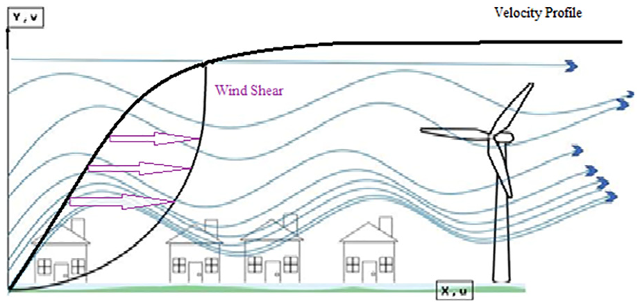
Physical model and coordinates system.

The wind flow against wind turbine is formulated according to three fundamental laws of physics: conservation of mass, conservation of momentum side by side with topography equations, and wind turbine power output equations. ¹⁷ These principles can be expressed as:

$$\frac{\partial \mathrm{u}}{\partial \mathrm{x}}+\frac{\partial \mathrm{v}}{\partial \mathrm{y}}=0$$

(1)

The x-Momentum equation suitable for wind turbine dynamics is shown below and according to boundary layer approximations the y-Momentum equation is neglected because of its small order of magnitude.

$$\frac{\partial \mathrm{u}}{\partial \mathrm{t}}+\mathrm{u}\frac{\partial \mathrm{u}}{\partial \mathrm{x}}+\mathrm{v}\frac{\partial \mathrm{u}}{\partial \mathrm{y}}=-\frac{1}{\mathrm{\rho }}\frac{\partial \mathrm{P}}{\partial \mathrm{x}}+v*\mathrm{b}(\frac{{\partial }^{2}u}{\partial x^2}+\frac{{\partial }^{2}u}{\partial y^2})$$

(2)

In equation (2) the nonlinear terms (first order derivatives) are neglected assuming parallel flow in the direction of the wind turbine (v = 0) and also the second order derivative with respect to x, because of the small order of magnitude, simplifying the equation to equation (3) shown below:

$$\frac{\partial \mathrm{u}}{\partial \mathrm{t}}=-\frac{1}{\mathrm{\rho }}\frac{\partial \mathrm{P}}{\partial \mathrm{x}}+v*\mathrm{b}\left(\frac{{\partial }^{2}u}{\partial y^2}\right)$$

(3)

In the above equations u is the velocity component on the x-axis (axial velocity), v is the velocity component on the y-axis, t: is the Time (s), p is the air pressure (Pa), υ: is the kinematic viscosity (m²/s) which is equal to (v = μ/ ρ), μ: is the dynamic viscosity (Pa × s) and ρ is the air density (kg/m³). b is the air turbulence level and is equal to (b = 1 +  ${\epsilon }_{\mathrm{m}}^{+}$ ), where ${\epsilon }_{\mathrm{m}}^{+}$ is the dimensionless eddy viscosity defined by ( ${\epsilon }_{\mathrm{m}}^{+}$  = ε_m/ν).

Hilly terrains and mountainous areas are among the best complex terrains for wind farms construction. The most appropriate representation of these complex terrains is the sinusoidal shape. Therefore, the corrugated surface equation has been represented by the sinusoidal waveform given by equation (4):

$$\sigma (\mathrm{x})=\mathrm{asin}\left(\frac{2\mathrm{\pi }\mathrm{x}}{\lambda }\right)$$

(4)

Here σ is the corrugated surface equation, where a is the amplitude of the sinusoidal wave and $\lambda$ is the wavelength of the curve and x is the position of the wind turbine on the sinusoidal waveform. In order to incorporate the topography effects on the governing equations the following set of transformations are used and shown in Figure 2:

$$\mathrm{x}*=\mathrm{x};\mathrm{y}*=\mathrm{y}-\sigma (\mathrm{x})$$

(5)

Figure 2.

Corrugated surface function representation.

After substituting equation (5) in equation (3) the following equation is obtained:

$$\frac{\partial \mathrm{u}}{\partial \mathrm{t}}=-\int \frac{1}{\mathrm{\rho }}\frac{\partial \mathrm{P}}{\partial \mathrm{x}}+\nu (1+\sigma (\mathrm{x}))\frac{\partial }{\partial \mathrm{y}}\left(\mathrm{b}\frac{\partial \mathrm{u}}{\partial \mathrm{y}}\right)$$

(6)

This is a second partial differential equation and none homogeneous. The air waves are usually modeled as sinusoidal wave forms. This is because actual data of wind speeds show that air blows at speeds which repeat themselves cyclically during a specific period of time. So, the fluctuating pressure gradient of air wave is assumed to be a sinusoidal wave, as can be seen in equation (7):

$$-\frac{1}{\mathrm{\rho }}\frac{\partial p}{\partial x}=p_0\cos (\mathrm{nt})$$

(7)

Here, p_o refers to the air wave fluctuation amplitude (m/s²) and n refers to the fluctuation cycle number (cycle/h). The corresponding initial and boundary conditions are:

$$\begin{array}{c}t=0\mathrm{for}\mathrm{all}\mathrm{y}u(0,x,y)=0\hfill \\ t>0\mathrm{y}=0u(t,x,0)=0\hfill \\ t>0y\to \infty u(t,x,\infty )=u_{\infty }\hfill \end{array}$$

(8)

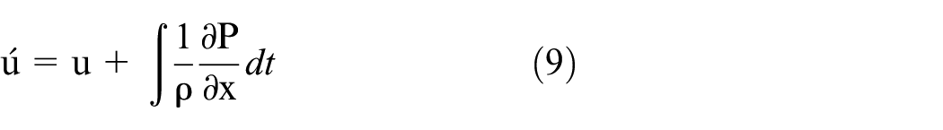
The following assumption has been made; ú is a new variable has been defined as the summation of the velocity and the integration of the fluctuating pressure gradients of the wind as shown in equation (9) in order to make the governing equation a homogeneous ordinary differential equation:

$$\stackrel{\prime }{\mathrm{u}}=\mathrm{u}+\int \frac{1}{\mathrm{\rho }}\frac{\partial \mathrm{P}}{\partial \mathrm{x}}\mathrm{dt}$$

(9)

Substituting equation (9) into equation (6), the following governing momentum equation is obtained:

$$\frac{\partial \stackrel{\prime }{\mathrm{u}}}{\partial \mathrm{t}}=\mathrm{\nu }(1+\sigma (\mathrm{x}))\frac{\partial }{\partial \mathrm{y}}\left(\mathrm{b}\frac{\partial \stackrel{\prime }{\mathrm{u}}}{\partial \mathrm{y}}\right)$$

(10)

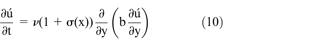
Now the following non-dimensional variables are adopted to rewrite the governing equation in a proper non-dimensional form:

$$u^{*}=\frac{\stackrel{\prime }{\mathrm{u}}}{u_{\infty }}{y}^{*}=\frac{y{u}_{\infty }}{v}{\mathrm{t}}^{*}=\frac{t}{t_o}$$

(11)

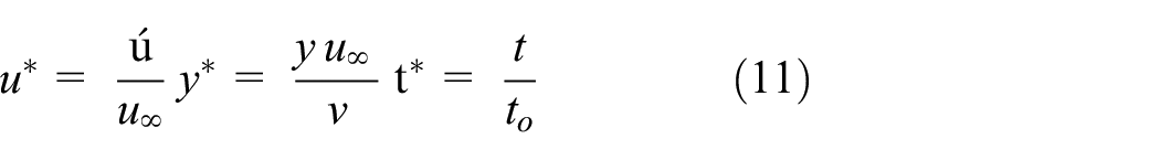
By substituting equation (11) in equation (10), the following equation results:

$$\frac{\partial {\mathrm{u}}^{*}}{\partial {\mathrm{t}}^{*}}=\mathrm{b}(1+\sigma (\mathrm{x}))\frac{{\partial }^2{\mathrm{u}}^{*}}{\partial {{\mathrm{y}}^{*}}^2}$$

(12)

This is a second order partial differential equation and homogeneous. The following similarity transformation is introduced to reduce the partial boundary layer equation (PDE) to an ordinary equation (ODE) with a single independent variable. $\mathrm{\eta }=\frac{A{y}^{*}}{t^{{*}^n}},f\left(\mathrm{\eta }\right)={\mathrm{u}}^{*}$ ;

Substituting in equation (12) the following equation is obtained:

$$f^{``}+\frac{\mathrm{\eta }}{2\mathrm{b}(1+\sigma (\mathrm{x}))\mathrm{A}}{f}^{`}=0$$

(13)

To simplify the equation, A is assumed to be $\frac{1}{\sqrt{2}}$ so the governing equation becomes:

$$f^{``}+\frac{\mathrm{\eta }}{b(1+{\sigma }^2\left(\mathrm{x}\right))}{f}^{`}=0\mathrm{and}\mathrm{\eta }=\frac{y}{\sqrt{2vt}}$$

(14)

Equation (14) is a linear homogeneous second order ordinary differential equation and can be adopted as a replacement to the partial differential equation (6). After several mathematical manipulations done on equation (14) in order to solve it, the following equation is obtained:

$$\mathrm{u}=\mathrm{erf}\left(\frac{\mathrm{\eta }}{\sqrt{2b}(1+{\sigma }^2\left(\mathrm{x}\right))}\right)*\left(u_{\infty }\right)-\frac{p_0\cos \left(\mathrm{nt}\right)}{n}$$

(15)

Equation (15) shows the laminar flow for (b = 1) and turbulent flow for (b > 1) for the wind speed inside boundary layers. It also shows the effect of oscillating pressure gradient for different wind boundary layers. The wind power extracted by the rotor blades can be calculated under the effect of the fluctuating pressure gradient by the following equations.

$$P\left(u(0,R)\right)=\frac{1}{2}\mathrm{\rho }A{u}^3(0,R)\mathrm{Cp}=\frac{1}{2}\mathrm{\rho }\mathrm{cp}{\int }_{A1}^{A2}{u}^3\mathrm{dA}$$

(16)

Here, A is the wind turbine swept area surface (m²), Cp is the power coefficient (dimensionless).

The potential power is calculated by considering the integration on turbine blades from the center to the outside radius where area is (2πrdr) and the radius changes from 0 to R.

$$\begin{array}{c}P\left(u(0,R)\right)=\frac{1}{2}\mathrm{\rho }\mathrm{cp}\hfill \\ {\int }_{r1}^{r2}{(\mathrm{erf}\left(\frac{\mathrm{\eta }}{\sqrt{2b(1+\sigma \left(x\right))}}\right)*\left(u_{\infty }\right)-\frac{p_0\cos \left(\mathrm{nt}\right)}{n})}^{3}2\pi \mathrm{rdr}\hfill \end{array}$$

(17)

Rewriting equation (17) with the dimensionless variable $\mathrm{\eta }$ and replacing (y) by (r + H_b) in equation (15) and integration limits across rotor blades between $\mathrm{\eta }=\frac{(r+H_b)}{\sqrt{2\mathrm{vt}}}$ and hence $d\mathrm{\eta }=\frac{1}{\sqrt{2\mathrm{vt}}}\mathrm{dr}$ and ${\mathrm{\eta }}_1=\frac{H_b}{\sqrt{2\mathrm{vt}}}$ and ${\mathrm{\eta }}_2=\frac{r+H_b}{\sqrt{2\mathrm{vt}}}$ gives the power output as:

Where H_b represents the wind turbine hub height (m).

$$\begin{array}{c}P\left(u(0,R)\right)=\frac{1}{2}\mathrm{\rho }\mathrm{cp}\hfill \\ {\int }_{r_1}^{r_2}{(\mathrm{erf}\left(\frac{\mathrm{\eta }}{\sqrt{2b(1+{\sigma }^{2\left(\mathrm{x}\right)})}}\right)*\left(u_{\infty }\right)-\frac{p_0\cos \left(\mathrm{nt}\right)}{n})}^3\hfill \\ 2\pi \sqrt{2vt}(\mathrm{\eta }\sqrt{2vt}-H_b)d\mathrm{\eta }\hfill \end{array}$$

(18)

This power can be reduced to power calculated without fluctuating pressure effects by setting P_o = 0 and the equation becomes:

$$\begin{array}{c}P\left(u(0,R)\right)=\frac{1}{2}\mathrm{\rho }\mathrm{cp}\hfill \\ {\int }_{{\mathrm{\eta }}_1}^{{\mathrm{\eta }}_2}{(\mathrm{erf}\left(\frac{\mathrm{\eta }}{\sqrt{2b(1+{\sigma }^{2\left(\mathrm{x}\right)})}}\right)*\left(u_{\infty }\right))}^{3}2\pi \sqrt{2vt}(\mathrm{\eta }\sqrt{2vt}-H_b)d\mathrm{\eta }\hfill \end{array}$$

(19)

The ratio between the above two versions is an efficient way to study the effect of pressure gradient fluctuations on the output power of wind turbine and is adopted throughout this study. Actual data from a selected wind turbine data sheet has been used in the study simulations. The wind turbine model used is GE 3.6 – 137 – 50/60 Hz manufactured by GE Energy (USA) which has the following technical specifications (Table 1):

Table 1.

Technical specifications of GE 3.6 – 137 wind turbine.

Rated power	3.6 MW
Hub height	110 m
Rotor diameter	137 m
Rotor swept area	14,741 m2
Tip speed	82 m/s
Number of blades	3
Generating principle	Double-Fed Induction Generation (DFIG)
Power regulation	Asynchronous pitching
Grid standard frequency	50 and 60 Hz
Cut-in wind speed	3 m/s
Cut-off wind speed	25 m/s, in a 600-s time interval

The calculated power curve of the GE 3.6 – 137 – 50/60 Hz wind turbine model at an average air density of 1.225 kg/m³ and medium turbulence intensity is illustrated in Figure 3.

Figure 3.

GE 3.6 – 137 power curve.

Results and discussions

Laminar flow condition simulations

The results of several simulations under laminar flow conditions are presented in this section. To model the laminar flow in MATLAB, the variables in equation (15) have been defined as follows:

• b = 1 represents laminar flow, where b = 1 +  ${\epsilon }_{\mathrm{m}}^{+},$ and ${\epsilon }_{\mathrm{m}}^{+}$ is the dimensionless eddy

• viscosity defined by ${\epsilon }_{\mathrm{m}}^{+}$  = ε_m/ $\mathrm{\nu }$ .

• U_∞ = 5 represents the maximum velocity of air stream (m/s).

• n = 1 represents the number of air pressure gradient fluctuation cycles.

• P_o = 0.1 represents the air pressure gradient fluctuation amplitude.

• $\mathrm{\rho }$  = 1.2 represents air density.

• $v=1.8*{10}^{-5}$ represents air kinematic viscosity.

• $\mathrm{cp}$  = 0.35 represents the efficiency of wind turbine in converting wind’s kinetic energy into electrical energy.

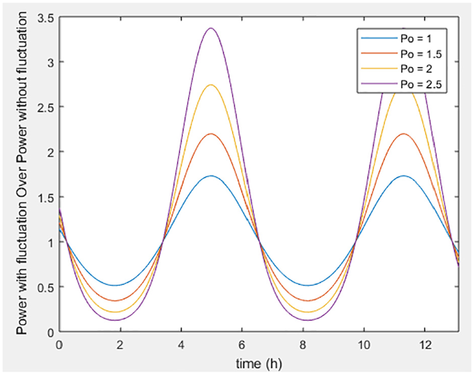
Figure 4 illustrates the power ratio against time (a period of 13 h was chosen) at different (P_o) levels, without taking into consideration the effect of the corrugated surface (CS). It can be noted that as the air pressure gradient amplitude (P_o) is increased, the maximum values of the power ratio is increased as well. It is worth mentioning that the maximum values (peaks) are also increased while the minimum values (troughs) are decreased; this is due to the fact that the air wave form is modeled as a sinusoidal wave in the transformation. This leads to higher output power at some moments and lower output power for other moments, as P_o is increased.

Figure 4.

Power ratio versus time at different (P_o) without CS.

Figure 5 shows the ratio of output power with air pressure gradient fluctuation over output power without air pressure gradient fluctuation against time (a period of 13 h was chosen) at different (P_o) levels, taking into consideration the effect of corrugated surfaces. The corrugated surface has been modeled as a cosine wave. Here, x is taken to be 0.25, representing the wind turbine positioned at Π/4 on the x-axis with respect to the starting point of the cosine wave which is zero. As can be seen, the results for all levels of P_o are the same as those in case of no corrugated surface, as the position of x = 0.25 reduces the corrugated surface equation to 1; hence it has no effect on the final results.

Figure 5.

Power ratio versus time at different (P_o) with CS effect (X = 0.25).

Figure 6 presents the ratio of output power with air pressure gradient fluctuation over output power without air pressure gradient fluctuation against time (a period of 13 h was chosen) at different (P_o) levels, taking into consideration the effect of corrugated surfaces. The corrugated surface has been modeled as a cosine wave. Here, x is taken to be 0.5, representing the wind turbine positioned at Π/2 on the x-axis with respect to the starting point of the cosine wave which is zero. As can be seen, the results for all levels of P_o are the same as those in the case of no corrugated surface impact, as the flow is laminar.

Figure 6.

Power ratio versus time at different (P_o) with CS effect (X = 0.50).

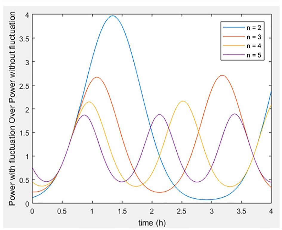
Figure 7 shows the behavior of the power ratio over a period of 13 h in response to several pressure gradient oscillation frequency (n) levels. At small levels of (n) the maximum levels of the power ratio are higher than those at lower (n) levels; however, the minimum levels are higher. This is because the pressure gradient fluctuations are sinusoidal waves. As the (n) value is increased the power peaks are decreased, while the power troughs are still higher than the troughs at lower (n) values. The power is decreased because of adverse pressure gradient frequency oscillations inside the boundary layer. Also increasing the oscillation frequency reduces the contact time between the air stream and the turbine blades.

Figure 7.

Power ratio versus time at different (n) without CS.

Figure 8 illustrates the power ratio response to different levels over 13 h, when taking into consideration the corrugated surface effect. Here, x is taken to be 0.25, representing the wind turbine positioned at Π/4 on the x-axis with respect to the starting point of the cosine wave which is zero. It can be noted that the effect of the corrugated surface is negligible at the position of x = 0.25.

Figure 8.

Power ratio versus time at different (n) with CS effect (X = 0.25).

Figure 9 presents the power ratio with time at different levels of (n). It can be seen that the corrugated surface did not affect in any way the power response to the variation in the pressure gradient oscillation as the flow is in its laminar region.

Figure 9.

Power ratio versus time at different (n) with CS effect (X = 0.50).

Turbulent flow condition simulations

The results of several simulations under turbulent flow conditions are presented in this section. To model the turbulent flow in MATLAB, the variables in equation (15) have been defined as follows:

• b = 15,000 represents turbulent flow.

• Uinfinity = 30 represents the maximum velocity of air stream (m/s).

• n = 3 represents the number of air pressure gradient fluctuation cycles.

• P_o = 4 represents the air pressure gradient fluctuation amplitude.

• v = 1.8 × 10−5 represents air viscosity.

• ρ = 1.2 represents air density.

Figure 10 shows the power ratio (output power with air pressure gradient fluctuation over output power without air pressure gradient fluctuation) against time at different levels of (P_o), without taking into consideration the corrugated surface (CS) effect. The simulation was done for a period of 4 h. The higher the (P_o) the higher the output power peaks, while the troughs are lower as the wave is sinusoidal; this is due to favorable pressure forces moving across turbine blades.

Figure 10.

Power ratio versus time at different (P_o) without CS.

Figure 11 presents the power ratio against time for different values of P_o. It can be seen that the corrugated surface had no effect at the position of X = 0.25 and reduced the corrugated surface equation to ordinary surface.

Figure 11.

Power ratio versus time at different (P_o) with CS effect (X = 0.25).

Figure 12 demonstrates the effect of CS on the output power ratio in the turbulent flow regime. It can be easily noted that the power peaks are increased by almost the double when compared to the no CS effect simulation.

Figure 12.

Power ratio versus time at different (P_o) with CS effect (X = 0.5).

Figure 13 illustrates the power ratio against time at several (n) levels, without taking into consideration the effect of corrugated surfaces. As the value of (n) is increased the power ratio peaks is decreased because the increasing the airwave’s oscillation frequency reduced the time the wind turbines blades remain in contact with the air stream.

Figure 13.

Power ratio versus time at different (n) without CS.

Figure 14 presents the power ratio versus time over a period of 4 h with the corrugated surface effect taken into consideration. However, it can be noted that CS has absolutely no effect on the final power output as the position of X = 0.25.

Figure 14.

Power ratio versus time at different (n) with CS effect (X = 0.25).

Figure 15 clearly demonstrates that the corrugated surface doubled the output power ratio peaks over the chosen period of simulation.

Figure 15.

Power ratio versus time at different (n) with CS effect (X = 0.5).

Figure 16 shows the energy ratio against P_o at several levels of turbulence (b), without the corrugated surface effect. It can be noted that as the P_o is increased so did the energy ratio. Also, as the turbulence level is increased the energy ratio is increased; this is due to favorable inertia forces between fluid layers attacking wind turbine.

Figure 16.

Energy ratio versus P_o at different (b) without CS.

Figure 17 illustrates the energy ratio against P_o at several levels of turbulence (b), considering the corrugated surface. However, it can be noted that CS has absolutely no effect on the final power output as the position of X = 0.25 reduces the corrugated surface equation to 1; hence it has no effect on the final results.

Figure 17.

Energy ratio versus P_o at different (b) with CS effect (X = 0.25).

Figure 18 demonstrates that the corrugated surface impacts strongly affected the energy ratio, as it is increased the output is increased several times when compared to the no CS effect case.

Figure 18.

Energy ratio versus P_o at different (b) with CS effect (X = 0.50).

Conclusions

In this study, the effects of fluctuating pressure gradients and complex terrains on wind turbines power output are studied. Technical specifications from GE 3.6 – 137 wind turbine model have been used, such as the Hub Height and the Rotor Diameter. A theoretical model is built up by using continuity, transient momentum, wind turbine equations, and corrugated surface equations. The impact of fluctuating pressure gradients and corrugated surfaces has been analyzed under laminar and turbulent flow conditions. Two case studies were run in the laminar region; power ratio versus time at different (P_o) levels and power ratio versus time at different (n) levels. Each case study was ran without and with the corrugated surface effect. For the cases including the corrugated surface, two main scenarios have been investigated; when X = 0.25 and X = 0.50. The corrugated surface wave amplitude (α) was chosen to be 0.5 and this value was kept fixed in all scenarios.

After running these equations in several case studies in MATLAB, it can be concluded that:

1. For all cases in the turbulent flow condition presents generally higher output power when compared to those analyzed under the laminar condition. Also, as the air pressure gradient amplitude (P_o) is increased the output power is also increased. This holds true in both laminar and turbulent flow.

2. In addition, as the pressure gradient oscillation frequency (n) is increased the output power ratio is decreased; this is because of the adverse pressure gradient frequency oscillations inside the boundary layer and is applied to laminar as well as turbulent flow.

3. Furthermore, the power ratio is increased greatly as the turbulence level is increased, in the condition of turbulent flow.

4. Regarding the corrugated surface, simulations showed it has almost no impact on the output power in the laminar region as the boundary layer thickness in laminar flow is around three meters and the velocities after this limit are the same. Its impact is only visible in the turbulent region.

5. The corrugated surface impacts the power output according to the turbine position; that is, when the turbine is sited at some positions it may have no effect on the output, while at other positions it may greatly impact the power. In addition, it increased the power ratio by almost one and a half and doubled it for several levels of (P_o) and more than doubles it for different values of (n).

6. Furthermore, the impact of corrugated surfaces on the output is much stronger at higher levels of turbulence when compared to its impact at lower turbulence level.

Recommendations

In this work, the effect of corrugated surfaces and the fluctuating pressure gradient on the output of wind turbines has been determined through studying different MATLAB simulations. A useful suggestion for future studies would be to investigate how the turbine performance changes when varying the geometry of the corrugated surface; that is, to model the corrugated surfaces using a combination of sinusoidal waves representing hilly terrains and square waves representing buildings. Another recommendation would be to find a mathematical equation that relates the corrugated surface parameters (amplitude, wavelength, and wind turbine position) to the expected power output. Also, it is recommended to conduct experiments on real wind turbines installed in operational wind farms or to do tests in experimental wind tunnels and compare the results to those obtained in this work, in order to calculate the error margin between real and simulated output.