Sage Journals: Discover world-class research

Abstract

As a widely used core component of hydropower generation, the stable and safe operation of the Francis turbine plays a very important role in engineering applications. Therefore, the effects of different rotor blade numbers on the hydraulic performance and flow control of the draft tube of the Francis turbine are of great research value. This paper focuses on the rotor blade number 13, 14, 15, 16, and 17 in the prohibited and stabilized operating zones, each of which is taken as a working condition point. (Condition α_ref -H_M and Condition 2α_ref -H_M). Computational Fluid Dynamics (CFD) numerical simulations were performed and analyzed. In terms of hydraulic performance, the increase in the number of blades increases the efficiency and power of the turbine under Condition α_ref -H_M by 2.26% and 0.0021 MW respectively. The efficiency and power of the turbine under Condition α_ref -H_M is also elevated, with the efficiency reaching a maximum of 91.77% at blade number 15, and the power of the same turbine reaching a maximum of 0.182 MW at runner blade number 13. From the 3D flow analysis of the turbine, the increase in the number of blades does not significantly change the flow state of the turbine’s draft tube. By defining the turbulence energy E, the fast Fourier transform of the turbulence energy signals on the two monitoring surfaces of the draft tube is used to obtain its main frequency, and the amplitude and phase at the typical main frequency are visualized, through which we can analyze the vortex band motion state on the two monitoring surfaces of the draft tube, and speculate the change of pressure pulsation of the draft tube. Such an analysis method has a guiding significance for us to improve the performance and stability of the turbine, which can be achieved by increasing or decreasing the number of blades.

Keywords

CFD Francis turbine runner blade number draft tube performance and flow control

Introduction

Hydraulic energy was the first clean energy source¹ to be developed for large-scale utilization by mankind. Under the influence of current environmental and climatic factors, clean energy such as wind, solar, ocean energy and other forms of energy are becoming more and more widely used.^2,3 However, to continue to improve the utilization of water energy technology, the development of more efficient and stable equipment is still the focus of our efforts. Francis turbine is the main equipment for the utilization of water energy and power generation in the middle and high water head.^3,4 Its efficiency is high and the high efficiency zone is very wide, but the stability of operation under full load has always been a problem to be solved. Due to the fluid characteristics of water, it is extremely difficult to mechanically realize its control.⁵ Francis turbine adopts a spiral case and stay vane to collect water flow, and uses guide vane to regulate the flow rate and flow.^6,7 This makes the runner very good for energy conversion, and the draft tube downstream of the runner plays a good role in energy recovery. At present, the highest efficiency of the world’s leading large Francis turbine can reach 93%∼95% level, and it has been used stably for a long time in the Three Gorges Power Station, Baihetan Power Station and other occasions.^8–10

When it comes to the stability of the Francis turbine, it is important to note that the runner blades are not adjustable in angle. In the process of head change, the flow will also change accordingly. runner can adapt to the incoming flow well under the rated condition, but with the shift of the condition, the working condition of the runner is no longer ideal.^11–13 Currently, undesirable flow occurs at the runner inlet, the middle of the blade passage, and the runner outlet, respectively. The undesirable flow at the runner inlet mainly causes pressure pulsation in the vaneless region, which is usually the strongest region of hydraulic excitation. Ye et al.¹⁴ conducted a study of pump-turbine vaneless region unsteady flow with different blade passage inclinations. unit vaneless region unsteady flow characteristics with different blade passage inclinations were numerically simulated. The results show that the large blade tilted runners change the flow near the trailing edge of the blade and in the vaneless region in space and time, which is favorable to improving the flow stability. Lu et al.¹⁵ studied the pressure fluctuation characteristics of a pump-turbine under runaway conditions, based on Q-criterion vortex identification and local entropy generation rate, the vortex moving in the vaneless and runner region interacts with the runner blade, which mainly affects the pressure fluctuation eigenfrequency of the runner. Trivedi et al.¹⁶ studied the pressure fluctuation characteristics of two Francis turbine prototypes with unsteady pressure fluctuations during load change and startup. The results showed that the amplitude of the asynchronous pressure pulsations was 20 times smaller than the amplitude of the synchronous component in the vertical axis turbine, however, the amplitude of the asynchronous pressure pulsations was two times smaller than the amplitude of the synchronous component in the horizontal axis turbine. The amplitude of the synchronous pressure pulsation is almost twice as much as the asynchronous component during the load variation. The middle of the blade passage is mainly presented in the form of vortex in the impeller channel, which mainly triggers the pressure pulsation in the middle of the impeller channel with the force sympathetic to the blades and damages. Through numerical analysis of pressure fluctuations caused by eddy currents between blades in the model of Francis flow turbine, Zuo et al.¹⁷ found that pressure fluctuations of different frequencies were respectively caused by early and developed blade vorticity in the Hill diagram of model flow path parameters. It was found that the pressure fluctuations at different frequencies were caused by early and developing vortices in the blade channel, respectively. Yamamoto et al.¹⁸ used the numerical simulation results to compare three different operating conditions to study the flow structure in the runner blade channel. The results show that the flow inside the runner is characterized by a significant development of recirculation flow on the hub near the runner outlet under partially loaded operation. The runner outlet is connected to the draft tube and the flow is essentially uncontrolled in the circumferential direction, triggering vortex rope and low-frequency pulsations. Jin et al.¹⁹ investigated that when the turbine deviates from the optimum efficiency conditions and is partially loaded, the presence of a spiral vortex band in the center of the draft tube can lead to unstable operation, and they monitored the draft tube pressure pulsation by large vortex simulation. The results show that the draft tube vortex rope can be categorized into spiral vortex, debris vortex and recombination vortex. Zhou et al.²⁰ proposed a new method to mitigate the draft tube vortex rope, which used a conical diffuser to mitigate the vortex rope, it was concluded that the inclined conical diffuser has a significant role in reducing the draft tube vortex rope and disrupting the development of vortex rope. Anup et al.²¹ numerically analyzed the vortex at the outlet of the flow channel to produce a spiraling draft tube vortex band, which induces undesirable flow characteristics. The related analysis was designed to predict the non-constant vortex banding behavior of the draft tube outlet and the flow instability that occurs in a Francis turbine under part-load operation. In general, the flow field pulsations in the vaneless region and the middle of the blade passage are easy to control due to the overlap with the blade position. It is only necessary to improve the blade profile and angle to have good control of the flow. Although the control methods are different under different conditions in different turbines, a reasonable direction can be found after a few attempts. However, the flow and pressure pulsations at the runner outlet and draft tube are not easy to control due to the lack of flow constraints in the circumferential direction. In this case, controlling the flow by improving the number of blades and blade angle becomes feasible. However, its effect on performance and flow pulsations, sometimes the laws are not clear and need to be studied. Wen et al.²² focused on the effect of blade number on the wake flow of a small lifting horizontal-axis wind turbine with a diameter of 0.18 m through large eddy simulation and optimal mode decomposition. The results show that an increase in the number of blades leads to the emergence of interharmonic modes with lower energy than the mean flow pattern. Li et al.²³ aimed to investigate the flow dynamics of a reversible pump turbine (RPT) and the associated runner inlet pressure pulsations under non-operating conditions, as well as the effect of the number of runner blades on the flow dynamics of the RPT. The results show that the flow channel flow instability and machine flow instability decrease with the increase in the number of blades, and the rotor blade number has a significant effect on the rotor inlet pressure pulsations, with 9 and 10 blades corresponding to the lowest and the highest pulsations, respectively. Ketata et al.²⁴ investigated the effect of the number of blades using the latest state-of-the-art 3D-CFD code to improve the performance and further reduce sort of generation. The number of blades was varied from 3 to 15 and the results showed that as the number of blades increased, the efficiency was higher and the losses in the blade runners were less. Yang et al.²⁵ numerically investigated the PAT unsteady pressure field for different numbers of blades. The results show that increasing the number of blades can be effective in lowering the pressure pulsation amplitude. Singh and Nestmann²⁶ proposed a holistic theoretical model to reveal the function of performance parameters inside the flow channel and tried to establish a physical relationship between two design parameters (blade height and number of blades) and the performance parameters. The results show that as the number of blades increases, the change in the direction of the relative flow vector at the outlet of the runner leads to a sharp decrease in the runner efficiency, a decrease in the net momentum and an increase in the axial velocity.

The focus of this paper is to investigate the effect of the number of runner blades on the performance of a Francis turbine, focusing on the performance of the turbine in the range of the high efficiency zone, and focusing on the pressure pulsation characteristics in the case of unstable flow in the tailrace pipe in the deviated operating conditions. In this paper, the performance and pressure pulsation test results are combined with corresponding computational fluid dynamics simulations to carry out flow analysis and trace back the pressure pulsation. This study provides a strong support for improving the operational stability of Francis turbines and hydropower plants.

Francis turbine unit

In this paper, a numerical simulation study is carried out for a Francis turbine with different runner blade numbers, which is mainly composed of volute, stay vanes, guide vanes, runner and draft tube. The diameter of the runner D_M is 300 mm, the rated rotational speed n_M is 1450r/min, the rated head H_M is 38.25 m, the rated power P_M is 0.21 MW, and the 3D model of the fluid domain of the turbine is shown in Figure 1, and the detailed parameter data of the turbine are shown in Table 1. In this paper, we mainly focus on the hydraulic performance and flow control of the draft tube under different blade numbers of the runner. We define the turbine efficiency η, power P, see equations (1) and (2):

η = \frac{M ω}{ρ gQH}

(1)

P = M ω

(2)

where M is Torque, ω is Angular velocity, ρ is Fluid density, g is Gravitational acceleration, Q is flow rate, H is head.

Figure 1.

3D model of Francis turbine unit.

Table 1.

Geometric parameters of objective Francis turbine.

Parameters	Value	Unit
Diameter of runner D_M	300	[mm]
Rated rotation speed n_M	1450	[rpm]
Rated head H_M	38.25	[m]
Rated flow rate Q_M	0.604	[m³/s]
Rated power P_M	0.21	[MW]
Guide vane angle α_ref	12	[°]
Runner rotation frequency f_n	1.667	[Hz]
Number of stay vane Z_svM	24	[-]
Number of guide vane Z_gvM	24	[-]
Number of runner blade	13,14,15,16,17	[-]

Numerical setup

Governing equations

In this study, numerical simulations of three-dimensional incompressible fluids have been carried out using the Reynolds time-averaged method, under which the continuity, momentum and total energy equations are given in equations (3)–(5). These three equations are the core of the numerical simulation method. They describe the mass, momentum, and energy transport in the flow field. The equations are solved by discretizing them to obtain important information about the velocity, pressure, and temperature distributions of the flow field.

\frac{\partial \bar{u_{i}}}{\partial x_{i}} = 0

(3)

ρ \frac{\partial \bar{u_{i}}}{\partial t} + ρ \bar{u_{j}} \frac{\partial \bar{u_{i}}}{\partial x_{j}} = \frac{\partial}{\partial x_{j}} (- \bar{p} δ_{ij} + 2 μ \bar{S_{ij}} - ρ \bar{{u_{i}}^{'} {u_{j}}^{'}})

(4)

\begin{matrix} \frac{\partial}{\partial t} (ρ h_{tot}) - \frac{\partial p}{\partial t} + \frac{\partial}{\partial x_{j}} (ρ u_{j} h_{tot}) = \frac{\partial}{\partial x_{j}} (λ_{t} \frac{\partial T}{\partial x_{j}} - \bar{u_{j} h_{sta}}) \\ + \frac{\partial}{\partial x_{j}} [u_{j} (2 μ \bar{S_{ij}} - ρ \bar{u_{i}^{'} u_{j}^{'}})] \end{matrix}

(5)

where u is velocity, p is the pressure, t is time, ρ is density, T is temperature, x is coordinate component, δ_ij is Kroneker delta, µ is dynamic viscosity, S_ij is mean rate of strain tensor, h_sta is static enthalpy, h_tot is total enthalpy, λ_t is thermal conductivity.

In this study, different turbulence models are considered for different flow situations and engineering problems. And different turbulence has different computational complexity and accuracy, and different wall treatments. Therefore, by combining the above considerations, the SST k-w turbulence model is selected in this study, which has a wide range of use and it includes the mechanism of shear stress transport SST, which helps to simulate the flow behavior at the wall. And it combines the advantages of k-ε and k-w turbulence models. Compared with other turbulence models, this turbulence model is more stable, which effectively wall the numerical simulation dispersion or instability. Based on the above advantages, the SST k-w turbulence model was selected as the turbulence forecasting model in this paper. Its turbulent kinetic energy k equation and turbulent dissipation rate w equation are expressed as equations (6) and (7):

\frac{\partial (ρ k)}{\partial t} + \frac{\partial (ρ u_{i} k)}{\partial x_{i}} = P_{k} - \frac{ρ k^{3 / 2}}{l_{k - ω}} + \frac{\partial}{\partial x_{i}} [(μ + σ_{k} μ_{t}) \frac{\partial k}{\partial x_{i}}]

(6)

\begin{matrix} \frac{\partial (ρ ω)}{\partial t} + \frac{\partial (ρ u_{i} ω)}{\partial x_{i}} = C_{ω} P_{ω} - β ρ ω^{2} + \frac{\partial}{\partial x_{i}} [(μ_{l} + σ_{ω} μ_{t}) \frac{\partial ω}{\partial x_{i}}] \\ + 2 (1 - F_{1}) \frac{ρ σ_{ω 2}}{ω} \frac{\partial k}{\partial x_{i}} \frac{\partial ω}{\partial x_{i}} \end{matrix}

(7)

l_{k - ω} = k^{1 / 2} β_{k} ω

(8)

Different blade numbers and research objective

We carried out numerical simulation analysis under two operating conditions, Condition α_ref -H_M and Condition 2α_ref -H_M, for the five runner scheme with runner blades of 13, 14, 15, 16, 17, and the specific number of runner blades is shown in Figure 2. In response to the increase in the number of blades, we reduced the thickness of the blades in equal proportions, and we ensured that the total thickness remained unchanged, blades shape did not change. Condition α_ref -H_M exists in the prohibited operation zone of the turbine and Condition 2α_ref -H_M exists in the stable operation zone of the turbine. See Figure 3. Therefore, these two typical conditions are selected.

Figure 2.

Schematic diagrams of different runner blade numbers.

Figure 3.

Schematic diagram of the operating conditions of the unit.

For this paper we define the turbulence energy E, which can be expressed by equation (9), where the turbulent kinetic energy and turbulent vortex frequency are expressed by equations (10) and (11) respectively:

E = \frac{Δ kw}{ρ gQH}

(9)

where Δkw is the peak-to-peak value of the product of turbulent kinetic energy and turbulence eddy frequency.

k = \frac{1}{2} ρ u \cdot u'

(10)

where k is turbulent kinetic energy, ρ is density of the fluid, u is average vector velocity of the fluid. $u'$ is Vortex portion of flow velocity.

ω = \frac{k}{\sqrt{ε}}

(11)

where w is Turbulence Eddy Frequency, k is Turbulence Kinetic Energy, $ε$ is Turbulence Dissipation Rate.

CFD setup with monitoring points

The value simulation calculations rely on ANSYS CFX commercial software and the relevant theories of CFD. The simulation problem is clearly defined, which includes determining the geometry of the problem, the type of flow, the boundary conditions, the fluid medium, and so on. Therefore, we have studied and calculated the turbulent energy of the draft tube of a Francis turbine under typical operating conditions for different number of runner blades based on the consideration of the above problems. In this study, the numerical simulation of the fluid medium is water at 25°C and is carried out at a reference air pressure of 1 Atm. The inlet of the volute is identified as the inlet of the whole fluid domain and set as the total pressure inlet boundary condition, and the outlet of the draft tube is identified as the outlet of the fluid domain and set as the mean static pressure outlet boundary condition. The outlet is connected to the atmosphere with a pressure value of 0 Pa. The runner is the only rotating component with a rotational speed of 1450 r/min, and the dynamic reference system is set up between the runner and the guide vanes as well as between the runner and the draft tube, and the static reference system is set up between the rest of the components. A generalized grid interface GGI model is used for data transfer between different interfaces. The turbulence model is selected as SST k-w, and the explanation of the key rationale is carried out in the previous section.

For the computational solution setup, both steady and unsteady simulations were performed in this study. The minimum number of iteration steps for the steady computation is 1000, and the result is used as the initial file for the unsteady computation. The unsteady computation is iterated for 180 steps for each runner cycle, and each step is iterated 10 times for a total of 10 cycles. The convergence criterion of the numerical simulation is the continuity equation, and the root-mean-square residuals of the momentum and energy equations are less than 1 × 10⁻⁵. Many monitoring points are arranged in the draft tube close to the inlet section, and 1000 monitoring points are arranged in each monitoring surface to form the detection surface 1 and 2, which are shown in Figure 4. Turbulence kinetic energy k, as well as turbulence vortex frequency w, are mainly monitored.

Figure 4.

Schematic layout of monitoring surfaces.

Determination and check of Mesh

In CFD numerical simulation, meshing is a very important step and they have a crucial role in the accuracy and reliability of the simulation. Therefore, a combination of structured and unstructured meshes is used in our study. Based on ICEM CFD and TurboGrid commercial software, the fluid domain of the Francis turbine is discretized, and the mesh element type and number of mesh element for each component are shown in Table 2. And the mesh irrelevance is checked based on Richardson’s extrapolation.²⁷

Table 2.

Type of grid and number of grids for each component of the turbine.

Component	Mesh element type	Mesh element number
Volute	Tetrahedral cell grid	247,915
Stay vane	Tetrahedral cell grid	1,400,646
Guide vane	Tetrahedral cell grid	1,604,155
Runner	Hexahedral cell grid	343,060
Draft tube	Tetrahedral cell grid	1,348,422
Total		4,944,198

For this purpose, three grid schemes with different number of mesh elements are prepared in this paper, namely coarse (N1 = 7,042,620), medium (N2 = 275.3686), fine (N3 = 1,110,522), there is a significant difference in resolution between the three grid schemes. CFD simulations were performed using grid schemes with different resolutions, ensuring that the mesh scheme was used as the only variable and the rest of the parameters were kept constant. For the obtained numerical simulation results, the GCI method is used to calculate the grid convergence index, and the extrapolated values of GCI are plotted in Figure 5. The refinement factor of medium and coarse is 1.3535, and the value of GCI is 0.0003%. the refinement factor of fine and medium is 1.3675, and the value of GCI is 0.039%, which all satisfy the convergence requirements. From Figure 5, we can see that the three sets of grid programs with different resolutions have better convergence, so in this paper, considering the computational resources and computational accuracy, we learned the Fine grid program as the final computational program, the total number of grid cells is 4,944,198. See Figure 6.

Figure 5.

Details of grid independence check.

Figure 6.

Mesh delineation and local enlargement of a Francis turbine unit.

Validation of numerical results

Figure 7 shows the comparison between the experimental pressure pulsations and the numerical simulation results for the Condition 1.12 α_ref-0.735 HM. We chose the 13-blade scheme for the test and comparison of the numerical simulation. The main selection was the comparison of the pressure pulsation peak value in the leafless area, the draft pipe and the volute. We found that the error between the test and the numerical simulation results was less than 10%, and we believed that such error was within our acceptable range. Therefore, we use numerical simulation instead of test to analyze the relevant hydraulic performance and flow control.

Figure 7.

Comparison of pressure pulsation amplitude between test and numerical simulation (Condition 1.12 α_ref-0.735 HM).

Results of performance analysis

Efficiency and power comparisons

We selected two typical working conditions, Condition α_ref -H_M and Condition 2α_ref -H_M, for numerical simulation analysis, and compared and analyzed the changes of the efficiency and power of the turbine under different rotor blade numbers, respectively, see Figures 8 and 9.

Figure 8.

diagram of turbine efficiency and power variation at different number of blades under Condition α_ref -H_M.

Figure 9.

diagram of turbine efficiency and power variation at different number of blades under Condition 2α_ref -H_M.

Figure 8 demonstrates the variation of turbine performance under operating condition α_ref -H_M, firstly, we find that the operating efficiency of the turbine has a significant increase with the increase in the number of blades, from 73.67% for B13 to 75.93% for B17, which is an increase of 2.26%. Although the efficiency of the turbine also increases, the range of increase is not obvious, from 0.0658 MW in the B13 scheme to 0.0679 MW in the B17 blade scheme, with a power increase of 0.0021 MW. From the above data, it is found that the increase in the number of blades of the turbine improves both the efficiency and the power of the turbine under the α_ref -H_M operating conditions.

Figure 9 shows the variation of turbine performance for operating condition α_ref -H_M, we find that the turbine efficiency reaches a maximum of 91.77% at blade number 15 and the turbine operates at a minimum of 91.59% at blade number 16. Similarly, the turbine power reaches a maximum of 0.182 MW at runner blade number 13, and the turbine operates with the lowest power of 0.179 MW at both runner blade numbers 16 and 17. Such evaluation results provide us with guidance on the number of blades in the subsequent optimized design of the turbine.

The internal flow pattern

In this subsection, 3D streamline are used to analyze the turbine flow, which can visualize the complex flow, and by drawing the streamline, it is clear to see how the fluid flows in the 3D space, including the phenomena of swirls, eddies, and separations.

The flow at Condition α_ref -H_M can be seen in Figure 10 for turbines with different number of blades. The distribution of the streamline represents the state of turbulence and the color indicates the flow velocity. Since the flow velocity is more stable at the inlet of the worm shell and the maximum value of the flow velocity exists at the runner with an average value of 26 m/s under the condition of prohibited operation zone, the flow condition in the draft tube becomes worse, and the flow condition in the draft tube is basically similar under the schemes with different numbers of blades, and there is a large number of vortexes as well as chaotic flow conditions, which is related to the formation of the vortex band of the draft tube to a certain extent, and the flow conditions of the two outlets in the are not similar, and the flow condition near the turbulent flow is not similar to that near the worm shell. This is related to the formation of vortex zone in the draft tube, and the two outlets of the draft tube are not similar, and the outlet pipe close to the inlet side of the snail shell obviously flows more strongly. Such a flow condition will cause strong pressure pulsation and noise in the draft tube. Such a flow pattern is not ideal for the operation of the turbine.

Figure 10.

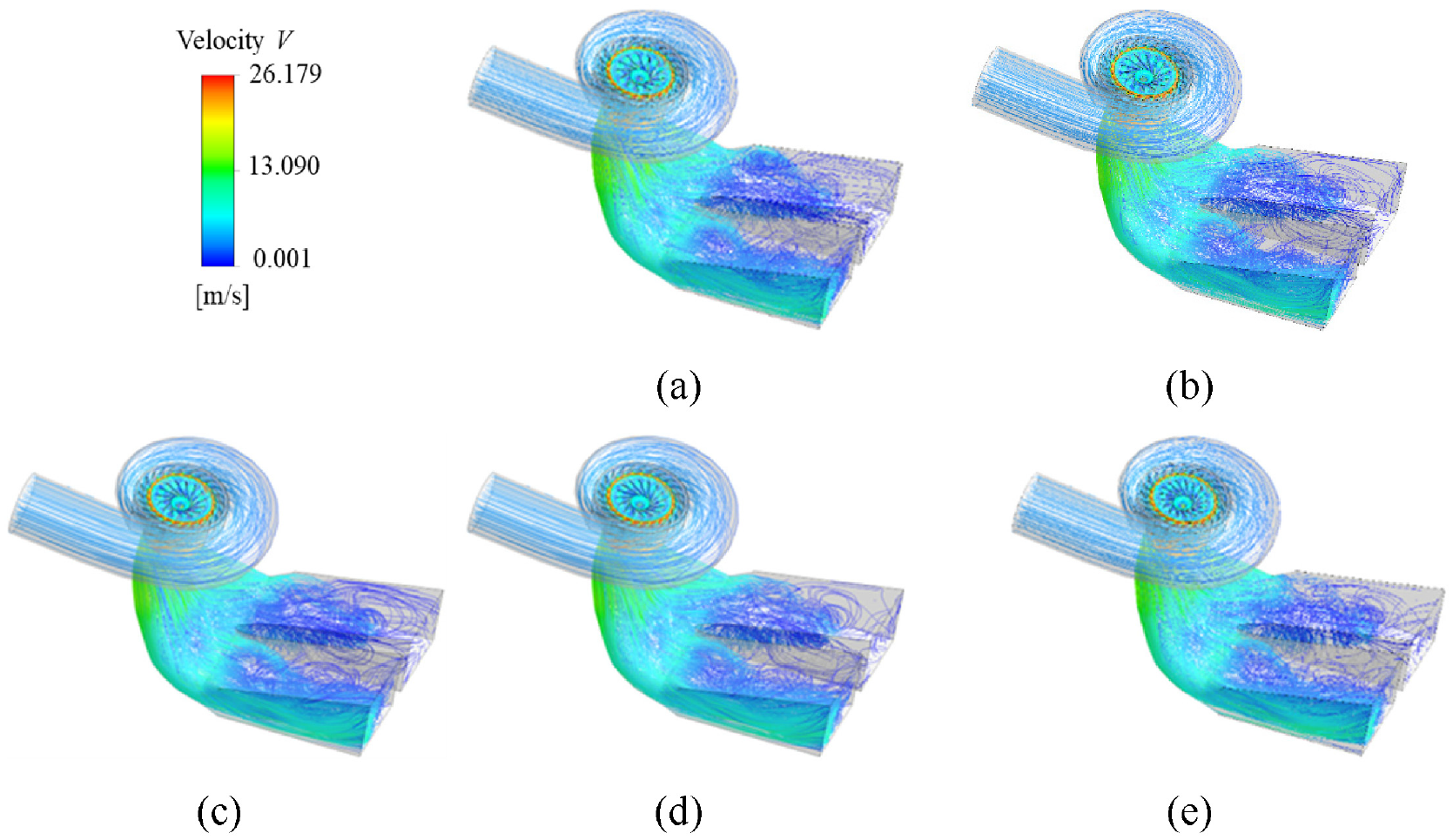
3D flow line diagram of the turbine under Condition α_ref -H_M with different number of blades: (a) B13, (b) B14, (c) B15, (d) B16, and (e) B17.

Figure 11 shows the flow in the turbine with different blade numbers under Condition α_ref -H_M. Since the flow pattern in the turbine with different blade numbers is very stable in terms of flow velocity in the stable operation zone, there is almost no vortex and flow separation. The maximum speed of the rotor reaches about 32 m/s, and the flow pattern in the draft tube is significantly more stable than that in the forbidden operation zone, which is a more ideal flow condition for the stable operation of the turbine, and the pressure pulsation and noise in the draft tube are not too strong.

Figure 11.

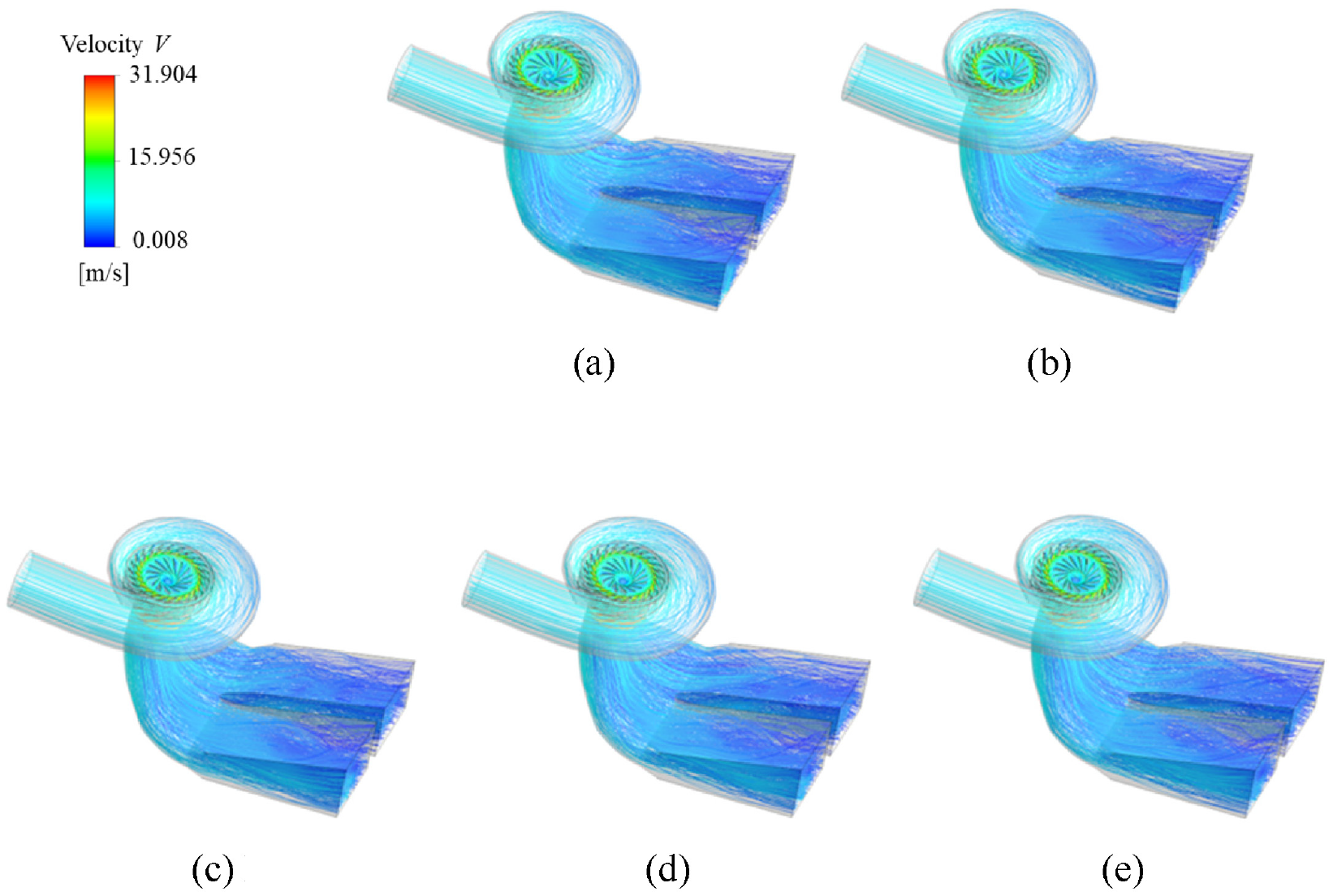
3D flow line diagram of the turbine under Condition 2α_ref-H_M with different number of blades: (a) B13, (b) B14, (c) B15, (d) B16, and (e) B17.

Results of turbulent energy analysis in the draft tube

Main frequency

We have analyzed the dominant frequency of the turbulent energy E signal for typical operating conditions at different blade numbers. Figures 12 and 13 show the dominant frequencies of turbulent energy for two operating conditions at 13 and 14 blade numbers. The dominant frequencies are 0.2 f_n and f_n for the two detection surfaces of Condition α_ref -H_M, and 0.2 f_n, 0.4 f_n, and 0.6 f_n for the two monitoring surfaces of Condition 2 α_ref -H_M, and there is no obvious pattern in the distribution of the dominant frequencies on the two monitoring surfaces.

Figure 12.

Main frequency of two monitoring surfaces for typical conditions under B13.

Figure 13.

Main frequency of two monitoring surfaces for typical conditions under B14.

Figures 14 and 15 show that when the number of blades is increased to 15 and 16, the dominant frequency of turbulence energy E on the two monitoring surfaces under Condition α_ref -H_M appears to be 0.8 f_n, but the overall percentage is small, and the original 0.2 f_n and f_n are still present without any significant change. The dominant frequencies on the two surfaces under Condition 2α_ref -H_M are still 0.2 f_n, 0.4 f_n, and 0.6 f_n. Comparisons with the other vane number scenarios show no significant changes. However, the overall share of the dominant frequency of 0.4f_n tends to decrease.

Figure 14.

Main frequency of two monitoring surfaces for typical conditions under B15.

Figure 15.

Main frequency of two monitoring surfaces for typical conditions under B16.

Figure 16 shows that for blade number 17, the dominant frequency of turbulent energy E at both monitoring surfaces of the draft tube under Condition α_ref -H_M changes significantly, with the dominant frequency of 0.8f_n increasing and the dominant frequency of 0.4f_n decreasing, which is a significant difference from the previous blade scenario. In Condition 2α_ref-H_M the dominant frequencies are still composed of 0.2f_n, 0.4f_n, and 0.6f_n, and no new dominant frequencies appear. Thus, we find that the increase in the number of blades does not significantly affect the dominant frequency of turbulent kinetic energy in the wake pipe in Condition 2α_ref -H_M in the stabilized region, but it influences the forbidden region.

Figure 16.

Main frequency of two monitoring surfaces for typical conditions under B17.

Amplitude of typical frequencies

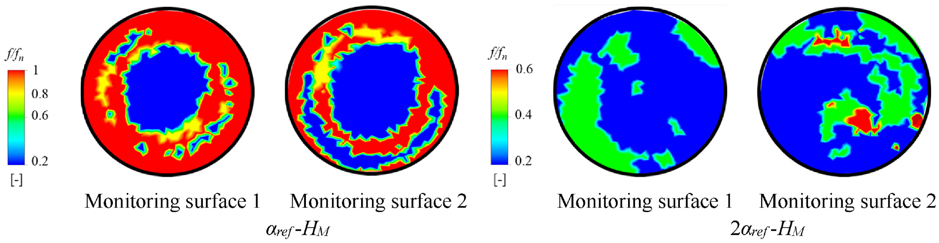
Figure 17 shows the turbulent energy intensity of Condition α_ref -H_M B13 at main frequencies of 0.2f_n and 1f_n. At f = 0.2f_n, the maximum turbulence intensity of monitoring surfaces 1 and 2 is 2.91 × 10⁻⁵, and the high turbulence energy intensity is distributed in the shape of a circle in both monitoring sections of the draft tube, mainly present in the sidewalls of the draft tube, and the turbulence intensity in the center area is the turbulence intensity in the center region is relatively low. At f = f_n, the turbulence intensity in a circle around the monitoring surface 1 is about 5.34 × 10⁻⁵, and the center turbulence energy intensity is almost 0. While the turbulence energy intensity on the monitoring surface 2 is not high at all, and there is a slight region of high turbulence energy on the wall.

Figure 17.

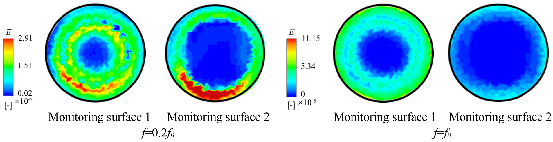
Amplitude of the typical main frequency of the two monitoring surfaces under condition α_ref -H_M B13.

Figure 18 illustrates the distribution of turbulent energy intensity for Condition 2α_ref -H_M B13 at main frequencies of 0.2f_n, 0.4f_n. At f = 0.2f_n, the maximum turbulent energy intensity on the monitoring surfaces 1, 2 is relatively small over the whole monitoring surface, with a maximum value of 6.44 × 10⁻⁵. Most of the turbulent energy intensity is 3.51 × 10⁻⁵ and close to 0. The turbulent energy intensity on the monitoring surfaces 1, 2 decreases significantly at f = 0.4f_n. The rest of the area gives a maximum turbulent energy intensity of 2.73 × 10⁻⁵ as well as most of them are close to zero.

Figure 18.

Amplitude of the typical main frequency of the two monitoring surfaces under condition 2α_ref -H_M B13.

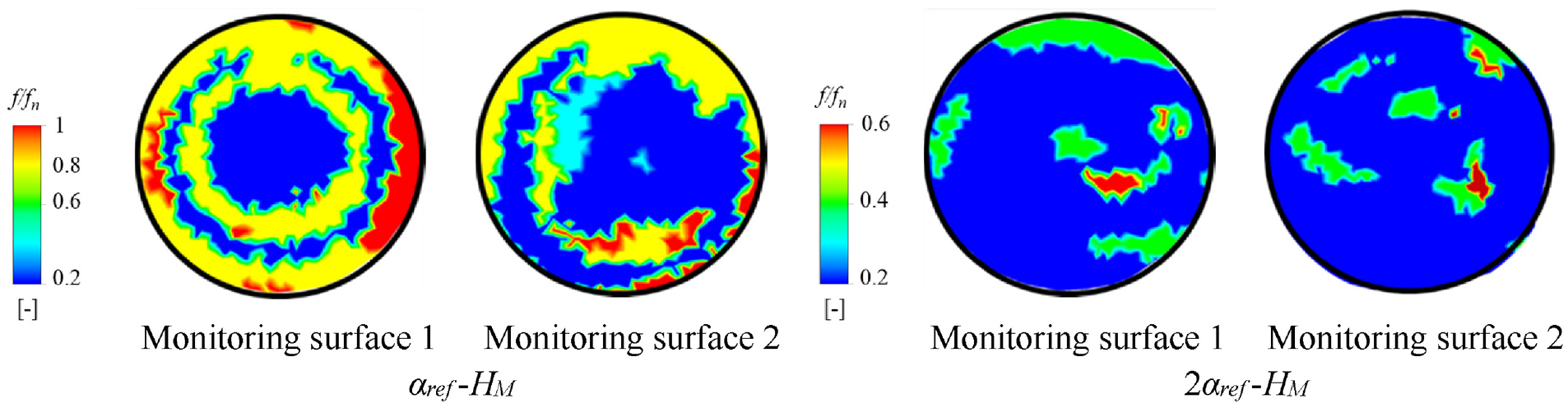
Figure 19 shows the turbulent energy intensity of Condition α_ref -H_M B14 at the main frequency of 0.2f_n, 1f_n. At f = 0.2f_n, the maximum value of turbulence intensity at monitoring surfaces 1, 2 is 2.42 × 10⁻⁵, and the high turbulence energy intensity shows a multi-circular circular shape distributed on the monitoring surface 1 of the draft tube, and the high turbulence energy intensity on the monitoring surface 2 is higher than that on the monitoring surface 1, and mainly exists with the sidewalls of the draft tube, and the center region is relatively low. The high turbulence energy intensity on monitoring surface 2 is higher than that on monitoring surface 1, which mainly exists on the sidewalls of the draft tube, and the turbulence intensity in the center region is relatively low. At f = f_n, the turbulence intensity in the surrounding ring on monitoring surface 1 is about 5.34 × 10⁻⁵, and the center turbulence energy intensity is almost 0. The turbulence energy intensities on monitoring surface 2 are not high, and there is a little bit of high turbulence energy in the draft tube poop wall.

Figure 19.

Amplitude of the typical main frequency of the two monitoring surfaces under condition α_ref -H_M B14.

Figure 20 illustrates the distribution of turbulent energy intensity for Condition 2α_ref -H_M B14 at main frequencies of 0.2f_n, 0.4f_n. At f = 0.2f_n, the maximum turbulent energy intensity on monitoring surfaces 1 and 2 is relatively small over the whole monitoring surface, with a maximum value of 7.12 × 10⁻⁵, and most of the turbulent energy intensity is 3.51 × 10⁻⁵ and close to 0.02. At f = 0.4f_n, the turbulent energy intensity on monitoring surface 1 is 50% smaller than that on monitoring surface 1 with a dominant frequency of 0.2f_n, and the turbulent energy intensity on monitoring surface 2 is also reduced, with only 3.4 × 10⁻⁵, and the turbulent energy intensity of monitoring surface 2 is also reduced. The turbulent energy intensity in the rest of the area is reduced to a maximum of 1.5 × 10⁻⁵ and mostly close to 0. The turbulent energy intensity is reduced by 50% at f = 0.4f_n compared to the 0.2f_n dominant frequency on monitoring surface 1, and the turbulent energy intensity on monitoring surface 2 is reduced to 3.4 × 10⁻⁵.

Figure 20.

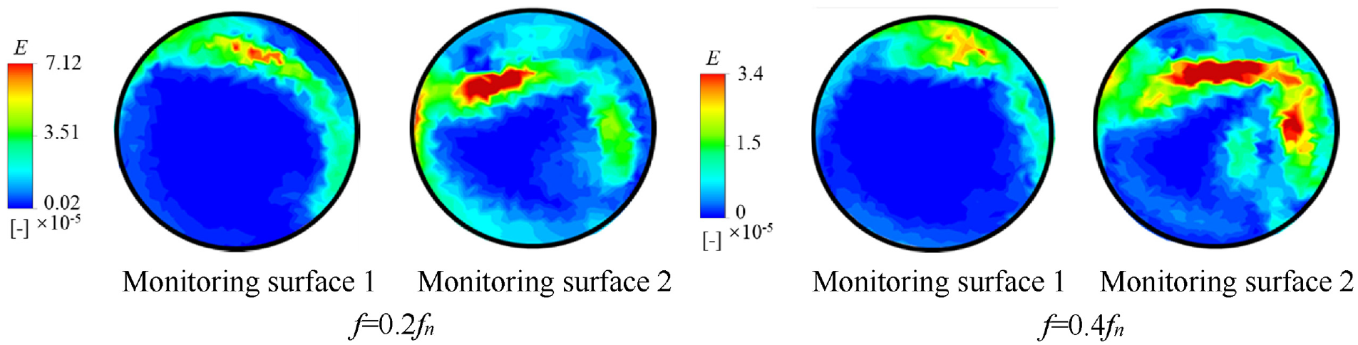
Amplitude of the typical main frequency of the two monitoring surfaces under condition 2α_ref -H_M B14.

Figure 21 shows the turbulent energy intensity of Condition α_ref -H_M B15 at main frequencies of 0.2f_n and 1f_n. At f = 0.2f_n, the maximum turbulent energy intensity of monitoring surfaces 1 and 2 is 2.42 × 10⁻⁵, and the high turbulent energy intensity shows a multi-circular circular shape distributed on the monitoring surface 1 of the draft tube, and the high turbulent energy intensity of monitoring surface 2 is significantly higher than that of monitoring surface 1, about three times higher in size, and mainly exists with the draft tube sidewalls, and the center region is relatively low. The high turbulent energy intensity on the monitoring surface 2 is significantly higher than that on the monitoring surface 1, which is about 3 times higher in size, and mainly exists on the sidewalls of the draft tube, while the turbulent energy in the center region is relatively low. This is related to the motion of the vortex zone in the draft tube. At f = f_n, the turbulence intensity in a circle around the monitoring surface 1 is about 3.34 × 10⁻⁵, and the center turbulence energy intensity is almost 0. The turbulence energy intensity in the monitoring surface 2 is not high, and there is a little bit of high turbulence energy in the draft tube wall, which is basically the same as that in the case of vane numbers 13 and 14.

Figure 21.

Amplitude of the typical main frequency of the two monitoring surfaces under condition α_ref -Figure 22 Amplitude of the typical main frequency of the two monitoring surfaces under condition 2α_ref -H_M B15.

Figure 22 illustrates the distribution of turbulent energy intensity for Condition 2α_ref -H_M B15 at main frequencies of 0.2f_n, 0.4f_n. At f = 0.2f_n, the maximum turbulent energy intensity on monitoring surfaces 1 and 2 is relatively small over the whole monitoring surface, with a maximum value of 5.54 × 10⁻⁵. Most of the turbulent energy intensity is 3.01 × 10⁻⁵ and close to 0.02 × 10⁻⁵. At f = 0.4f_n, the turbulent energy intensity on monitoring surface 1 is reduced by 50% and on monitoring surface 2 is reduced by 200%, compared to that on monitoring surface 1 for the dominant frequency of 0.2f_n. The turbulent energy intensity on monitoring surface 2 is reduced by 200% to 3.26 × 10⁻⁵. The rest of the region gives a turbulent energy intensity of up to 1.54 × 10⁻⁵ and most of it is close to 0. The turbulent energy intensity on monitoring surface 2 is reduced by 200% to 3.26 × 10⁻⁵ at f = 0.4f_n.

Figure 22.

Amplitude of the typical main frequency of the two monitoring surfaces under condition 2α_ref -H_M B15.

Figure 23 shows the turbulent energy intensity of Condition α_ref -H_M B16 at main frequencies of 0.2f_n and 1f_n. At f = 0.2f_n, the maximum value of turbulence intensity at monitoring surfaces 1 and 2 is 2.87 × 10⁻⁵, and the high turbulence energy intensity shows a multi-circular circular shape distributed on the monitoring surface 1 of the draft tube, and the high turbulence energy intensity on monitoring surface 2 is significantly higher than that on monitoring surface 1, which is about 5 times the size of the enhancement, mainly exists with the side wall of the draft tube, and the turbulence intensity in the center region is relatively low. This pattern does not change. At f = f_n, the turbulent energy in a circle around monitoring surface 1 is about 4.34 × 10⁻⁵, and the turbulent energy intensity in the center is almost 0. The turbulent energy intensities on monitoring surface 2 are not high, and there is a little bit of high turbulent energy on the draft tube sidewalls, which is basically the same as that in the case of vane numbers 13, 14, and 15.

Figure 23.

Amplitude of the typical main frequency of the two monitoring surfaces under condition α_ref -H_M B16.

Figure 24 illustrates the distribution of turbulent energy intensity for Condition 2α_ref -H_M B16 at main frequencies of 0.2f_n, 0.4f_n. At f = 0.2f_n, the maximum turbulent energy intensity on monitoring surfaces 1 and 2 is relatively small over the whole monitoring surface, with a maximum value of 4.1 × 10⁻⁵. Most of the turbulent energy intensity is 2.01 × 10⁻⁵ and close to 0.02 × 10⁻⁵. At f = 0.4f_n, compared to turbulent energy on monitoring surface 1, turbulent energy intensity on monitoring surface 2 is significantly enhanced, with about 200% increase to 1.73 × 10⁻⁵. 200% to 1.73 × 10⁻⁵. The rest of the region gives turbulent energy intensities up to 1.04 × 10⁻⁵ and mostly close to zero.

Figure 24.

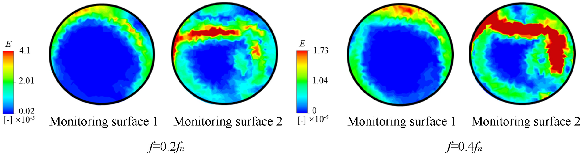
Amplitude of the typical main frequency of the two monitoring surfaces under condition 2α_ref -H_M B16.

Figure 25 shows the turbulent energy intensity of Condition α_ref -H_M B17 at main frequencies of 0.2f_n, 0.8f_n. At f = 0.2f_n, the maximum value of turbulence intensity at monitoring surfaces 1, 2 is 3.27 × 10⁻⁵, and the high turbulence energy intensity exhibits a circular shape distributed as the monitoring surface 1 of the draft tube, and the high turbulence energy intensity on monitoring surface 2 is significantly higher than that on monitoring surface 1, about one times the size of enhancement. The high turbulence energy intensity on the monitoring surface 2 is significantly higher than that on the monitoring surface 1, which is enhanced by about one times in size, and mainly exists on the sidewalls of the draft tube, while the turbulence intensity in the center region is relatively low. At f = 0.8 f_n, the turbulent energy in a circle around monitoring surface 1 is about 2.91 × 10⁻⁵, and the intensity of turbulent energy in the center is almost 0. The intensity of turbulent energy on monitoring surface 2 is not high, and there is a little bit of high turbulence energy on the draft tube wall, and the turbulence energy in the center is almost 0.

Figure 25.

Amplitude of the typical main frequency of the two monitoring surfaces under condition α_ref -H_M B17.

Figure 26 illustrates the distribution of turbulent energy intensity for Condition 2α_ref -H_M B17 at main frequencies of 0.2f_n, 0.4f_n. At f = 0.2f_n, the maximum turbulent energy intensity on the monitoring surfaces 1 and 2 is relatively small over the whole monitoring surface, with a maximum value of 5.14 × 10⁻⁵. Most of the turbulent energy intensity is 3.01 × 10⁻⁵ and close to 0.02 × 10⁻⁵. At f = 0.4f_n, the region of high turbulence energy still exists at the sidewall location and has a maximum value of 4.04 × 10⁻⁵, and most of the monitoring surface has zero turbulent energy value. values of turbulent energy are zero in most areas of the surface.

Figure 26.

Amplitude of the typical main frequency of the two monitoring surfaces under condition 2α_ref -H_M B17.

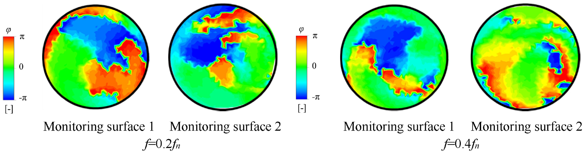
Phase and phase difference

Phase changes in signals are physically important. In the frequency domain, the Fourier variation of a signal represents the amplitude and phase information of the different frequency components of the signal, and the phase tells us how cheap or delayed the signal is at different frequencies. Specifically, the phase of a frequency component indicates the starting point of the signal on the time axis. When the phase of a signal changes, it indicates that the waveform of that frequency component is shifted or offset relative to the time axis.

Figure 27 shows the phase change of the turbulent energy signal of Condition α_ref -H_M B13 at a main frequency of 0.2f_n, f_n. There is no obvious change in the propagation trend of the turbulent energy on the monitoring surface 1 at f = 0.2f_n, and on the monitoring surface 2 we can see a tendency for the signal cycle to span in the middle of the draft tube, and from this we can hypothesize that the change in the turbulent energy from this we can assume that the change in turbulent energy is related to the change in the vortex here. At f = f_n, we can clearly find a clockwise trend of the turbulent energy signal on both monitoring surfaces, and from monitoring surface 1 to monitoring surface 2, we can see that the turbulent energy signal has a visualization of the state of motion at that moment.

Figure 27.

Phase of the typical main frequency of the two monitoring surfaces under condition α_ref -H_M B13.

Figure 28 illustrates the phase variation of the turbulent energy signal for Condition 2α_ref -H_M B13 at the main frequency of 0.2f_n, 0.4f_n. At f = 0.2f_n, the turbulent energy on the monitoring surface 1 tends to move chaotically, which is strongly related to the state of the fluid in this condition, and the chaos on the monitoring surface 2 is reduced, but it is still irregular. At f = 0.4 f_n, the turbulent energy on surface 1 is also chaotic to a certain extent, but the phase change on surface 1 is less drastic than that on surface 2 at 0.2 f_n, and the turbulent energy on surface 2 is more stable, with a slight cycle spanning near the edge wall of the draft tube.

Figure 28.

Phase of the typical main frequency of the two monitoring surfaces under condition 2α_ref -H_M B13.

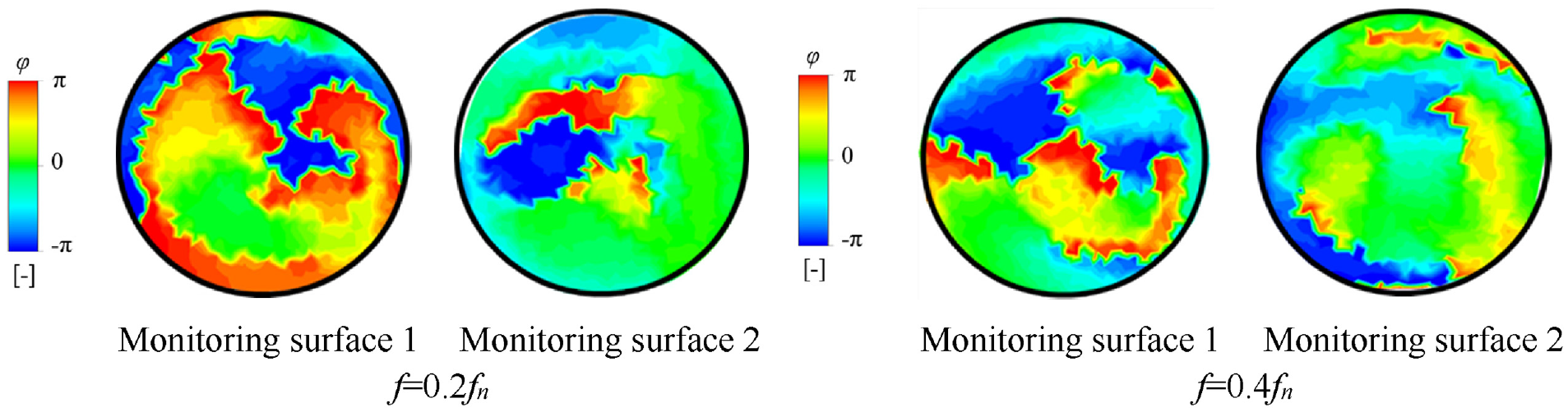
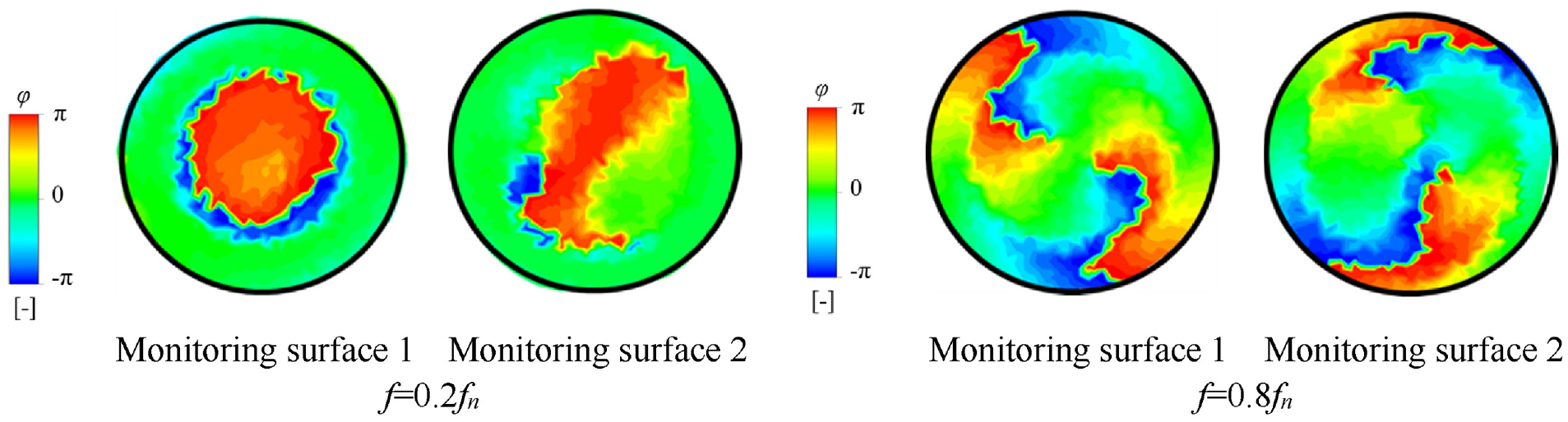
Figure 29 illustrates the phase variation of the turbulent energy signal for Condition α_ref -H_M B14 at a main frequency of 0.2 f_n, f_n. At f = 0.2 f_n, the turbulent energy does not have a clear cycle-spanning flow pattern at monitoring surface 1 as seen through both monitoring surfaces, but a trend toward a cycle-spanning turbulent energy signal with vortex banding motions is clearly seen on monitoring surface 2. At f = f_n, we can see that there is a clear cycle spanning of the phase of the turbulent energy signal with eddy motion, and there is a clear trend on both monitoring surfaces.

Figure 29.

Phase of the typical main frequency of the two monitoring surfaces under condition α_ref -H_M B14.

Figure 30 illustrates the phase variation of the turbulent energy signal for Condition 2α_ref-H_M B14 at main frequencies of 0.2f_n, 0.4f_n. At f = 0.2f_n, the periodic phase changes of the turbulent energy signals on both surfaces 1 and 2 are relatively chaotic. At f = 0.4f_n, the phase changes of turbulent energy signals on both monitoring surfaces are relatively chaotic. We believe that the poor flow condition of the draft tube at both main frequencies in this case is closely related to the vortex zone.

Figure 30.

Phase of the typical main frequency of the two monitoring surfaces under condition 2α_ref -H_M B14.

Figure 31 illustrates the phase variation of the turbulent energy signal for Condition α_ref -H_M B15 at a main frequency of 0.2f_n, f_n. At f = 0.2f_n, the turbulent energy does not have a clear cycle-spanning flow pattern at monitoring surface 1 as seen through both monitoring surfaces, but a trend toward a cycle-spanning turbulent energy with vortex banding motions is clearly seen on monitoring surface 2. At f = f_n, we can see that there is a clear phase period spanning of the turbulent energy signal with eddy motion, with a clear trend on both monitoring surfaces.

Figure 31.

Phase of the typical main frequency of the two monitoring surfaces under condition α_ref -H_M B15.

Figure 32 illustrates the phase variation of the turbulent energy signal for Condition 2α_ref -H_M B15 at main frequencies of 0.2f_n, 0.4f_n. At f = 0.2f_n, the periodic phase variations of the turbulent energy signals at both monitoring surfaces 1 and 2 are relatively slight, with a slight period spanning. At f = 0.4f_n, the phase variation of the turbulent energy signal at monitoring surface 1 is relatively stable, however, the phase variation at monitoring surface 2 is very chaotic.

Figure 32.

Phase of the typical main frequency of the two monitoring surfaces under condition 2α_ref -H_M B15.

Figure 33 shows the phase variation of the turbulent energy signal for Condition α_ref - H_M B16 at a main frequency of 0.2f_n, f_n. At f = 0.2f_n, the turbulent energy is seen to have no significant cycle-spanning flow pattern at monitoring surfaces 1 and 2, with a few phase cycles spanning in the center region, as seen through both monitoring surfaces. At f = f_n, we can see that there is a regular trend in the phase period crossing of the turbulent energy signal with significant swirling motion in both monitoring surfaces.

Figure 33.

Phase of the typical main frequency of the two monitoring surfaces under condition α_ref -H_M B16.

Figure 34 illustrates the phase variation of the turbulent energy signal for Condition 2α_ref -H_M B16 at main frequencies of 0.2f_n, 0.4f_n. At f = 0.2f_n, the periodic phase variations of the turbulent energy signals are present at both monitoring surfaces 1 and 2, which are relatively slight, with a slight period spanning, and occur mainly at the location of the draft tube sidewalls. At f = 0.4f_n, the phase variations of the turbulent energy signals at both surfaces 1 and 2 are chaotic, and there is no clear pattern of phase spanning.

Figure 34.

Phase of the typical main frequency of the two monitoring surfaces under condition 2α_ref -H_M B16.

Figure 35 illustrates the phase variation of the turbulent energy signal for Condition α_ref -H_M B17 at main frequencies of 0.2f_n, 0.8f_n. At f = 0.2f_n, the turbulent energy, as seen through the two monitoring surfaces, does not have a significant cycle-spanning flow pattern at monitoring surfaces 1, 2, similar to the working Condition α_ref -H_M B16, where the center region has a little phase of cycle spanning. At f = 0.8f_n, similar to the condition α_ref -H_M B16, we can see that there is a clear phase-cycle crossing of the turbulent energy signal of the swirling motion, and there is a regular trend in both monitoring surfaces.

Figure 35.

Phase of the typical main frequency of the two monitoring surfaces under condition α_ref -H_M B17.

Figure 36 illustrates the phase variation of the turbulent energy signal for Condition 2α_ref -H_M B17 at main frequencies of 0.2f_n, 0.4f_n. At f = 0.2f_n, there is a small amount of cycle spanning in the phase of turbulent energy at both monitoring surfaces 1 and 2. At f = 0.4 f_n, the phase change of monitoring surface 1 is relatively stable with localized turbulent energy cycle crossing. However, the phase change of monitoring surface 2 is more chaotic and no clear pattern is found.

Figure 36.

Phase of the typical main frequency of the two monitoring surfaces under condition 2α_ref -H_M B17.

Conclusion

This paper investigates the effect of different blade numbers on the hydraulic performance and flow control of the draft tube of a Francis turbine. The effect on the efficiency and power of the turbine is analyzed. And the turbulent energy E on the two monitoring surfaces of the draft tube is analyzed. The dominant frequency of the turbulent energy E of the draft tube, the amplitude and phase variation of the turbulent energy signal are obtained by fast Fourier transform. These parameters were numerically traced and visualized. Thus, the following three conclusions are obtained in this paper:

We first analyzed and evaluated the turbine performance and power of the Francis turbine under two typical Condition α_ref -H_M, Condition 2α_ref -H_M with different numbers of runner blades, and we found that the efficiency and power of the turbine increased with the increase of the number of runner blades under Condition α_ref -H_M. When the number of blades increases from 13 to 17, the efficiency of the turbine increases from 73.67% to 75.93%, which is an increase of 2.26%. The power also increases from 0.0658 to 0.0679 MW with an increase in power by 0.0021 MW. Under Condition 2α_ref -H_M, the efficiency of the turbine reaches a maximum of 91.77% at a blade number of 15, and the turbine operates at a minimum efficiency of 91.59% at a blade number of 16. Similarly, the turbine power reaches its maximum at 0.182 MW at rotor blade number 13 and the turbine operates at its lowest power at 0.179 MW at both rotor blade numbers 16 and 17.

We analyzed the overall 3D flow lines of the Francis turbine under different rotor blade numbers, and in Condition α_ref -H_M, there is no obvious relationship between the degree of chaos in the draft tube and the change in the number of blades, and the flow condition of the draft tube is not ideal because the condition is in the prohibited operation area. And Condition 2α_ref -H_M is in the stable operation area, so the flow pattern of the draft tube is very uniform and ideal, and the change of the number of blades has no significant change on the flow pattern of the draft tube.

Finally, we defined the turbulent energy E and analyzed the turbulent energy signals at the two monitoring surfaces of the draft tube. The dominant frequencies of the turbulent energy signals for the two typical conditions, as well as the amplitude and phase changes at the typical frequencies, are obtained. The dominant frequencies are 0.2 f_n, 0.8 f_n, and f_n for Condition α_ref -H_M, and 0.2 f_n and 0.4 f_n for Condition α_ref -H_M. The amplitude and phase of the turbulent energy are analyzed for the above typical dominant frequencies. From the change of amplitude, we can understand the trend of strengthening and weakening of the vortex zone in the draft tube, and the change of phase can speculate the motion state of the vortex zone. Such an analytical method is helpful for different blade numbers to have some guiding significance on the hydraulic performance and flow control of the draft tube of the Francis turbine.

Footnotes

Handling Editor: Chenhui Liang

Declaration of conflicting interests

The author(s) declared no potential conflicts of interest with respect to the research, authorship, and/or publication of this article.

Funding

The author(s) disclosed receipt of the following financial support for the research, authorship, and/or publication of this article: This research was funded by the Open Research Fund Program of State Key Laboratory of Hydroscience and Engineering (No. sklhse- 2022-E-01) and the Open Project Program of Engineering Research Center of High-efficiency and Energy-saving Large Axial Flow Pumping Station, Jiangsu Province, Yangzhou University (ECHEAP001).

ORCID iD

Ran Tao

References

Cui

Guo

Cheng

, et al. Status and trends analysis of global clean energies. Acta Geosci Sin 2021; 42: 179–186.

Chu

Majumdar

. Opportunities and challenges for a sustainable energy future. Nature 2012; 488: 294–303.

Panwar

Kaushik

Kothari

. Role of renewable energy sources in environmental protection: a review. Renew Sustain Energ Rev 2011; 15: 1513–1524.

Presas

Valero

Valentín

, et al. Water saving options in hydropower by means of variable speed operation: a prototype study in a mid-head Francis turbine. Energy Convers Manag 2023; 291: 117296.

Guo

Zhang

Luo

. Analysis of channel vortex and cavitation performance of the Francis turbine under partial flow conditions. Processes 2021; 9: 1385.

Chen

Lai

Gou

, et al. Effect of guide vane profile on the hydraulic performance of moderate low-specific-speed Francis turbine. J Mech Sci Technol 2023; 37: 1289–1300.

Kumar

Reddy

Sarala

, et al. Experimental investigation and performance characteristics of Francis turbine with different guide vane openings in hydro distributed generation power plants. Energies 2022; 15: 6798.

Trivedi

Cervantes

Gandhi

, et al. Experimental and numerical studies for a high head Francis turbine at several operating points. J Fluid Eng 2013; 135: 111102.

Trivedi

Gogstad

Dahlhaug

. Investigation of the unsteady pressure pulsations in the prototype Francis turbines – Part 1: steady state operating conditions. Mech Syst Signal Process 2018; 108: 188–202.

10.

Guo

Wang

Sun

, et al. Characteristic analysis of the efficiency hill chart of Francis turbine for different water heads. Adv Mech Eng 2017; 9: 1687814017690071.

11.

Susan-Resiga

Muntean

Bosioc

, et al. Stabilisation of the swirl exiting a Francis runner far from the best efficiency point. In: 30th IAHR symposium on hydraulic machinery and systems (IAHR 2020), 2021, p.774.

12.

Cheng

Liu

, et al. Broadening the operating range of pump-turbine to deep-part load by runner optimization. Renew Energy 2023; 207: 73–88.

13.

Wang

Zhou

Xia

, et al. Numerical study of the natural frequency and mode shape of prototype Francis turbine runner. J Hydrodynam B 2022; 34: 125–134.

14.

Geng

Luo

. Unstable flow characteristics in vaneless region with emphasis on the rotor-stator interaction for a pump turbine at pump mode using large runner blade lean. Renew Energy 2022; 185: 1343–1361.

15.

Qian

Lee

. Numerical investigation of unsteady characteristics of a pump turbine under runaway condition. Renew Energy 2021; 169: 905–924.

16.

Trivedi

Gogstad

Dahlhaug

. Investigation of the unsteady pressure pulsations in the prototype Francis turbines during load variation and startup. J Renew Sustain Energy 2017; 9: 064502.

17.

Zuo

Liu

, et al. Numerical analyses of pressure fluctuations induced by interblade vortices in a model Francis turbine. J Hydrodynam B 2015; 27: 513–521.

18.

Yamamoto

Müller

Favrel

, et al. Physical mechanism of interblade vortex development at deep part load operation of a Francis turbine. J Fluid Eng 2019; 141: 111113.

19.

Jin

Tao

, et al. Study of vortex rope for the flow field pulsation law. Ocean Eng 2023; 273: 114026.

20.

Zhou

Shi

Miyagawa

, et al. Effect of modified draft tube with inclined conical diffuser on flow instabilities in Francis turbine. Renew Energy 2021; 172: 606–617.

21.

Anup

Lee

Thapa

. CFD study on prediction of vortex shedding in draft tube of Francis turbine and vortex control techniques. Renew Energy 2016; 86: 1406–1421.

22.

Wen

Zhou

Zhang

. Mode interpretation of blade number effects on wake dynamics of small-scale horizontal axis wind turbine. Energy 2023; 263: 125692.

23.

Binama

, et al. Runner blade number influencing RPT runner flow characteristics under off-design conditions. Renew Energy 2020; 152: 876–791.

24.

Ketata

Driss

Abid

. Impact of blade number on performance, loss and flow characteristics of one mixed flow turbine. Energy 2020; 203: 117914.

25.

Yang

Kong

, et al. Influence of blade number on the performance and pressure pulsations in a pump used as a turbine. J Fluid Eng 2012; 134: 124503.

26.

Singh

Nestmann

. Experimental investigation of the influence of blade height and blade number on the performance of low head axial flow turbines. Renew Energy 2011; 36: 272–281.

27.

Celik

Ghia

Roache

, et al. Procedure for estimation and reporting of uncertainty due to discretization in CFD applications. J Fluid Eng 2008; 130: 078001.

Influence of runner blade number on hydraulic performance and flow control in draft tube of Francis turbine

Abstract

Keywords

Introduction

Francis turbine unit

Numerical setup

Governing equations

Different blade numbers and research objective

CFD setup with monitoring points

Determination and check of Mesh

Validation of numerical results

Results of performance analysis

Efficiency and power comparisons

The internal flow pattern

Results of turbulent energy analysis in the draft tube

Main frequency

Amplitude of typical frequencies

Phase and phase difference

Conclusion

Footnotes

Declaration of conflicting interests

Funding

ORCID iD

References