
Abstract
In this paper, a control method for trajectory planning and tracking of an intelligent vehicle is proposed. In terms of trajectory planning, a trajectory planning method for curved lane changes is designed based on conventional lane change trajectory planning and considering the adaptive correction of road curvature. In addition, curve trajectory tracking control strategy based on model predictive control is designed. Model predictive control is suitable for multi-input and multi-output nonlinear models, and it has the advantage of considering model constraints. This type of control makes the model output more in line with vehicle dynamics characteristics and improves the trajectory tracking accuracy. Finally, the simulation shows that the method proposed in this paper can generate a reasonable curved lane-changing trajectory, and under the consideration of the vehicle dynamics constraints, the MPC algorithm is used to effectively follow the expected trajectory, so that the vehicle can change lanes smoothly.
Keywords
Introduction
An Intelligent Vehicle (IV) is a highly advanced product that integrates multiple disciplines. Guided by artificial intelligence and information technology, an IV utilizes multiple sensors to sense the surrounding driving environment and vehicle status information. This information is then sent to the central processor for processing. The path planning layer plans a safe and feasible path from the starting position to the target position. Finally, the vehicle execution layer controls the driving state aspects of the vehicle, such as position, speed, acceleration, and steering wheel angle. 1 An IV has the potential to alleviate traffic congestion and reduce traffic accidents caused by operational errors, thereby improving travel safety and efficiency.
The lane change of a vehicle involves moving from the initial lane to the target lane, with the vehicle following the planned trajectory by controlling the steering wheel, brake pedal, and accelerator pedal.2–4 Two basic conditions need to be met for a lane change. First, there should be a significant difference between the driving speed of the vehicle and the expected speed, leading the driver to consider changing lanes. Second, the minimum safe distance between the vehicle and surrounding vehicles should meet the required minimum safe distance for changing lanes. Trajectory planning and trajectory tracking are essential for realizing a lane change. Trajectory planning involves creating a feasible lane change trajectory from the current lane to the target lane after the lane change demand is generated. Trajectory tracking involves tracking the trajectory planned by the trajectory planning layer based on the output command of the controller.5–7
Trajectory planning involves designing a smooth and continuous trajectory that follows vehicle dynamics while taking into account the information about obstacles around the vehicle to ensure safe driving toward the target position. However, trajectory planning is constrained by the complexity of the surrounding environment information, variability of road information, and driving state. For a lane change trajectory, not only should it meet the safety feasibility requirements but it also needs to be planned quickly and provide stability based on the abovementioned information and rules. The trajectory tracking layer generates an output that conforms to the vehicle dynamics in the designed optimization controller, based on the trajectory given by the trajectory planning layer and the state information fed back by the vehicle. Finally, the vehicle execution layer controls the vehicle to reach the target position along the trajectory. 8
Enke 9 proposed lane change trajectory planning as a crucial factor in improving vehicle safety. He used the sine function to express the lane change trajectory model in the desired state. However, after actual testing, this model showed a large error in the expected lane change trajectory during the actual lane change process due to the lack of consideration for surrounding environmental factors and the insufficient expression of the vehicle’s own state. 10 Nelson 11 established a lane change trajectory model based on the quintic polynomial function fitting by studying the previous lane change trajectory model.This model was intended to solve the coefficient matrix of the simultaneous equation system according to the state quantities of the starting point and the endpoint of the lane change of the own vehicle. However, the model ignored the effect of the lane change time, leading to identical lane change trajectory models for vehicles with the same starting state. Papadimitriou and Tomizuka 12 fit a lane change trajectory model based on a quintic polynomial.
Yang et al. 13 established a novel lane change trajectory model with superimposed constant velocity offset function and sin function, by comparing the advantages and disadvantages of various lane change trajectory models based on geometric functions. Ren et al. 14 studied the lane change trajectory model of curved roads, and proposed a constant curvature lane change trajectory model based on positive and negative trapezoidal lateral acceleration. However, it does not consider the inconsistency of the inner and outer curvature of the road. Ren et al. 15 builds a lane change trajectory model considering variable curvature road environment on the basis of Ren et al. 14 This model assumes that the instantaneous center angular displacement function of the road satisfies the quintic polynomial. Based on these date, a quintic polynomial variable curvature lane change trajectory model is established.
The lane change trajectory tracking control is to use a specific control method to track it according to the error between the planned lane change trajectory and the actual driving trajectory. There are many control methods for trajectory tracking, including PID, fuzzy PID, sliding mode variable structure, model predictive control, optimization theory, etc. These control methods have ideal control effects and fast running speed. Since the vehicle is a non-integrity system, it is difficult to establish an accurate dynamic model. In practice, the vehicle model is simplified, and a specific control method is adopted for a specific situation. Singh and Nishihara 16 and Wang et al. 17 proposed tracking control method and effect of nonlinear system. Refs18–20 proposed a fuzzy adaptive PID control method based on a certain fuzzy relationship criterion between PID parameters and errors. This method can adjust the PID parameters in time according to the error between the actual driving trajectory and the expected trajectory and the error rate of change, and integrates the advantages of fuzzy control and PID control. Lin and Cook 21 and Cem et al. 22 assume that the longitudinal speed of the vehicle remains unchanged when the lane changes, they adopt a simplified vehicle model or longitudinal and lateral coupling dynamics model to the trajectory tracking. The schematic diagram of the model predictive control principle is shown in Figure 1.

Schematic diagram of model predictive control principle.
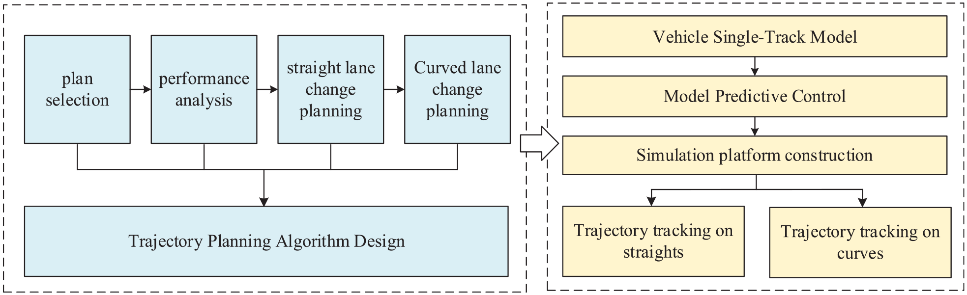
The technical route of this research.
Based on the main structure of the paper, the contributions of this paper can be summarized as follows. First, a minimum safety distance model in the longitudinal direction of the curve is proposed. Second, a lane change trajectory planning method that takes into account the adaptive correction of road curvature is established. Third, a dynamic model of the test vehicle is established and the trajectory tracking model is designed based on model predictive control. Finally, a Carsim/Simulink co-simulation model is established to verify the tracking effect of the previously established lane change trajectory.
Boundary condition of curve lane change based on longitudinal minimum safe distance model
A schematic diagram of the curve lane change scenario is shown in Figure 3. The ego vehicle M changes its lane position from the current lane to between the vehicles Ld and Fd on the target lane. Vehicles Ld, Fd, Lo, and M in the figure represent the leading vehicle in the target lane, the following vehicle in the target lane, the vehicle in front of the original lane, and the ego vehicle, respectively. It is assumed that the outer and inner lanes have the same instantaneous center, the radius of curvature of the outer lane is R, and the lane width is H.23–25 To conveniently express the relationship between the longitudinal and lateral distances between the involved vehicles, the geodetic coordinate system is shown in Figure 3, the X-axis points to the vehicle’s driving direction, and the Y-axis points to the target lane perpendicular to the X-axis. Therefore, the longitudinal acceleration, longitudinal velocity, longitudinal position, and lateral position are expressed as ai(t), vi(t), xi(t), and yi(t), respectively, where i ∈{Ld, Fd, Lo, M}. The longitudinal distance and the lateral distance represent the distance from the point P of each vehicle (the upper left corner of vehicle M in Figure 3) to the origin O of the coordinate system.26–29

The positional relationship between the ego vehicle M and the surrounding vehicles.
Longitudinal minimum safe distance model for curve lane change
The goal of this subsection is to describe how the simple curve lane change model and the longitudinal acceleration process, as described above, are used to determine the longitudinal minimum safe distance between the ego vehicle and surrounding vehicles during the time period T prior to the lane change.
(1) The longitudinal minimum safe distance between the ego vehicle M and the leading vehicle Ld in the target lane
In the curve lane change scenario shown in Figure 4, the ego vehicle M changes lanes from the outer lane to the inner lane, and there is a risk of collision between the ego vehicle M and the front vehicle
Schematic diagram of the position of the ego vehicle M and the leading vehicle
To ensure that the ego vehicle M and the leading vehicle
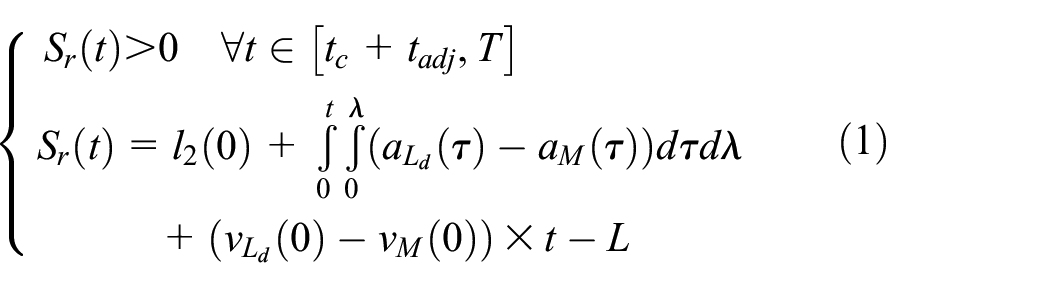
where Sr(r) refers to the longitudinal minimum safe distance between the ego vehicle M and the leading vehicle Ld in the target lane, tc denotes the initial time, tadj is the adjustment time, aLd is the acceleration of the leading vehicle, aM refers to the acceleration of the ego vehicle, vLd is the speed of the leading vehicle, and vM refers to the speed of the ego vehicle.
According to the geometric relationship, it can be determined that the calculation formulas of

It is concluded that the minimum safe distance between the ego vehicle M and the leading vehicle Ld in the target lane along the inner lane during the lane change is:

where ΔaM-Ld is the relative acceleration between the ego vehicle and the leading vehicle, and ΔvM-Ld refers to the relative speed between the ego vehicle and the leading vehicle.
According to the cosine theorem, the minimum safe distance

In the formula,
It can be seen from the abovementioned formula that the longitudinal minimum initial safety distance
(2) Longitudinal minimum safe distance between the ego vehicle
In the curve lane change scenario shown in Figure 5, the ego vehicle M changes lanes from the outer lane to the inner lane, and the collision between the ego vehicle M and the following vehicle
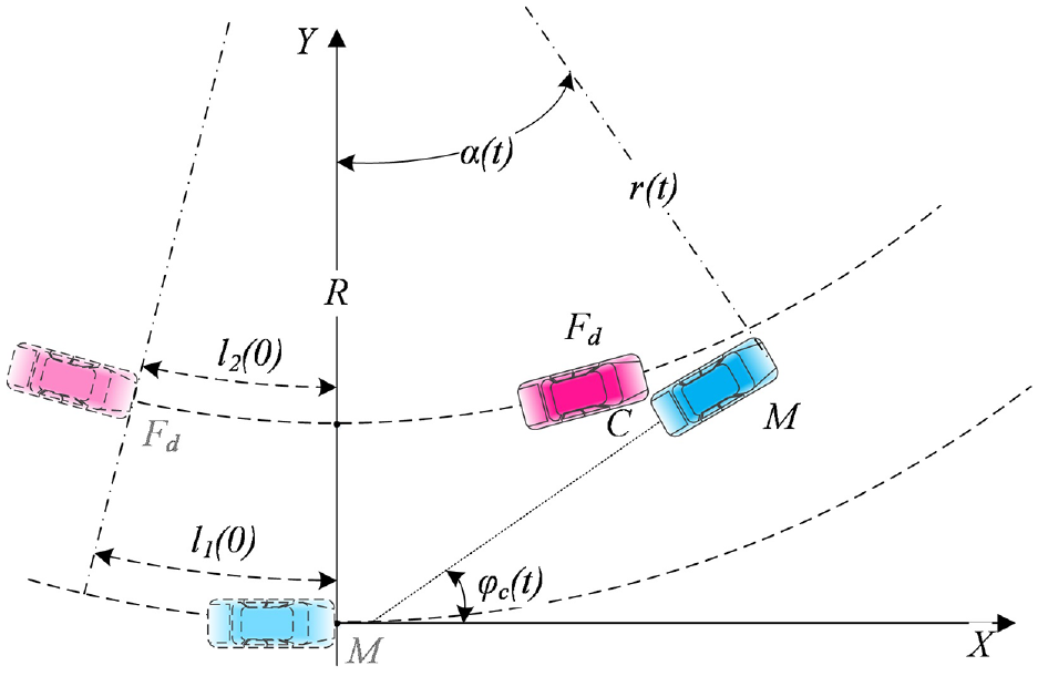
Schematic diagram of the position of the ego vehicle
To ensure that the ego vehicle M and the following vehicle
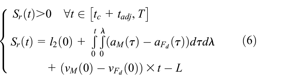
where Sr(r) refers to the longitudinal minimum safe distance between the ego vehicle M and the following vehicle Fd in the target lane, tc denotes the initial time, tadj is the adjustment time, aFd is the acceleration of the following vehicle, aM refers to the acceleration of the ego vehicle, vFd is the speed of the following vehicle, and vM refers to the speed of the ego vehicle.
According to the geometric relationship, it can be determined that the calculation formulas of

It is concluded that the minimum safe distance between the ego vehicle M and the following vehicle Fd in the target lane along the inner lane during the lane change is:

where ΔaFd-M is the relative acceleration between the following vehicle and the ego vehicle, and ΔvFd-M refers to the relative speed between the following vehicle and the ego vehicle.
When the radius of the curve tends toward infinity, it becomes a straight road, and
According to the cosine theorem, the minimum safe distance

In the formula,

It can be seen from the abovementioned formula that the longitudinal minimum initial safety distance
(3) Longitudinal minimum safe distance between the ego vehicle
In the curve lane change scenario shown in Figure 6, the ego vehicle

Schematic diagram of the position of the ego vehicle
To ensure that the ego vehicle

where Sr(r) refers to the longitudinal minimum safe distance between the ego vehicle M and the leading vehicle
It is concluded that the minimum safe distance between the ego vehicle M and the leading vehicle

where ΔaM-Lo is the relative acceleration between the ego vehicle and the leading vehicle, and ΔvM-Lo refers to the relative speed between the ego vehicle and the leading vehicle.
When the radius of the curve tends toward infinity, it becomes a straight road, and
According to the cosine theorem, the minimum safe distance

It can be seen from the abovementioned formula that the longitudinal minimum initial safety distance
Simulation verification of the minimum safe distance for changing lanes on the curved road
Simulation analysis was carried out to determine the minimum safe distance for a lane change between the ego vehicle
Figure 7 shows the relationship between the difference between the minimum safe distance and the radius of the curve when the ego vehicle

The relationship between the minimum safe distance difference and the curve radius between
Figure 8 shows the relationship between the minimum safety distance difference and the radius of the curve when the ego vehicle
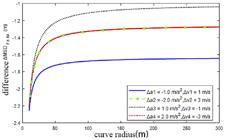
The relationship between the minimum safe distance difference and the curve radius between
Figure 9 shows the relationship between the minimum safe distance difference between the self-vehicle

The relationship between the minimum safe distance difference and the curve radius between
Lane change trajectory planning algorithm on curves
In this section, several ideal straight lane-changing trajectory algorithms are first proposed, and their advantages and disadvantages are analyzed and compared. The geometric characteristics of each trajectory are analyzed, including acceleration, velocity, position, and curvature, and are clearly described. Then the selected quintic polynomial is transformed and applied to the curved lane change trajectory with the road curvature to carry out adaptive correction, which improves the accuracy of the trajectory tracking.
Characteristic analysis of constant speed trajectory for a straight lane change
By comparing several different ideal lane-change trajectory functions, it is determined which is better for safety and comfort. The trajectory functions being compared include ramped sinusoids, quintic polynomials, and seventh-degree polynomials.
Typical lane change trajectory
Ramp sinusoids
A ramped sinusoid is characterized by continuous curvature and the rate of change. Its trajectory function is as follows:
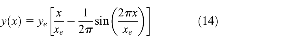
where ye and xe are the lateral and longitudinal displacements at the moment when the lane change is completed, respectively.
Quintic polynomial
A quintic polynomial is used to make the vehicle complete the lane change operation without collision within Δt time. First, the boundary conditions are defined. The initial state of the vehicle is defined as
The following trajectory functions are defined in the X and Y directions:


The time parameter matrix is defined as follows:

where


The lane change trajectory can be obtained by solving the abovementioned homogeneous linear equations. Finally, the expression in the X direction is substituted into the expression in the Y direction to obtain:

where ye and xe are the lateral and longitudinal displacements at the moment when the lane change is completed, respectively.
Seventh-degree polynomial
The seventh-degree polynomial is used to make the vehicle complete the lane change operation without collision within Δt time. First, the boundary conditions are defined as the initial state
The following trajectory functions are defined in the X and Y directions:

The time parameter matrix is defined as follows:

where

The lane change trajectory can be obtained by solving the abovementioned homogeneous linear equations. Finally, the expression in the X direction is substituted into the expression in the Y direction to obtain 30 :

where ye and xe are the lateral and longitudinal displacements at the moment when the lane change is completed, respectively (Table 1).
The ideal candidate lane change trajectory function expressions.

Figures 10 and 11 show the comparison of the candidate trajectories for lane changes in straight lanes. The lane width is set to 3.75 m, the longitudinal speed is 20 m/s, and the lane change time is 3 s. The figures show that among the three candidate trajectories, the trajectory of the fifth-order polynomial is the most gentle and smooth at the turning point, so comfort and safety are also higher.

Relationship between lateral displacement and longitudinal displacement.
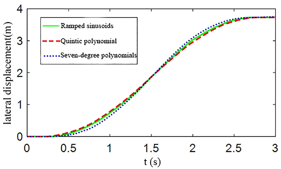
Relationship between lateral displacement and time.
Figure 12 shows a comparison of lateral speed of candidate trajectories for lane changes in straight lanes. The lane width is set to 3.75 m, the longitudinal speed is 20 m/s, and the lane change time is 3 s. The figure shows that among the three candidate trajectories, the lateral velocity of the fifth-order polynomial trajectory is the smoothest and gentlest, with the smallest peak value of about 2.2 m/s. The other two trajectories have a peak lateral speed of 2.5 m/s. Hence, the comfort and safety of the quintic polynomial are higher.

Lateral velocity comparison of candidate trajectories.
Figure 13 shows a comparison of lateral acceleration of the candidate trajectories for the straight lane change. The lane width is set to 3.75 m, the longitudinal speed is 20 m/s, and the lane change time is 3 s. The figure shows that among the three candidate trajectories, the lateral acceleration of the fifth-order polynomial trajectory is the smoothest and gentlest, with the smallest peak value of about ±2.2 m/s. The peak lateral acceleration of the other two trajectories reaches ±2.5 m/s or even exceeds ±3 m/s. Hence, the comfort and safety of the quintic polynomial are higher.

Comparison of lateral acceleration of candidate trajectories.
Figure 14 shows a comparison of the lateral acceleration rates of the candidate trajectories for lane changes on a straight road. The lane width is set to 3.75 m, the longitudinal speed is 20 m/s, and the lane change time is 3 s. The figure shows that the transition of the lateral acceleration rate of the trajectory of the fifth-order polynomial is the smoothest and gentlest among the three candidate trajectories. The other two trajectories exhibit significant fluctuations in the peak lateral acceleration rate, which can cause discomfort for the passengers during the driving experience. Hence, the comfort and safety of the quintic polynomial are higher.

Comparison of lateral acceleration rates of candidate trajectories.
Figure 15 shows a comparison of the yaw angle of three candidate trajectories for a straight lane change. The lane width is 3.75 m, the longitudinal speed is 20 m/s, and the lane change time is 3 s. The figure shows that among the three candidate trajectories, the transition of the yaw angle of the quintic polynomial is the gentlest and smoothest, with the smallest peak value. The peaks of the other two yaw angles are relatively sharp, which can cause discomfort for passengers during the driving experience. Hence, the comfort and safety of the quintic polynomial are higher.

Comparison of yaw angles of candidate trajectories.
Figures 16 and 17 show the comparison of the candidate trajectory curvature and front wheel turning angle for the same straight lane change, respectively. The lane width is 3.75 m, the longitudinal speed is 20 m/s, and the lane change time is 3 s. The figure shows that among the three candidate trajectories, the quintic polynomial is the gentlest and smoothest at the transition, resulting in higher comfort and safety.
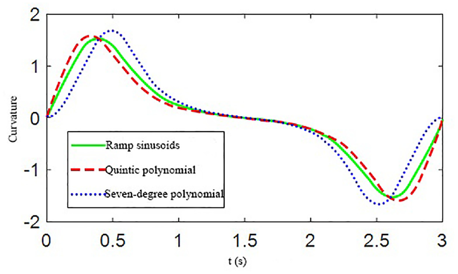
Curvature comparison of candidate trajectories.

Comparison of front wheel rotation angles of candidate trajectories.
Curve lane change trajectory correction
The planning and research for the trajectory of a lane change on a straight road have been conducted before. However, ensuring that lane changes are straight when transitioning between curved lanes is challenging.31,32 Therefore, there is a need to carry out further research and discussions on trajectory planning for the lane changes on curved roads. The following is a discussion on planning a curved lane change trajectory based on the trajectory planning for a straight lane change, mainly including the lane changes from the outer lane to the inner lane and from the inner lane to the outer lane.
Analysis of vehicle status in curved lane change
Lane change from outer lane to inner lane
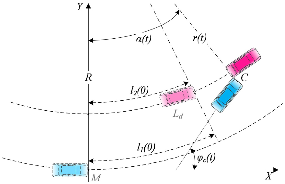
A schematic diagram of a lane change from the outer lane to the inner lane is shown in Figure 18, where OXY is the geodetic coordinate system, and the two dashed lines are the lane center lines, which have the same instantaneous center. The radius of the outer lane centerline is R, the lane width is H, and point C is any point on the lane change trajectory.

Schematic diagram of lane change from outer lane to inner lane.
When the vehicle changes lanes from the outer lane to the inner lane, the distance the vehicle moves along the instantaneous radius to the instantaneous center of rotation is

The instantaneous radius of the position of the center of mass of the vehicle is:

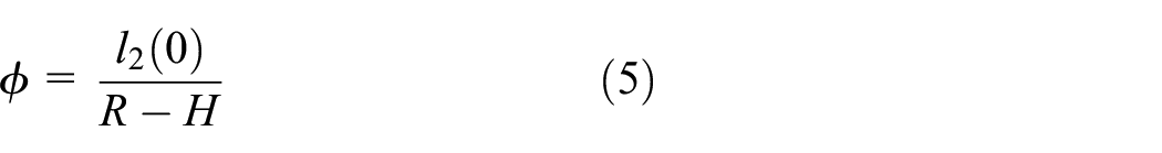
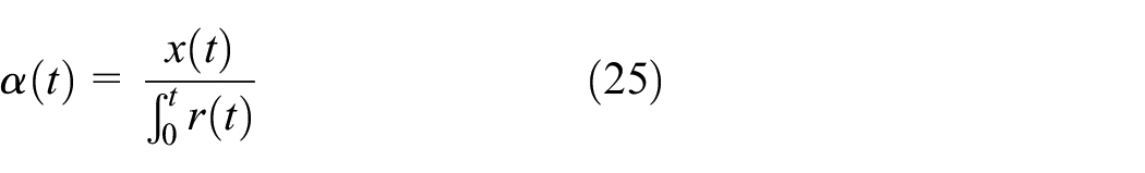
The angle that the vehicle’s center of mass rotates around the instantaneous center of rotation is:
By solving the first derivative and the second derivative of the abovementioned formula, the angular velocity and angular acceleration can be obtained:


Thus, the yaw angle, yaw angular velocity, and yaw angular acceleration are obtained when the vehicle lane changes:

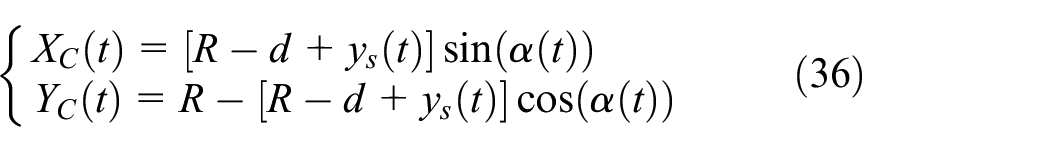
In summary, it can be calculated that the coordinates of the center of mass in the geodetic coordinate system when the vehicle turns lanes are changed as:

Lane change from inner lane to outer lane
A schematic diagram of the lane change from the inner lane to the outer lane is shown in Figure 19, where OXY is the geodetic coordinate system and the two dashed lines are the lane center lines, which have the same instantaneous center. The radius of the outer lane centerline is R, the lane width is H, and point C is any point on the lane change trajectory.

Schematic diagram of lane change from the inner lane to the outer lane.
When the vehicle changes lanes from the outer lane to the inner lane, the distance the vehicle moves away from the instantaneous center of rotation along the instantaneous radius is:

The instantaneous radius of the position of the center of mass of the vehicle is:

The angle that the vehicle’s center of mass rotates around the instantaneous center of rotation is:

By solving the first derivative and the second derivative of the abovementioned formula, the angular velocity and angular acceleration can be obtained:


Thus, the yaw angle, yaw angular velocity, and yaw angular acceleration when the vehicle lane changes are obtained:

In summary, the coordinates of the center of mass in the geodetic coordinate system when the vehicle changes lanes on a curve can be calculated as:
Trajectory simulation of curve lane change
According to the research on trajectory planning for acceleration lane changes on straight roads, the planning of the lane change trajectory in the curve acceleration is established. The simulation parameters are set as follows. It is assumed that the lane width is 3.75 m, the outer lane radius is 1500 m, the inner lane radius is 1500–3.75 m, the lane change time is 3 s, the vehicle longitudinal speed is 20 m/s, and the vehicle longitudinal acceleration is 2 m/s2. The simulation results are shown in Figures 20 to 28.

Comparison of acceleration/constant speed trajectories from the inner lane to the outer lane.

Comparison of acceleration/constant speed lateral accelerations from the outer lane to the inner lane.

Comparison of acceleration/constant speed lateral accelerations from the inner lane to the outer lane.

Comparison of acceleration/constant jerks from the outer lane to the inner lane.

Comparison of acceleration/constant jerks from the inner lane to the outer lane.

Comparison of front wheel turning angle from the outer lane to the inner lane with acceleration/constant speed.
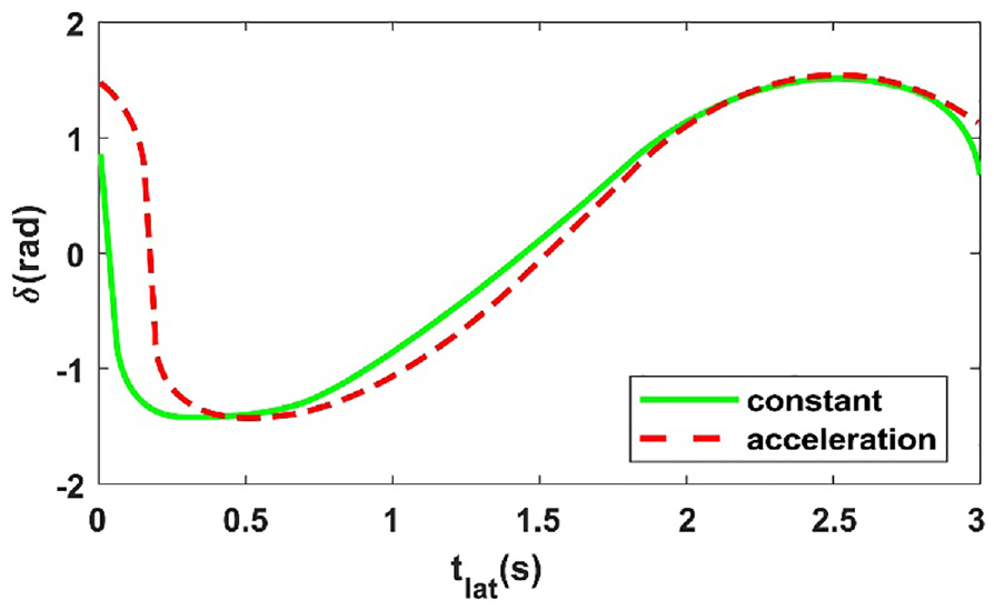
Comparison of front wheel turning angle from the inner lane to the outer lane with acceleration/constant speed.

Curvature comparison of constant speed trajectories from the outer lane to the inner lane.

Curvature comparison of acceleration/constant speed trajectories from the inner lane to the outer lane.
Model predictive control
The vehicle dynamics model plays an important role enabling the vehicle to follow the planned trajectory. First, by transforming the equivalent constraints of complex dynamic models, the amount of computation can be reduced, and real-time performance of the system can be improved in planning and control. Second, the MPC algorithm can take into account multiple control objectives of the system while imposing control constraints, so as to ensure the stability of the control system and realize the optimization of the system. The purpose is to enable the vehicle to effectively follow the target trajectory when actively changing lanes. Therefore, using an accurate dynamic model in model predictive control can improve the following ability of the system and allow for full use of the driving performance of the vehicle, such as avoiding obstacles in high-speed conditions.33–36
In low-speed driving conditions, the kinematic constraints have a greater impact on the vehicle, whereas dynamic constraints have less impact. As the speed increases, the role of dynamic constraints is highlighted and model predictive control is used for control with constraints.37–39 Therefore, model predictive control is used to control and track the planned lane change trajectory described in the previous section.
Dynamic modeling based on vehicle single-track model
The research goal of this study is to enable a vehicle to track the planned trajectory in real time and stably. For this, the vehicle tire model is used to analyze the vehicle tracking characteristics. Moreover, the model predictive control is used to track the trajectory, and the vehicle dynamics model can be simplified appropriately to ensure maximum accuracy. This can reduce the amount of calculation required during the operation of the control algorithm improving the real-time tracking. 40
In summary, this research makes the following assumptions about the vehicle dynamics model:
The vehicle is driven on a smooth road without obvious potholes, ignoring vertical motion.
The effect of suspension motion is not considered; that is, the vehicle is assumed to be rigid.
During vehicle motion, aerodynamic effects during longitudinal and lateral motion are not considered.
The monorail model replaces the vehicle model. That is, when the vehicle turns, it is assumed that the steering angles of the left and right wheels are the same and the influence of the left and right transfer of the load on the movement process is ignored.
The cornering stiffness remains unchanged during vehicle motion.
Based on the abovementioned assumptions, the vehicle is assumed to have a front-drive, and the plane motion of the vehicle has only three degrees of freedom, namely longitudinal, lateral, and yaw motion. The vehicle monorail model is shown in Figure 29. In the figure,
Using Newton’s second law, which states that the external force on an object is equal to the product of its mass and its acceleration, the force balance equations along the

Vehicle monorail model.
In the x-axis direction, there is:

In the y-axis direction, there is:

In the direction around the z-axis, there is:

In the formula,
The functional relationships between the resultant forces


Since the longitudinal force and lateral force of each tire of the vehicle are related to the slip rate, road adhesion coefficient, vertical load, and tire slip angle, the following expressions can be obtained:


where
The tire side slip angle can be calculated with the following formula under the vehicle coordinate system:

In the formula,


where
In practice, the speed of vehicle tires often needs to be obtained indirectly:


Normally, the slip ratio between the tire and the road surface is calculated with the following formula:
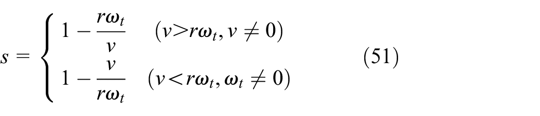
where
Without considering the load transfer of the front and rear axles of the vehicle, the vertical loads of the front and rear axles can be calculated with the following formula:


In summary, the nonlinear dynamic model of the vehicle can be obtained. All parameters, except for the tire slip rate and the road adhesion coefficient, can be calculated from the state parameters of the vehicle. The pavement adhesion coefficient is an inherent parameter of the pavement, which can be generally obtained under the given pavement conditions. The tire slip rate itself is a very complex issue. Usually, a vehicle is equipped with a good ABS system, and the slip rate is always maintained at the optimal working point. Therefore, the following expression can be obtained:
In the abovementioned formula, the state quantity is
Under normal driving conditions, the vehicle tire slip angle and its slip rate are small, so the tire force can be assumed to be a linear equation. Specifically, in the case of lateral acceleration.

where
There are many trigonometric functions in the vehicle dynamics model proposed in the previous section, which is not conducive to calculation and solution, so this section adopts the small angle assumptions as follows:

The calculation formula of the tire side slip angle can be obtained with the joint solution of the abovementioned formulas, as follows:

According to the abovementioned formula, the longitudinal force a and lateral force b of each tire of the vehicle are calculated and solved as follows:


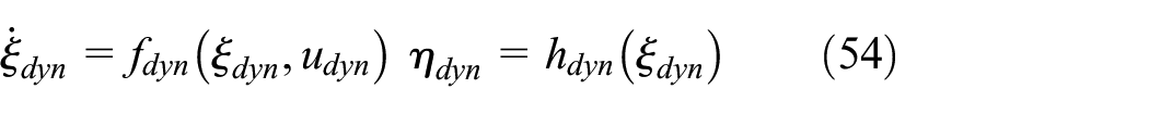
The simplified nonlinear model of vehicle dynamics is given as follows:


In this system, the state quantity is
Model predictive controller design
Linearization of nonlinear dynamic models
For the nonlinear dynamic model established as described in the previous section,
The nonlinear dynamic model is linearized according to the deviation between the expected trajectory of the lane change and the actual driving state quantity of the vehicle, and the following equation is obtained:
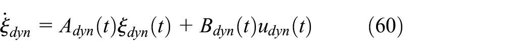
where
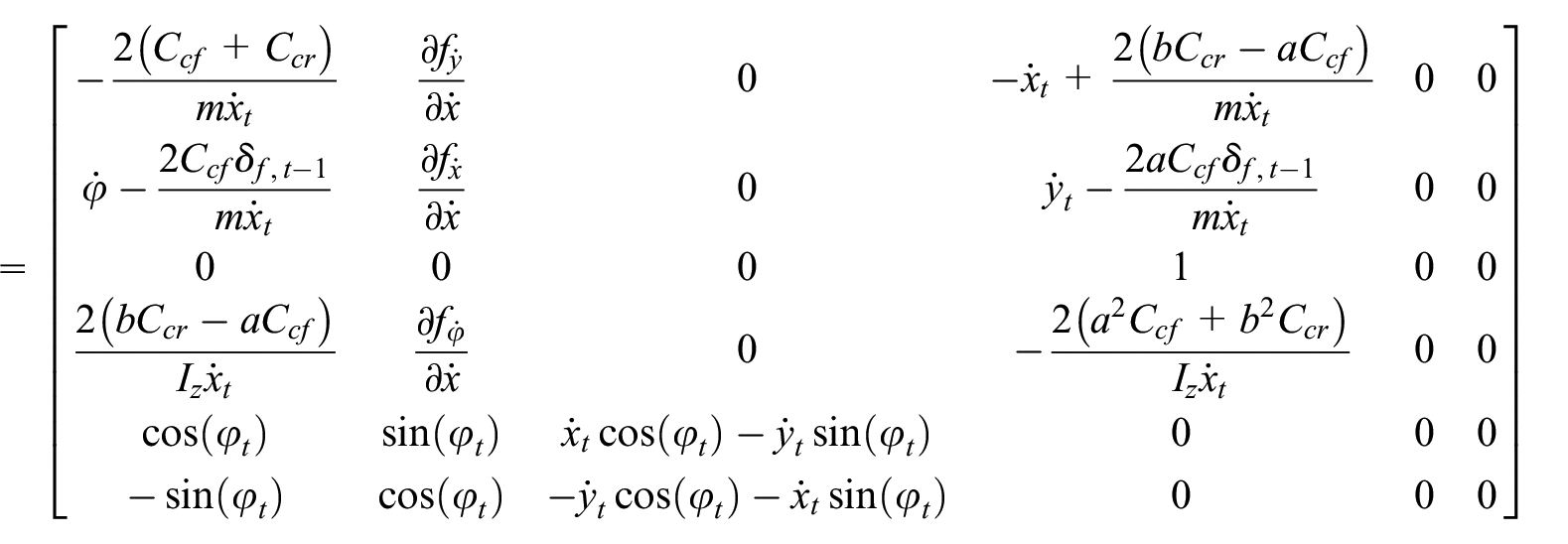
In the abovementioned formula,

The abovementioned linear dynamic model is discretized by the first-order difference quotient:

Where
Controller constraints
(1) The speed constraints during the driving process of the vehicle are as follows:

In the formula,
(2) The front wheel turning angle constraints during the driving process of the vehicle are as follows:

(3) The constraints on the side-slip angle of the center of mass during vehicle driving are as follows:


(4) The lateral acceleration constraints during vehicle driving are as follows:

(5) The tire slip angle constraints during vehicle driving are as follows:

Controller objective function
Due to the complexity of the dynamic model, for the choice of an objective function without a relaxation factor, there is a high probability that the optimal solution or sub-optimal solution cannot be obtained within a given time interval. Therefore, the objective function with the relaxation factor is used in this research, and the expression is as follows:

Combining the constraint assumptions discussed in the previous subsection and the objective function given in this subsection, the vehicle lane change trajectory tracking problem based on model predictive control is transformed into an optimization problem, as follows:

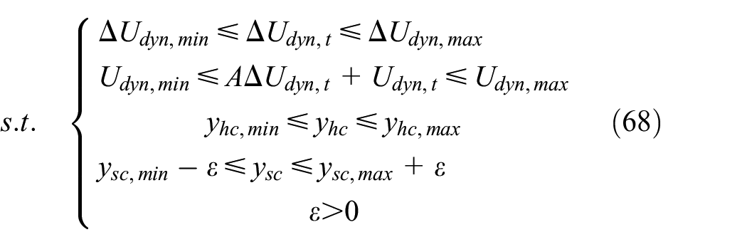
In the formula,
After completing the solution of the abovementioned equation in each cycle, a series of control inputs is obtained:

Each time, the first element in the control sequence is applied to the control system:

After entering the next control cycle, the abovementioned process is iterated. The tracking of the lane change trajectory can be completed in this way.
Lane change trajectory tracking simulation
Using the CarSim vehicle dynamics simulation platform and the PreScan vehicle dynamic scenario establishment platform, a lane change trajectory tracking model is established in Matlab/Simulink based on model predictive control. The model includes vehicle dynamics parameters, simulation conditions, relative position information of this vehicle and adjacent vehicle, initial motion state, and simulated road conditions. These parameters are shown in Tables 2 and 3. The input and output interfaces of the CarSim vehicle dynamics model are defined to achieve data transmission between the Matlab/Simulink control strategy model and the CarSim vehicle dynamics model. The output signal of the ego vehicle includes position information, lateral velocity, longitudinal velocity, lateral acceleration, and yaw angle information, while the ego vehicle input signal includes external sensor information, initial speed, and steering wheel angle.
Vehicle parameters.

Testing parameter.

Figure 30 shows the lane change trajectory tracking control strategy model built in the Matlab/Simulink environment. The simulation model on the CarSim/PreScan/Simulink co-simulation platform is built based on the previously designed lane change decision conditions, trajectory model, and trajectory tracking model based on model predictive control. The results of the simulation demonstrate the trajectory tracking effect, as shown in Figures 31 to 33.

Lane change trajectory tracking model.

Comparison of the expected Y versus X trajectory and the actual Y versus X trajectory of the lane change on the straight.

Comparison of expected trajectory and actual trajectory of curved lane change.

The difference between the expected trajectory and the actual trajectory of the curved lane change.
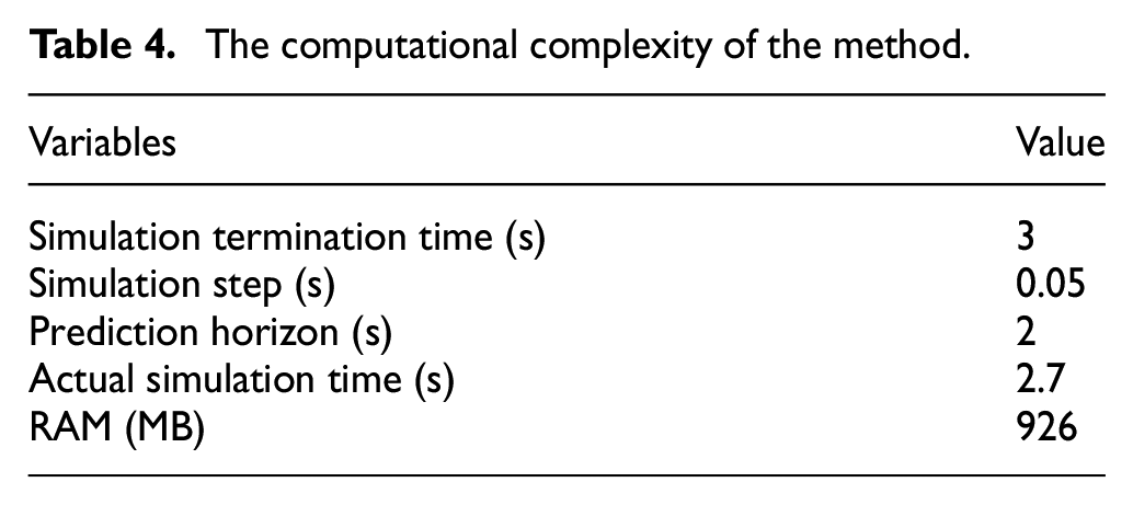
The real-time verification of the algorithm is shown in Table 4. The simulation is terminated at 3 s, the simulation step is set to 0.05 s, and the prediction horizon (s) is 2 s. The system takes 2.7 s to run, and the RAM used is 926 MB, which is suitable for real-time applications in engineering, as confirmed by MATLAB.
The computational complexity of the method.
Conclusions
This research focuses on the study and analysis of curve trajectory planning and trajectory tracking in lane change.
The trajectory planning for a lane change with a certain curvature is analyzed, including the lane change trajectory planning and the minimum safe distance model in the cases of straight and curved roads. When the curvature of the curve is relatively small, there is little difference between using the straight lane change minimum safe distance model/trajectory model or the curved lane change minimum safe distance model/trajectory model. However, when the curvature of the curve is large, the gap between the minimum safe distance models for straight and curved lane changes becomes more noticeable.
The trajectory tracking control strategy for model predictive control based on the rolling optimization idea is designed. In this paper, model predictive control based on the idea of rolling optimization is selected for trajectory tracking. In addition to being suitable for multi-input and multi-output nonlinear models, model predictive control also has the advantage of considering the model’s constraints. Therefore, the obtained control amount is more consistent with the vehicle dynamics characteristics, resulting in more accurate trajectory tracking results.
Footnotes
Handling Editor: Chenhui Liang
Declaration of conflicting interests
The author(s) declared no potential conflicts of interest with respect to the research, authorship, and/or publication of this article.
Funding
The author(s) disclosed receipt of the following financial support for the research, authorship, and/or publication of this article: This research was funded by the Scientific research project of CATARC Automotive Test Center (Tianjin) Co., Ltd, grant number TJKY2223039 and by the Science and Technology Planning Project of Jilin, China, grant number 20210301023GX.