Nonlinear model predictive control for trajectory tracking of nonholonomic mobile robots

Abstract

Trajectory tracking for autonomous vehicles is usually solved by designing control laws that make the vehicles track predetermined feasible trajectories based on the trajectory error. This type of approach suffers from the drawback that usually the vehicle dynamics exhibits complex nonlinear terms and significant uncertainties. Toward solving this problem, this work proposes a novel approach in trajectory tracking control for nonholonomic mobile robots. We use a nonlinear model predictive controller to track a given trajectory. The novelty is introduced by using a set of modifications in the robot model, cost function, and optimizer aiming to minimize the steady-state error rapidly. Results of simulations and experiments with real robots are presented and discussed verifying and validating the applicability of the proposed approach in nonholonomic mobile robots.

Introduction

This article proposes a nonlinear model predictive controller. approach to solve the trajectory tracking problem (TTP) of a nonholonomic wheeled mobile robot. One of the first surveys dealing with the nonholonomic control problems is provided by Kolmanovsky and McClamroch. ¹ In the survey, the authors mention two problems (motion planning control systems and feedback stabilization) and point out three other important issues: models of nonholonomic control systems, new control approaches for motion planning of nonholonomic systems and stabilization of these new approaches. Nonetheless, new approaches in optimal control arise after that. ^2,3 One of these introduced approaches is the model predictive control (MPC). The MPC problem has its origin in the late 1970s and has being developed considerably since then. ⁴ According to Findeisen and Allgöwer, ⁵ the MPC problem is formulated as solving, online, a finite horizon open loop optimal control problem subject to system dynamics and constraints involving states and controls.

TTPs for autonomous vehicles are usually solved by designing control laws that make the vehicles track predetermined feasible trajectories by way of minimizing the trajectory error that is the difference between the robot pose and the trajectory coordinates. ⁶ However, this approach suffers from the drawback that usually the vehicle dynamics exhibit complex nonlinear terms and significant uncertainties, specially when nonholonomicity is present. The controller attempts to make the outputs catch up with the time-parameterized desired outputs. This may lead to closed loop performance difficulties and too large control signals. ⁷ In contrast, one can argue that we can counter this problem by more complex modeling in classic NMPC or by using robust NMPC. More complex modeling brings up the increase in computational cost ⁸ while robust approaches usually use learning-based approaches either increases the computational cost or need a off-line training phase. ⁹ Some works on nonlinear path following control in robotics have been proposed ^{10 –13} using other approaches. To deal with the above difficulties, here we propose a nonlinear model predictive control (NMPC) to solve the TTP and increase the controller accuracy by considering each position of the given global path as a position of a virtual target to be pursued. This has led us to modify the classic NMPC controller applied to the TTP.

Therefore, our main contribution is to propose a NMPC that uses a modified cost function to minimize the distance between the robot pose and the given global trajectory coordinate, and minimize the difference between the robot orientation and the orientation acquired from the vector of the distance between the robot pose and the reference coordinate, instead of tracking the error in the robot’s pose regarding the predicted coordinates given by the path generator subblock. These modifications can be observed in Figure 1, which will be detailed furthermore. As a consequence, we do not use a path generator subblock for the prediction horizon in the NMPC. As a result, it increases the nonlinearity of the system. To maintain the stabilization of the steady state of the system, we use the 1-norm in the control effort term of the modified cost function. To better handle these nonlinearities, we use the Resilient Propagation (RPROP) algorithm to minimize the cost function. ¹⁴ With all of these modifications, our proposal is able to perform the control in a desirable way. Some recent approaches also use the concept of a virtual leader. ^15,16 Although they differ from our approach in numerous parts, it is interesting to note that they confirm that approaches not error dependent are beginning to become more studied due to its better results with respect to classical NMPC.

Figure 1.

Classical NMPC approach (left) and our approach (right).

Classic nonlinear model predictive controller for trajectory tracking

Many researchers have used NMPC to solve the trajectory tracking control problem of nonholonomic mobile robots. ^{17 –19} The NMPC’s ability to enable a robot to track a trajectory is due to the fact that the cost functions used by the controller minimize a deviation of the predicted behavior of the robot. The minimization by the optimizer and the predicted behavior are the main blocks of the MPC theory. When applied to solve the trajectory tracking control problem, the NMPC usually is divided into three subblocks:

Path generator: This subblock receives the global trajectory calculated by a trajectory generator and creates a reference signal to be followed by the controller in a given prediction horizon;

Optimizer: This subblock uses an online numeric minimization method to optimize the cost function and generate the optimal inputs; MPC usually uses the gradient descent algorithm when applied to mobile robotics; and

Predictor: The predictor computes the predicted state evolution of the robot itself; it uses a simplified robot model to emulate the robot’s evolution and calculate the final value of the cost function.

Since linear (and even successively linearized or time-variant) MPC is not feasible for this mechanical benchmark problem (as linearizing around any fixed point is not controllable and the assumptions for guaranteed stability do not hold), the potential of nonlinear model predictive control (NMPC) techniques is investigated over the years. ^20,21 In contrast, NMPC implementations demonstrated that the expense and reliability of the nonconvex optimization causes problems, causing the tuning process of the controller parameters to be decisive. In general, terminal state constraints are required to guarantee asymptotic stability. ²²

Regarding the optimizer subblock, the work of Vougioukas ²³ presents a nonlinear model predictive controller for mobile robots. The basic idea is to use a motion model for the vehicle and compute in real time an optimal M-step-ahead control sequence, which minimizes the total M + 1 step tracking error of the projected motion. In the presence of obstacles, the controller deviates from the reference trajectory by incorporating into the optimization obstacle-distance information from range sensors. In 2008, Lim et al. ¹⁷ presented a practical approach for a nonlinear model predictive control scheme with collision avoidance which is implemented on a mobile robot with two differential wheels. The optimal control input was solved by a discrete nonlinear optimization problem over a predescribed prediction horizon based on a gradient descent method using Lagrange multipliers. Two years later, Pan and Wang ²⁴ presented a recurrent neural network (RNN) approach to nonlinear model predictive control (NMPC). By using decomposition, the original optimization associated with nonlinear MPC was reformulated as a quadratic programming problem with unknown parameters. They employed an RNN and developed a learning algorithm for solving the formulated problem.

To overcome the online optimization issue and to ensure asymptotic convergence of the tracking error, Hedjar et al. ²⁵ used Taylor series approximation in the prediction model. As the years have passed, computational power increased and several researches performed experiments with more complex robot models such as car trailer. ^26,27 Recently, obstacle avoidance has also being a topic of research in nonlinear MPC with nonholonomic robots or omnidirectional robots. ^7,26,28

When analyzing the predictor subblock, a simple prediction model means less computational cost and less precision in prediction. According to Figure 1, the relevant variables for the kinematic model of a typical two-wheel differential mobile robot are its center position coordinates ( $x_r,y_r$ ), its angle of orientation θ_r, along with its linear and angular velocities $(v_r,{\omega }_r)$ , respectively. Therefore, the classic prediction model derived from the diagram presented in Figure 1 results in the prediction model described in equation (1). The constraint shown in equation (2) must be respected in order to avoid lateral spilling from the wheels described by

$\left[\begin{array}{c}\dot{x}\\ \dot{y}\\ \dot{\theta }\end{array}\right]=\left[\begin{array}{cc}\text{cos}\theta & 0\\ \text{sin}\theta & 0\\ 0& 1\end{array}\right]\mathrm{.}\left[\begin{array}{c}v\\ \omega \end{array}\right]$

1

and

$\dot{x}\text{sin}\theta -\dot{y}\text{cos}\theta =0$

2

Finally, we can perceive the error states ( $x_e,y_e,{\theta }_e$ ) used to predict the robot’s movement error, which are selected in a rotated coordinate frame and presented in the work by Gu and Hu, ²⁹ as follows

$\left[\begin{array}{c}{x}_e\\ y_e\\ {\theta }_e\end{array}\right]=\left[\begin{array}{ccc}\text{cos}\theta & \text{sin}\theta & 0\\ -\text{sin}\theta & \text{cos}\theta & 0\\ 0& 0& 1\end{array}\right]\left[\begin{array}{c}{x}_{\text{ref}}-x\\ y_{\text{ref}}-y\\ {\theta }_{\text{ref}}-\theta \end{array}\right]$

3

where a desired reference trajectory is defined by a reference state vector $X_{\text{ref}}=[x_{\text{ref}}{y}_{\text{ref}}{\theta }_{\text{ref}}{]}^{\text{T}}$ .

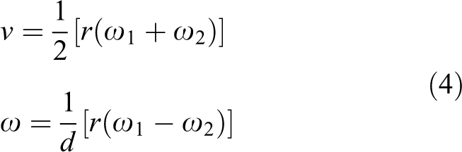
Now, we need to explicit the relation between linear and angular velocities (v and ω) with the wheel motion. The relation between the angular velocity of each wheel and the robot’s linear and angular velocities is shown in equation (4), where ω₁ and ω₂ are the angular velocities of the right and left wheels, respectively, r is the wheel radius, and d is the length of the robot base (distance between both wheels). Therefore

$\begin{array}{l}v=\frac{1}{2}[r({\omega }_1+{\omega }_2)]\hfill \\ \omega =\frac{1}{d}[r({\omega }_1-{\omega }_2)]\hfill \end{array}$

4

By combining equations (1) and (4), we can obtain a model that expresses the robot’s coordinates and orientation in terms of the angular velocity output by its wheels, as can be seen in equation (5), where

$\left[\begin{array}{c}\dot{x}\\ \dot{y}\\ \dot{\theta }\end{array}\right]=\left[\begin{array}{cc}\frac{r\text{cos}\theta }{2}& \frac{r\text{cos}\theta }{2}\\ \frac{r\text{sin}\theta }{2}& \frac{r\text{sin}\theta }{2}\\ \frac{r}{d}& \frac{-r}{d}\end{array}\right]\left[\begin{array}{c}{\omega }_1\\ {\omega }_2\end{array}\right]$

5

Also, equation (4) can be easily manipulated to show the direct relation between the control input (the linear and angular velocities corresponding to the desired trajectory) and the output (the right and left wheels’ angular velocities). This is shown in equation (6)

$\begin{array}{l}{\omega }_1=\frac{1}{r}\left(v+\frac{\omega d}{2}\right)\hfill \\ {\omega }_2=\frac{1}{r}\left(v-\frac{\omega d}{2}\right)\hfill \end{array}$

6

In most cases, specially in simulations, the kinematic model of the robot used in the predictor is sufficient to maintain a small tracking error by the MPC/NMPC. Nevertheless, in real robot systems, this model does not suffice. Dead zone, saturation, friction, slippery, uncertainties arisen from parameter variations or from neglected dynamics, and nonholonomicity are examples of nonlinearities that are difficult to model and when it can be modeled, it increases the computational cost of the predictive controller. ³⁰

One way to perform such prediction with high precision and low computational cost is by using neural models such as neural networks. ³¹ The article by Gomez-Ortega and Camacho ³² presented a way of implementing a MPC for mobile robot path tracking using a nonlinear model of mobile robot dynamics and thus allows an accurate prediction of the future trajectories. In 2007, Conceição et al. ³³ presented a nonlinear model-based predictive controller (NMPC) for trajectory tracking of a mobile robot. Methods of numerical optimization to perform real-time nonlinear minimization of the cost function were used and the cost function penalized the robot position error, the robot orientation angle error, and the control effort. Their approach was then improved considering friction in the dynamic model for friction compensation. ³⁴

Finally, in recent researches, stabilization of nonholonomic systems has been studied. ²¹ One of the last NMPC works discussed on providing optimization-based solutions to the state estimation and tracking control problems in mobile robotics, specially in nonholonomic robotic systems. The work by Jayasiri et al. ³⁵ proposed to solve the estimation problem by using moving horizon estimation approach while using a nonlinear model predictive control (NMPC) for solving the tracking control problem.

In all above-mentioned works, a NMPC’s cost function, when applied to the trajectory tracking of a differential mobile robot, is such as follows

$\begin{array}{ll}J({\widehat{R}}_p,U)\hfill & ={\displaystyle \sum _{i=N_1}^{N_p}}{\lambda }_1\times ([x(k+i)-x_{\text{ref}}(k+i{)]}^2\hfill \\ \hspace{0.17em}\hfill & \hspace{1em}\hspace{1em}\hspace{1em}\hspace{1em}\hspace{1em}+{[y(k+i)-y_{\text{ref}}(k+i)]}^2)\hfill \\ \hspace{0.17em}\hfill & \hspace{1em}+{\displaystyle \sum _{i=N_1}^{N_p}}{\lambda }_2\times {(\theta (k+i)-{\theta }_{\text{ref}}(k+i))}^2\hfill \\ \hspace{0.17em}\hfill & \hspace{1em}+{\displaystyle \sum _{i=1}^{N_c}}{\lambda }_3\times {(\Delta U(k+i-1))}^2\hfill \end{array}$

7

where ${\widehat{R}}_p={\left[\begin{array}{ccc}x& y& \theta \end{array}\right]}^{\text{T}}$ is the predicted state of the robot. N₁ and N_p are the prediction horizon limits in discrete time, such that N₁ > 0 and N_p ≤ 8. N_c = 2 is the control horizon. λ₁, λ₂, and λ₃ are the weights for each component of the cost function. $\Delta U(k+i-1)$ is the variation of the control signals, where U is the output control signal from the optimizer sent to the predictor.

This cost function of the NMPC represents the cost to be minimized by the predictive controller. It is typically associated with the dynamical change of the system over time. When applied to minimizing the error in the TTP of mobile robots, this cost function is usually minimized by a classical gradient descent optimization method. In the TTP, the cost function must penalize the difference between the pose of the robot and the pose of reference given by the trajectory generator. Additionally, the cost function has a term that penalizes the control effort. Each of the penalization is associated with a weight that defines the proportion of penalization on the global value of the cost function.

As above mentioned, classical methods ^{7,17,18,25,28,29} usually use a path generator block to create a path within the prediction horizon. This approach creates a need for the correct modeling of the generated path. In contrast, our approach does not need this block. Furthermore, the cost function we propose is not formulated in the quadratic form but using the 1-norm. This approach increases the nonlinearity of the controller, which in turn can handle the nonlinearities present on the controlled system. ⁴

A novel nonlinear model predictive controller approach

We now present an approach for nonlinear model predictive control when applied to nonholonomic trajectory tracking of mobile robots. The proposed control approach can achieve better results in trajectory tracking control of mobile robots than classical control approaches. We assume that each position and velocity given by the trajectory generator is the state of a virtual target to be tracked. In turn, it generates a set of modifications on the NMPC classical approach that improves it in such fashion that it increases the controller’s accuracy and the controller’s nonlinearities, that is, we can apply the same cost function weights in different types of trajectory with low steady-state error without the need of retuning the controller gains. With this assumption, we can track the desired coordinates penalizing undesired behaviors.

As above observed, the classical NMPC approach ^29,36 has a subblock to generate a path from the robot’s current point to the N_p-ahead points in order to better track the trajectory error. Taking into account that the position given by the global trajectory generator is a virtual leader position, this subblock loses its importance. Therefore, in our approach, the NMPC is divided into only two subblocks:

Optimizer: We use here the RPROP algorithm by Riedmiller and Braun ¹⁴ ;

Predictor: Kinematic robot model and modified cost function.

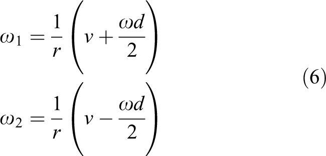
Figure 2 illustrates the structure of the proposed NMPC uses, where $U(k|k)=U_{\text{best}}(k)={\left[\begin{array}{cc}{v}_{\text{best}}(k)& w_{\text{best}}(k)\end{array}\right]}^{\text{T}}$ is the output control signal, $\widehat{U}(k+i|k)$ with $i=\mathrm{0...}{N}_c-1$ , or simply U, is the output control signal from the optimizer sent to the predictor, and $\widehat{J}(k+i|k)$ with $i=\mathrm{1...}{N}_p$ , or simply J, is the response of the predictor block to each $\widehat{U}(k+i|k)$ . Here, at an instant k, the robot sends its pose $Ro{b}_{\text{state}}(k)={\left[\begin{array}{ccccc}x(k)& y(k)& \theta (k)& v(k)& \omega (k)\end{array}\right]}^{\text{T}}$ to the NMPC to be used by the predictor subblock. Our NMPC also receives the position of the virtual target (position given by the trajectory generator) in the world frame $P_{\text{t}}(k)={\left[\begin{array}{cc}{x}_{\text{ref}}(k)& y_{\text{ref}}(k)\end{array}\right]}^{\text{T}}$ and the velocity of the virtual target (velocity given by the trajectory generator) in the world frame $V_{\text{t}}(k)={\left[\begin{array}{cc}{v}_x{\hspace{0.17em}}_{\text{ref}}(k)& v_y{\hspace{0.17em}}_{\text{ref}}(k)\end{array}\right]}^{\text{T}}$ .

Figure 2.

Controller diagram.

After receiving the states of the robot and the virtual target, the controller’s optimizer subblock provides the control input $\widehat{U}(k+i|k)$ , in a limited control horizon, to the predictor subblock, which then predicts the robot state ( ${\widehat{R}}_p$ ) evolution for N_p steps (prediction horizons) through the prediction model (MOD block in Figure 2), and provides a cost value through the cost function (F.C. block in Figure 2) to the optimizer $\widehat{J}(k+i|k)$ in accordance with $\widehat{U}(k+i|k)$ . The iterative minimization process is repeated in cyclic fashion. Finally, the control output in the first step $U_{\text{best}}(k)$ is sent to the robot. To achieve cost function minimization, the NMPC’s predictor subblock estimates the evolution of the robot behavior, as well as the behavior of the target which is used by the NMPC’s optimizer and predictor subblocks for the cyclic minimization process. After processing the control calculations, the NMPC sends the desired control output back to the robot (controller’s reference velocities).

The model

As mentioned above, we need to change the prediction model in order to take the global trajectory given positions and velocities as if they were the positions and velocities of a virtual leader to be followed. Therefore, we start our model by using the same equations from the classic prediction model seen in equations (1) to (6), except for equation (3).

The nonholonomic mobile robot model used in the predictor is a nonlinear simplified model that, when properly parameterized, is advantageous in order to reduce the computational load of each cycle of the control algorithm. The model is initialized with motor velocity limitation by detecting saturation and proportionally scaling the other motors velocities that can be seen as an input constraint. ³³ The robot state ( $({\text{Rob}}_{\text{state}}(k))$ ) containing the pose and velocity is defined as

${\text{Rob}}_{\text{state}}(k)={\left[\begin{array}{ccccc}x(k)& y(k)& \theta (k)& v(k)& \omega (k)\end{array}\right]}^{\text{T}}$

8

and the simulation of the state evolution ( ${\widehat{R}}_p$ ) is given by

$\left[\begin{array}{c}x(k)\\ y(k)\\ \theta (k)\end{array}\right]=\left[\begin{array}{c}x(k-1)\\ y(k-1)\\ \theta (k-1)\end{array}\right]+\tau \mathrm{.}\left[\begin{array}{c}\dot{x}(k)\\ \dot{y}(k)\\ \dot{\theta }(k)\end{array}\right]$

with τ as the time step and ${[\dot{x}(k)\dot{y}(k)\dot{\theta }(k)]}^{\text{T}}$ being found through equation (1).

Taking into account the presented elements, the position P_t(k) and velocity V_t(k) of the virtual target (trajectory given positions and velocities) in the world frame at an instant k are defined as

$\begin{array}{l}{P}_{\text{t}}(k)={\left[\begin{array}{cc}{x}_{\text{ref}}(k)& y_{\text{ref}}(k)\end{array}\right]}^{\text{T}}\hfill \\ V_{\text{t}}(k)={\left[\begin{array}{cc}{v}_x{\hspace{0.17em}}_{\text{ref}}(k)& v_y{\hspace{0.17em}}_{\text{ref}}(k)\end{array}\right]}^{\text{T}}\hfill \end{array}$

9

where

$\{\begin{array}{c}{x}_{\text{ref}}(k)=x_{\text{ref}}(k-1)+\tau (v_x{\hspace{0.17em}}_{\text{ref}}(k))\\ y_{\text{ref}}(k)=y_{\text{ref}}(k-1)+\tau (v_y{\hspace{0.17em}}_{\text{ref}}(k))\end{array}$

10

and

$\{\begin{array}{c}{v}_x{\hspace{0.17em}}_{\text{ref}}(k)=v_x{\hspace{0.17em}}_{\text{ref}}(k-1)\text{·}{B}_{\text{FC}}\\ v_y{\hspace{0.17em}}_{\text{ref}}(k)=v_y{\hspace{0.17em}}_{\text{ref}}(k-1)\text{·}{B}_{\text{FC}}\end{array}$

11

and where B_FC is the target friction coefficient in case of a real target (i.e. if we apply the robot to the target tracking problem, the target is observable but not controllable and therefore we use a linear velocity model to predict the motion of the target). As we are considering the TTP, the velocity of the target is ideal, and thus, this constant is 1.

The predicted position of the target relative to the robot in an instant k is defined as follows

$P_{\text{t}}^{\text{R}}(k)={\left[\begin{array}{cc}{x}_{\text{t}}^{\text{R}}(k)& y_{\text{t}}^{\text{R}}(k)\end{array}\right]}^{\text{T}}$

12

where

$\{\begin{array}{c}{x}_{\text{t}}^{\text{R}}(k)=x_{\text{ref}}(k)-x(k)\\ y_{\text{t}}^{\text{R}}(k)=y_{\text{ref}}(k)-y(k)\end{array}$

13

The unit vector that indicates the direction of the target with respect to the robot is defined as follows

${\tilde{P}}_{\text{t}}^{\text{R}}(k)={\left[\begin{array}{cc}{\tilde{x}}_{\text{t}}^{\text{R}}(k)& {\tilde{y}}_{\text{t}}^{\text{R}}(k)\end{array}\right]}^{\text{T}}=\frac{P_{\text{t}}^{\text{R}}(k)}{||P_{\text{t}}^{\text{R}}(k)||}$

14

where || ⋅ || represents the Euclidean norm and

$\{\begin{array}{c}{\tilde{x}}_{\text{t}}^{\text{R}}(k)=\frac{x_{\text{ref}}(k)-x(k)}{||x_{\text{ref}}(k)-x(k)||}\\ {\tilde{y}}_{\text{t}}^{\text{R}}(k)=\frac{y_{\text{ref}}(k)-y(k)}{||y_{\text{ref}}(k)-y(k)||}\end{array}$

15

Finally, the bearing of the “virtual target” with respect to the robot is defined as follows

${\theta }_{\text{t}}^{\text{R}}(k)=\text{arctan}2({\tilde{y}}_{\text{t}}^{\text{R}}(k),{\tilde{x}}_{\text{t}}^{\text{R}})$

16

where arctan2(y, x) is the angle in radians between the positive x-axis of a plane and the point given by the coordinates (x, y) on it. The angle is positive for counterclockwise angles (upper half plane, y > 0) and negative for clockwise angles (lower half plane, y < 0).

The optimization algorithm

RPROP is a learning scheme that performs a direct adaptation of the weight step based on local gradient information. RPROP is one of the fastest weight update mechanisms. In contrast to all other algorithms, only the sign of the partial derivative is used to perform both learning and adaptation. This leads to a transparent and yet powerful adaptation process that can be straight forward and very efficiently computed with respect to both time and storage consumption. ¹⁴ To overcome the inherent disadvantages of pure gradient descent, RPROP performs a local adaptation of the weight updates according to the behavior of the error function. In substantial difference to other adaptive techniques, the effort of the RPROP adaptation process is not blurred by the unforeseeable influence of the size of the derivative but only is dependent on the temporal behavior of its sign. These characteristics motivated the selection of RPROP to deal with the NMPC optimization problem.

RPROP, as seen in Algorithm I, introduces a time-varying weight step Δ_i that determines the size of the weight update. This adaptive update value evolves during the learning process based on its local sight on the error function f(⋅). Every time the partial derivative of the corresponding weight w_i(t) changes its sign, which indicates that the last update was too big and the algorithm jumped over a local minimum, the update value Δ_i is decreased by the factor η⁻. If the derivative retains its sign, the update value increases slightly in order to accelerate convergence in shallow regions. Once the update value for each weight is adapted, the weight update itself Δw_i follows a very simple rule: If the derivative is positive (increasing error), the weight is decreased by its update value; if the derivative is negative, the update value is increased. However, if the partial derivative changes sign (i.e., the previous step was too large) and the minimum was missed, the previous weight update Δw_i is reverted.

Algorithm 1

Resilient propagation.

for i: = 0 to Ni do

if $\frac{\partial f}{\partial w_i}(t-1)\mathrm{.}\frac{\partial f}{\partial w_i}(t)>0$ then

${\Delta }_i(t)=\text{min}({\Delta }_i(t-1)\ast {\eta }^{+},{\Delta }_{\text{max}})$

$\Delta w_i(t)=-\mathrm{sign}(\frac{\partial f}{\partial w_i}(t))\ast {\Delta }_i(t)$

$w_i(t+1)=w_i(t)+\Delta w_i(t)$

else if $\frac{\partial f}{\partial w_i}(t-1)\mathrm{.}\frac{\partial f}{\partial w_i}(t)<0$ then

${\Delta }_i(t)=\text{max}({\Delta }_i(t-1)\ast {\eta }^{-},{\Delta }_{\text{min}})$

$w_i(t+1)=w_i(t)-\Delta w_i(t-1)$

$\frac{\partial f}{\partial w_i}(t)=0$

else if $\frac{\partial f}{\partial w_i}(t-1)\mathrm{.}\frac{\partial f}{\partial w_i}(t)=0$ then

$\Delta w_i(t)=-sign(\frac{\partial f}{\partial w_i}(t))\ast {\Delta }_i(t)$

$w_i(t+1)=w_i(t)+\Delta w_i(t)$

endif

endfor

Due to that backtracking weight step, the derivative is supposed to change its sign once again in the following step. In order to avoid a double penalty of the update value, there should be no adaptation of it in the following step. Therefore, the value of $\frac{\partial f}{\partial w_i}(t-1)$ is set to zero in the Δ _i adaptation rule. Moreover, with η⁺ and η⁻ as the optimizer parameters, the RPROP algorithm as implemented in this article is defined as follows:

The cost function

The cost function of the classical NMPC differs from the cost function of our approach in all three terms. Mainly, in our approach, we do not track the trajectory error (the difference between the robot’s pose and the predicted trajectory coordinate $R_{\text{ref}}(i)$ , with $i=\mathrm{0..}{N}_p$ , where N_p is the prediction horizon) as seen in Figure 1 (left). Instead, we use a modified cost function minimizing the distance between the robot pose and the reference coordinate, as well as the difference between the robot orientation and the orientation of the vector of the distance between the robot pose and the reference coordinate (the difference between the robot’s pose and the given trajectory coordinate R(i), with i = 0...5) observed in Figure 1 (right). These modifications increase the nonlinearity of the system. To maintain stabilization, we use the 1-norm in the control effort term of the modified cost function. ⁴

The final cost function has as its first term (17) a penalization of the distance between the target and the robot $||P_{\text{t}}^{\text{R}}(k)||$ . To avoid collision when tracking a target instead of a trajectory, the penalization takes into account a threshold distance that the robot must maintain between it and the target (D_val). As we track the trajectory given positions, we will have that D_val = 0.

The function (18) penalizes the difference between the angle of the robot in the world frame (the orientation of the robot in world frame) and the angle between the robot and the “virtual leader” (trajectory position points). The function δ(⋅) receives two angles as arguments and returns their difference scaled between −π and π. Finally, the term (19) penalizes the control effort. In this last function, the variation in the output control signal is penalized instead of its absolute value. Penalizing the output control signal would create steady-state error in nonzero velocities.

The final cost function (17–19) is a composition of three terms. Nevertheless, we notice that here | ⋅ | denotes 1-norm for vector arguments and absolute value for scalars. Taking into account all the elements previously described, their weights, and a penalization term to the variation of control effort, the cost function that represents all this is as follows

$J({\widehat{R}}_p,U)={\displaystyle \sum _{i=N_1}^{N_p}}{\lambda }_1\times \text{abs}(D_{\text{val}}-||{\tilde{P}}_{\text{t}}^{\text{R}}(k+i)||)$

17

$+{\displaystyle \sum _{i=N_1}^{N_p}}{\lambda }_2\times \delta (\theta (k),{\theta }_{\text{t}}^{\text{R}}(k+i))$

18

$+{\displaystyle \sum _{i=1}^{N_c}}{\lambda }_3\times |\Delta U(k+i-1)|$

19

where abs(⋅) returns the absolute value.

Two main differences demonstrate the improvement of our work when compared to the classical NMPC. They are as follows:

We do not track the trajectory error, or the difference between the robot position and the given trajectory coordinates;

The bearing function was also modified to penalize the difference between the robot orientation and the bearing of the virtual target with respect to robot;

These modifications minimize the steady-state error of the tracked trajectory with efficiency as proven by our results seen in the next section. Nevertheless, it causes a large variation on the control outputs. To handle these variations, we use the 1-norm in the control effort penalization term. ⁴ However, the disadvantage of 1-norm is its high nonlinearity. Therefore, we adopted RPROP which can handle the nonlinearities introduced by the use of the 1-norm. While, in some works, the use of different gains (matrices Q and R, in our case λ_i) for different trajectories is common due to the trade-off between the position and the orientation error, ^21,23,24 in our approach we use only one set of gains. This is achieved due to the loss of dependency on the trajectory equations.

Results

Several simulations and real robot experiments were performed to validate the modified NMPC controller. Regarding the simulations and the comparison, some remarks must be pointed out:

In our simulations, we used a Pioneer 3-DX robot model (Figure 3(a)) using MatLab software. The parameters we use are in the MatLab model provided by Martins. ³⁷ Their system includes trajectory changing behaviors as well as white noises in both control signals and robot position. Furthermore, the simulation numerical solver used as the standard Bogacki Shampine method;

In our simulations, the maximum robot velocity was 1.2 m/s similar to the work by Martins et al. ³⁸ Nevertheless, in both works, both controllers did not allow the robot linear velocity to go higher than |0.6| m/s;

The adaptive parameters for the adaptive dynamic controller (ADC) were found in the work by Martins et al., ³⁸ in the fourth simulation, and they were $\widehat{\theta }=[0.17360.16730.00030.66430.00180.7179]$ , as well as the model and controller parameters that were taken into account in order to replicate their simulation. The following parameters were used in all simulations: fixed sample time of 0.1 s (this is the sample time of the Pioneer 3-DX); controller gains kx = 0.1, ky = 0.1, ku = 4, kw = 4; saturation constants lx = 0.1, ly = 0.1, lu = 1, lw = 1; adaptation gains $\gamma =diag(1.7,1.1,0.5,0.3,0.01,0.5)$ ; it is also important to mention that the exact results given by their work were impossible to replicate by reading the authors’ current and previous works ³⁹ and the simulation environment given by Martins ³⁷ ;

Here, the adaptive parameter updating for the ADC started at the beginning of the simulation (t = 0);

For the classic NMPC and our proposed modified NMPC, we obtained the controller’s gains through the tuning method by Nascimento et al. ⁴⁰ as seen in Table 1 for both simulation and real robot experiments. Nevertheless, due to the high nonlinearity, we cannot guarantee the optimality of the controller’s gains ⁴ ;

As observed in our previous work, ⁸ we do not need the dynamic model to be present in the prediction model to control the robot. The NMPC behavior, when properly tuned, is more efficient with a kinematic prediction model only. The robot dynamics are present only in the robot model in the simulation;

Finally, in simulations, our proposed NMPC used only one set of gains for both circular and eight-shaped trajectories while the classic NMPC had to be tuned for different trajectories obtaining two different sets of gains.

Figure 3.

The Pioneer 3-DX robot (a) and the Turtlebot 2 robot (b).

Table 1.

Controllers tuned weights.

Controller	λ 1	λ 2	λ 3
Classic NMPC: 8-shaped trajectory	1.0	1.5	1.0
Classic NMPC: 0-shaped trajectory	1.0	200	1.0
Proposed NMPC	1400	1.75	0.7

In experiments, the Turtlebot 2 nonholonomic mobile robot (Figure 3(b)) was used. The maximum velocity of the Turtlebot robot was 0.4 m/s in experiments.

Simulations

We performed two sets of simulations. Each set has a different trajectory. Both sets have a simulation time of 200 s. The first trajectory is a circular-shaped trajectory with radius = 1 m. During the circular-shaped trajectory, three changes in trajectory are performed varying the radius with an offset of 0.1 m. The second trajectory is an eight-shaped trajectory with the radius = 1 m and the total length = 2 m. In both trajectories, the robot starts from the initial pose $X_0{=[0.2,0,0]}^{\text{T}}$ (m, m, rad). Under tracking, both classic NMPC and modified NMPC controller update time step for the Pioneer 3-DX robot were 0.1 s, with number of maximum iterations I_max = 15, prediction horizon N_p = 8, and control horizon N_u = 2.

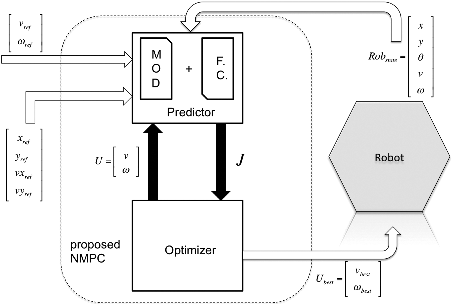
Simulations with both circular-shaped and eight-shaped trajectories were performed comparing the results from three different approaches: an ADC by Martins et al., ³⁸ the classic NMPC, ³⁶ and our proposed NMPC. Figure 4 presents the simulation results from all three control algorithms performing a circular-shaped trajectory. The initial lack of smoothness of our approach observed on the simulation within a circular trajectory is due to the instantaneous effort to converge to the trajectory tracked. This caused an initial bad behavior converging afterwards. This does not concerns the application due to the fact that it can be removed with better gain values found from this or another tuning approach. The tuning approach used here does not guarantee optimality; therefore, it could be found values that would smooth this behavior. This is confirmed by Figure 5(a) that presents the trajectory tracking error comparing the performance of all three controllers over time. Comparing the performance between all three approaches, we have a better result with the proposed NMPC.

Figure 4.

Simulation using the Pioneer 3-DX robot model performing a circular trajectory. (a) ADC ³⁹ , (b) NMPC, and (c) proposed NMPC. ADC: Adaptive dynamic controller.

Figure 5.

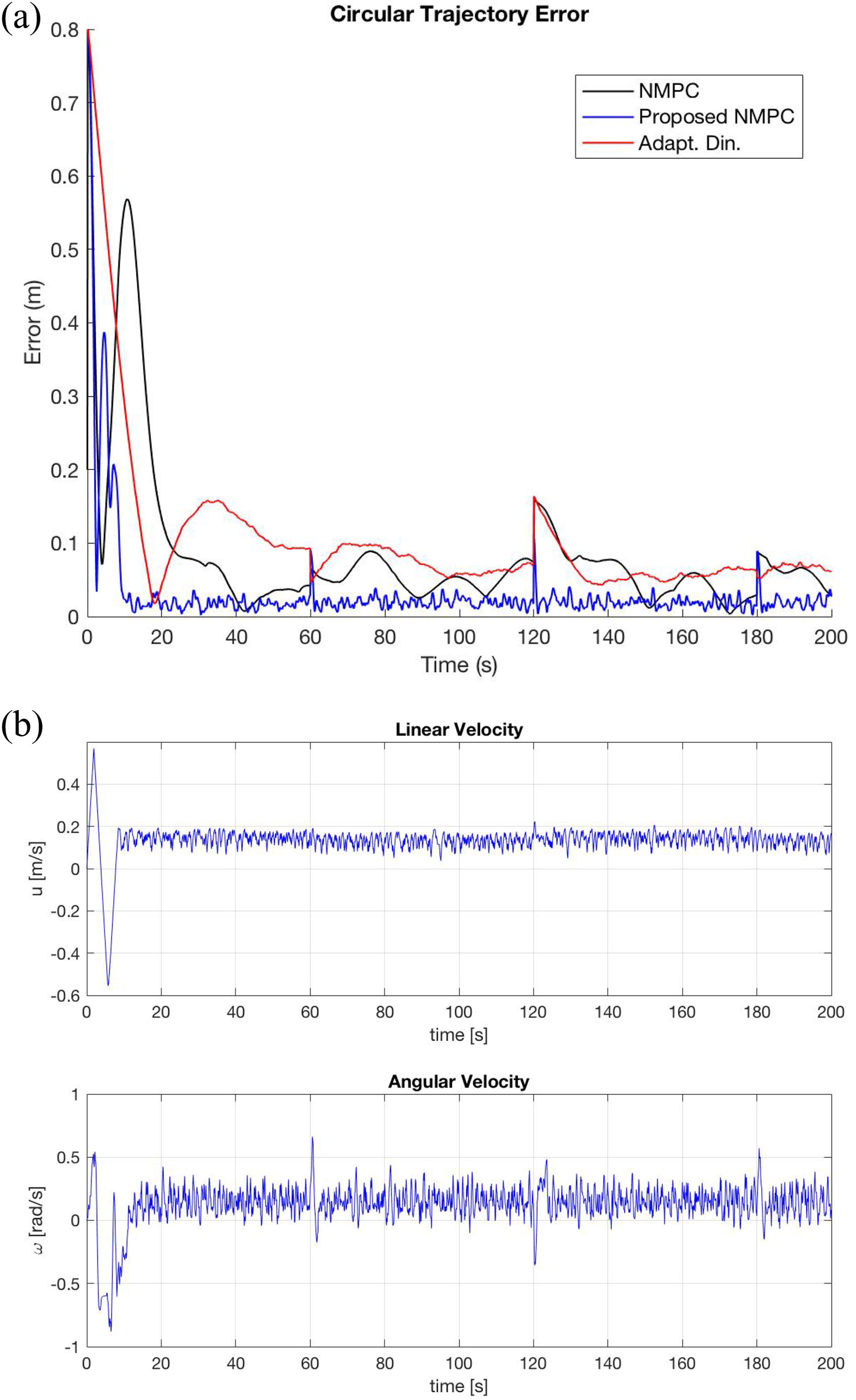
Circular-shaped trajectory error (a) and proposed NMPC output (b) for the Pioneer 3-DX robot model performing a circular-shaped trajectory.

We also present here the output of the proposed NMPC controller’s values over time (Figure 5(b)) for the circular-shaped trajectory. Furthermore, Table 2 presents the comparison of all three controllers through four indexes, ³⁸ namely integral absolute error (IAE), integral square error (ISE), integral of time-weighted squared error (ITSE), and integral time-weighted absolute error (ITAE), which also demonstrate the efficiency of our approach.

Table 2.

Controllers’ performance: Circular-shaped trajectory.

Controller	IAE	ISE	ITSE	ITAE
Adaptive dynamic	20.99	4.65	125.11	1.43e3
NMPC	17.58	3.89	108.78	1.20e3
Proposed NMPC	6.37	1.26	12.08	0.40e3

IAE: integral absolute error; ISE: integral square error; ITSE: integral of time-weighted squared error; ITAE: integral time-weighted absolute error.

Figure 6 presents the simulation results from all three control algorithms performing an eight-shaped trajectory. Simulations of the eight-shaped trajectory also demonstrate the efficiency of our approach over the classic NMPC controller and the ADC by analyzing Figure 7(a) that presents the trajectory tracking error comparing the performance of all three controllers over time. Note that the trajectory obtained using our approach converges rapidly to the steady-state point and tries to maintain the steady-state error at minimum. Note also that there are fluctuations at the position (0.5, 2), (0.75, 0.15), and (0.75, 1.4), which are due to the increase in nonlinearity of the closed loop system in this trajectory. These fluctuations can be higher or lower depending on the controller used. Note that these fluctuations are not present neither in the circular trajectory nor during the following real robot experiments that will be presented. If compared with the fourth simulation of the work by Martins et al., ³⁸ one can note also that the mean error value of the ADC was reduced, reaching a mean value of 0.05 m, while in our proposed NMPC, the mean error value was reduced, reaching a mean value of 0.025 m.

Figure 6.

Simulation using the Pioneer 3-DX robot model performing an eight-shaped trajectory. (a) Adaptive dynamic controller ³⁹ , (b) NMPC, and (c) proposed NMPC.

Figure 7.

Eight-shaped trajectory error (a) and proposed NMPC output (b) for the Pioneer 3-DX robot model performing an eight-shaped trajectory.

The efficiency of our approach can be analyzed through the controller’s output signals (Figure 7(b)) and through Table 3. This table presents the comparison of all three controllers through four indexes used in the eight-shaped trajectory. This table demonstrates the efficiency of our approach by showing that it reached the lower indexes values. In both circular-shaped trajectory and eight-shaped trajectory, our approach reached better results than the other approaches with an average improvement of 2.5 times.

Table 3.

Controllers’ performance: Eight-shaped trajectory.

Controller	IAE	ISE	ITSE	ITAE
Adaptive dynamic	11.23	0.99	47.30	0.82e3
NMPC	28.99	5.34	533.19	2.90e3
Proposed NMPC	5.11	0.21	17.19	0.49e3

IAE: integral absolute error; ISE: integral square error; ITSE: integral of time-weighted squared error; ITAE: integral time-weighted absolute error.

Experiments

Also, we performed two sets of real robot experiments similar to the simulation trajectories. The first trajectory is a circular-shaped trajectory with radius = 1 m while the second trajectory is an eight-shaped trajectory with the radius = 1 m and the total length = 2 m. The same offset in the circular path given by the trajectory generation in simulations can be seen also in the real robot experiments. To determine the robots position, we used a common vision-based tracking system.

The robot starts from the initial pose $X_0{=[0,0,0]}^{\text{T}}$ (m, m, rad) in both set of experiments. Under tracking, the controller update time step for the Turtlebot 2 robot was 0.04 seconds with number of maximum iterations I_max = 15, prediction horizon N_p = 7, and control horizon N_u = 2. At any trajectory, the final controller gain values for the proposed NMPC used in the Turtlebot 2 robot were obtained through the method by Nascimento et al. ⁴⁰ are λ₁ = 800, λ₂ = 400, and λ₃ = 0.05.

Figure 8 presents the results of the circular-shaped trajectory performed by the Turtlebot 2 using the proposed NMPC. We can observe that the robot converges rapidly to the path minimizing the distance error to mean value of 0.03 m. The three spikes we see in the plot (Figure 8(b)) are due to the change in the path radius (offset of −0.1 m as above mentioned). Different from simulations, the output signals are more “messy” due to sensor noise.

Figure 8.

Performance of Trutlebot 2 mobile robot using the proposed NMPC to track the circular-shaped trajectory. The reference and tracked path (a), the distance error between the reference and performance trajectories (b), the control outputs (c), and the XY error over time (d) are presented here.

Figure 9 also presents the Turtlebot 2 performance results but for the eight-shaped trajectory. The robot also converges rapidly to the path minimizing the distance error to mean value of 0.03 m. The single spikes we see in the plot (Figure 9(b)) at 150 s are due to slip, a problem that we will focus in future works. Both Figures 8(c) and 9(c) also present the velocity saturation imposed on the Turtlebot robot as a velocity constraint. These constraints are common on real robot experiments for safety issues and where considered during the optimization loop. In simulation, however, despite it being unnecessary, we used the velocity saturation but limited it to the robot maximum speed. Nevertheless, the robot never reached those saturation speeds.

Figure 9.

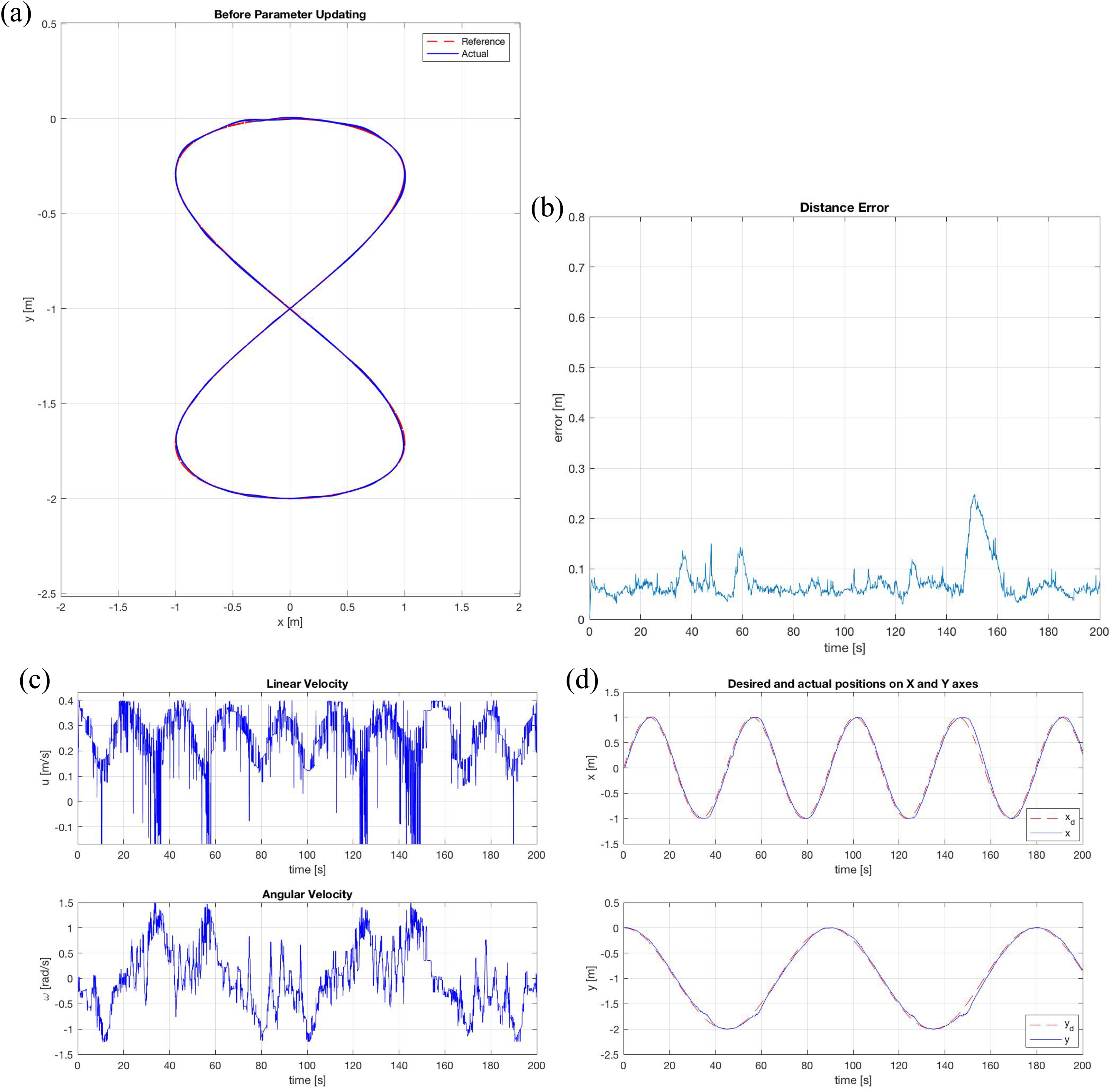
Performance of Trutlebot 2 mobile robot using the proposed NMPC to track the eight-shaped trajectory. The reference and tracked path (a), the distance error between the reference and performance trajectories (b), the control outputs (c), and the XY error over time (d) are presented here.

Finally, Table 4 presents the control indexes (IAE, ISE, ITSE, and ITAE) for both circular-shaped and eight-shaped trajectory experiments with Turtlebot 2 and the proposed NMPC. As in simulations, the values for the eight-shaped trajectory were lower than the circular-shaped trajectory due to the change in radius that occurred three times in the circular-shaped trajectory experiment.

Table 4.

Proposed NMPC performance in real robot experiments.

Trajectory	IAE	ISE	ITSE	ITAE
Circular-shaped	17.12	4.62	116.07	1.26e3
Eight-shaped	14.57	1.30	146.48	1.52e3

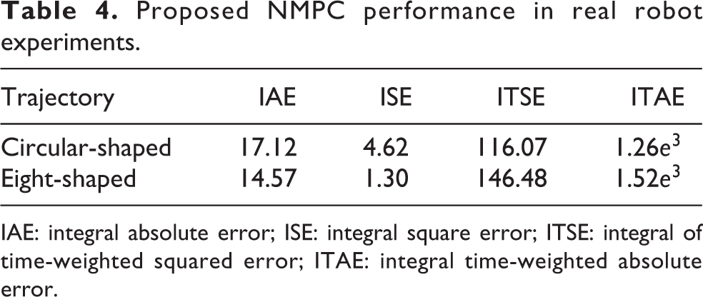
IAE: integral absolute error; ISE: integral square error; ITSE: integral of time-weighted squared error; ITAE: integral time-weighted absolute error.

Conclusion

This article proposes a set of modifications on the classic NMPC controller applied to trajectory tracking control of nonholonomic systems. We have demonstrated that the use of the classic tracking error approach in a nonlinear model predictive controller is not as effective as observing the trajectory coordinates and desired velocities as the position and velocity of a virtual leader to be followed. The change in the prediction model, cost function, and minimization algorithm increased by almost three times the whole algorithm efficiency.

The proposed approach increases the closed loop nonlinearities enabling the mobile robot to perform both trajectories without the need to retuning. The cost function is also adaptable to receive new penalization terms such as to maximize obstacle avoidance and minimize the error in perception of a target. Both modifications are the starting subject of our future works.