Sage Journals: Discover world-class research

Abstract

Nonlinear dose–response relationships exist extensively in the cellular, biochemical, and physiologic processes that are affected by varying levels of biological, chemical, or radiation stress. Modeling such responses is a crucial component of toxicity testing and chemical screening. Traditional model fitting methods such as nonlinear least squares (NLS) are very sensitive to initial parameter values and often had convergence failure. The use of evolutionary algorithms (EAs) has been proposed to address many of the limitations of traditional approaches, but previous methods have been limited in the types of models they can fit. Therefore, we propose the use of an EA for dose–response modeling for a range of potential response model functional forms. This new method can not only fit the most commonly used nonlinear dose–response models (eg, exponential models and 3-, 4-, and 5-parameter logistic models) but also select the best model if no model assumption is made, which is especially useful in the case of high-throughput curve fitting. Compared with NLS, the new method provides stable and robust solutions without sensitivity to initial values.

Keywords

evolutionary algorithm hillslope model parameter estimation nonlinear regression model selection

Introduction

The dose–response relationship is a cornerstone of toxicology and pharmacology. It is commonly observed in many cellular, biochemical, and physiologic processes in the presence of varying levels of biological, chemical, or radiation stress. Toxicologists and pharmacologists routinely conduct dose–response experiments to explore the effects of compounds or substrates at various concentrations on biological systems, such as cells, tissues, and whole organisms. Data generated from experiments are subsequently utilized to model dose–response relationships and fit curves, which allows scientists to interpolate or extrapolate missing information.¹

Dose–response modeling has been extensively studied in the past few decades, as it is of key importance in toxicology and pharmacology. The dose–response relationship usually resembles a sigmoidal curve with both upper and lower limits. Both parametric and nonparametric models have been proposed to fit sigmoidal curves. Considering that nonparametric models are not very reliable with a small sample size, which is often the case in experimental designs of dose–response studies, parametric models are preferred for dose–response curve fitting. The most commonly used approach to fit nonlinear parametric models is NLS.² In general, NLS estimates model parameters by making linear approximations and then refines the parameters by successive iterations based on the sum of squares. There are many algorithms available for NLS implementation, such as the Gauss-Newton algorithm,³ the Levenberg-Marquardt algorithm,⁴ and the NL2SOL algorithm.⁵ Although NLS is a very powerful method for modeling nonlinear relationships, it has several drawbacks. First, it is highly sensitive to the choice of starting values.² The initial parameter values of NLS must be close to the true values, otherwise there may be no convergence. Moreover, poor initial values may lead to the algorithm settling into local minimum solutions instead of globally optimal solutions that define the least squares estimates.²

The increasing use of high-throughput screening (HTS) magnifies the limitations of NLS in dose–response modeling. High-throughput screening is widely used in the pharmaceutical and biotechnology fields, and in academic, and federal institutes.^6
-8 Specifically, it is being applied in the discovery of toxicity,⁹ biopharmaceuticals,¹⁰ cosmetics, catalysts,¹¹ pesticide research,¹² and plant science.¹³ Such screens assay hundreds of thousands of chemical compounds or organic molecules simultaneously against specific targets under given conditions. Dose–response modeling for HTS data is challenging, not only because of the large size and the limitations of NLS but also because the data for each curve are sparse. For example, there are typically only 6 to 10 concentrations for each sample across many of even the most high-profile and high-impact experiments.^14,15 Additionally, many of these experiments also screen a number of individual cell lines. It is reasonable to expect that the response pattern of each response curve will be different across chemicals in a screen, as well as across individuals within a screen for just one chemical. Restricting the type of models that can be fit greatly limits the impact of such experiments.⁶ Additionally, considering that thousands of curves must be estimated, it is impractical to fit each one manually. Therefore, it is necessary to develop computational tools that can automatically model high-throughput dose–response data with minimal human supervision.

A number of software and R packages are currently available for curve fitting, such as benchmark dose software (BMDS),¹⁶ nlstools, MCPMod, drc, and DoseFinding. However, few of these successfully address both concerns mentioned above: the sensitivity of initial values in NLS and high-throughput curve fitting. Almost all require manual intervention during the curve fitting process. For example, US Environmental Protection Agency developed a BMDS to help Agency risk assessors facilitate applying benchmark dose methods.¹⁶ Although it is highly impactful and widely used, this software still requires extensive human interaction when dealing with high-throughput dose–response data. To address concerns about initial value sensitivity in NLS, Beam and Motsinger-Reif¹⁷ implemented an evolutionary algorithm (EA) for dose–response modeling (EADRM) and achieved good results. Evolutionary algorithms are adaptive heuristic search approaches and global optimization techniques widely used in artificial intelligence and computing.¹⁸ Originally motivated by Charles Darwin’s theory of natural evolution and survival of the fittest, EAs are capable of solving complex optimization issues by imitating evolutionary concepts such as reproduction, mutation, recombination, and selection.¹⁸ Unlike traditional optimization techniques that attempt to determine a single, best solution, EAs generate a population of random possible solutions. Each solution is evaluated by a fitness function, and mutations are then induced to more fitted solutions to create the next-generation population. The selection process continues until the optimal solution is found.¹⁹

In the present study, to further address challenges in high-throughput curve fitting, we expand the functionalities of EADRM by adding a broad range of dose–response models such as exponential models and 3-, 4-, and 5-parameter logistic models. We also compare different model selection criteria (ie, Akaike information criterion [AIC], Bayesian information criterion [BIC], and R ²) to achieve the best model selection performance. Additionally, we use extensive simulations and real-data analysis to demonstrate our new approach. We show that the EA approach can not only fit the most commonly used nonlinear dose–response models but also select the best model if no model assumption is made, which is especially useful for high-throughput curve fitting. Compared with NLS, this approach provides stable and robust solutions without sensitivity to initial values.

Materials and Methods

Evolutionary Algorithm

Evolutionary algorithms as a class are heuristic-based approaches to solve problems that cannot be easily solved in polynomial time and/or in tandem with other methods, acting as a quick way to find a somewhat optimal starting place for another algorithm to work off of.²⁰ The premise of any EA is to mimic the process of natural selection to evolve models that fit a given application—in this case, finding a dose–response curve model. An EA contains 4 overall steps: initialization, selection, genetic operators, and termination. These steps each correspond, roughly, to a particular facet of natural selection and provide easy ways to modularize implementations of this algorithm category. Simply put, in an EA, fitter members will survive and proliferate, while unfit members will die off and not contribute to the gene pool of further generations, much like in natural selection. In this study, we use a very general EA approach as described in detail below.

Additionally, we compared the curve fitting performance of our EA approach with another popular EA, differential evolution (DE).²¹ Differential evolution is a relatively new EA and is a powerful stochastic real-parameter optimization algorithm in current use.²² Differential evolution operates through similar computational steps as employed by a standard EA and is population-based like genetic algorithms. However, unlike traditional EAs, the DE variants perturb the current-generation population members with the scaled differences of randomly selected and distinct population members. Specifically, the candidate solutions are initialized randomly at first. Then at each iteration and for each candidate solution x, perform the following steps:

Generate a trial vector: v = a + (b − c) / 2, where a, b, and c are 3 distinct candidate solutions picked randomly among the population.

Randomly swap vector components between x and v to produce v′. At least one component from v must be swapped.

Replace x in the population with v′ only if it is a better candidate.^22,23

Built-In Dose–Response Models

Log-logistic models, including 3-, 4-, and 5-parameter logistic models, are by far the most commonly used dose–response models. Therefore, their corresponding model functions are built into our tool. In addition, an exponential model is also incorporated into our tool because the dose–response relationship may sometimes not resemble a sigmoid curve.

Equations 1 to 3 show 3 log-logistic models:

Three - parameter model: f (x) = \frac{d}{(1 + exp (b \times (log (x) - log (e))))},

Four - parameter model: f (x) = c + \frac{d - c}{(1 + exp (b \times (log (x) - log (e))))},

Five - parameter model: f (x) = c + \frac{d - c}{{(1 + exp (b \times (log (x) - log (e))))}^{f}} .

In these log-logistic models, x is a dose value and (x) denotes a corresponding response value. b, which is often called the hillslope, is a coefficient denoting the steepness of the dose–response curve. c and d are called E _min and E _max, respectively, and represent the lower and upper asymptotes or limits of the response. e represents EC₅₀, which is the concentration of a drug that gives a half-maximal response. f is an asymmetry factor. f = 1 suggests a symmetrical curve around the inflection point, which is a 4-parameter model.

Equation 4 shows an exponential model:

f (x) = β \times exp (λ x),

where β is a scale factor and λ is a growth factor.

Users can choose any model to fit their data. If users do not know which model to use, the tool automatically selects the best model.

Implementation of EA

An EA was implemented to optimize parameters in the selected model. The following describes the optimization process.

A. Initialization

For a faster convergence rate, the initial solution is generated using sensible initialization. That is, the initial parameter values are created based on previous curve fitting experience. For log-logistic models, E _min and E _max are set to the minimum and maximum response values, respectively. EC₅₀ is set to the average of the minimum and maximum concentration values. The hillslope is set to 2.5, and the asymmetry factor is set to 1. For exponential models, the scale factor is set to 1, and the growth factor is set to 2.5. Subsequently, the initial solution is mutated up to ±100% to generate a population with a user-defined number of random possible solutions. Further, the hillslope value and the scale factor are provided with a negative sign with a 50% chance. If users choose a specific model to fit their data, all solutions will use that model. If no model is specified, 25% of the solutions will use each of the 4 models mentioned above.

B. Evaluation

Each of the random solutions is evaluated by a fitness function to determine how well it fits the data. The fitness function in this study is the BIC, as shown below:

BIC = p \times ln (n) - 2 \times ln (L)

where p represents the number of parameters, n is the sample size, and L is the maximum likelihood of the model. The lower BIC value signals a better solution. In addition to a fitness function, the BIC also serves as a criterion for model selection, as it gives a penalty on the number of parameters.

C. Selection

Tournament selection is used to select the best solutions from a population.²⁴ Specifically, the user-defined number of solutions (tournament size N) is randomly selected from the population and then the fitness function is used to select the solution with the best fitness from the N solutions. The process is repeated T times (number of tournaments), the value of which is specified by the user.

D. Mutation

The solutions selected from the current generation are mutated up to ±10% to create the next-generation population of size P, which is specified by the user.

E. Termination

The selection and mutation processes are repeated until the user-defined number of generations is reached. Finally, the best solution is selected.

Simulation Data Set and High-Throughput Experimental Data Set

To evaluate the performance of our new tool, real data were used to generate semisynthetic simulations and to demonstrate the performance of the methods on real data. Brown et al²⁵ performed a high-throughput experiment evaluating the association of genetic variants with differential dose response with anticancer drugs. Lymphoblastoid cell lines (LCLs) were used to perform genome-wide association mapping of the cytotoxic response of 520 European Americans to 29 different anticancer drugs. Details of the experiment and previous results can be found in several previous publications.^25,26 The LCL model has been successfully used to evaluate dose response in a broad range of applications in pharmacology and toxicology.²⁷

Briefly, Epstein-Barr virus immortalized LCLs were seeded in 384-well plates containing temozolomide (0.10, 0.25, 0.50, 1.0, 2.0, 2.5 mM) obtained from LKT Laboratories.²⁵ After incubation, the results were quantified on an Infinite F200 microplate reader.²⁵

A 7-stage quality control (QC) pipeline was used for the cytotoxicity data detailed in a previous study,²⁸ including the removal of plates containing mostly dead cells, imputation of grossly errant raw fluorescence units (RFUs), QC for the negative control RFUs, and QC for drug vehicle RFUs. The following equation was utilized to compute the percent viability²⁵:

Y_{i j k l} = \frac{Y_{i j k l, r a w} - V_{i j, 10 % DMSO}}{V_{i j, 0.2 % DMSO} - V_{i j, 10 % DMSO}},

where Y_ijkl , Raw is the RFU of the jth cell line from the ith genotype, exposed to the kth drug concentration for the lth quadruplicate replication, and Y_ijkl is the corresponding estimated percent viability. V_ij _,10%DMSO and V_ij _,0.2%DMSO are the average RFUs for the negative control and vehicle wells, respectively.²⁵

The final QC procedure includes the following steps. First, ensure that every dose–response curve is monotonic.²⁵ Second, scale the data so that the mean viability at the lowest drug concentration is 1.0.²⁵ Third, remove assays containing viabilities above 1.3 or below −0.05.²⁵ These QC steps result in cleaning 0.5% to 1.5% of data.²⁵

The data for response to temozolomide from this experiment were used to create simulated data. To generate simulated data sets, small amounts of variation were added to the response values. The variation follows a truncated normal distribution with mean 0 and a standard deviation (SD) of 1, bounded between −1.5 and 1.5.

The real data were also used to demonstrate the methods performance in context of experimental results. Previous results had shown a strong association with differential response to temozolomide with a single-nucleotide polymorphism (SNP) in the O(6)-methylguanine-DNA methyltransferase (MGMT) gene.²⁵ The SNP significantly changes gene expression, in return changes the response to the drug. This gene has been shown to be associated with patient survival in clinical data.^29,30

Tool Performance Evaluation

Understanding the impact of parameter choices is important in any EA.^31,32 The simulated data sets were used to investigate the influence of EA parameters on the convergence rate. Evolutionary algorithm parameters include initial population size, equilibrium population size, and initial tournament size. For each parameter being tested, a series of values were evaluated, while other parameters were fixed to the following values: initial population—5000, equilibrium population—200, and tournament size—25. The generated raw data were subsequently averaged.

To tune EA parameters for better performance, 6 different combinations of parameters were evaluated to determine which has the best performance in terms of fitness, variation, and execution time. The simulation experiments were repeated 20 times for each set of parameters, and the mean fitness values, SD, and mean computation time were then calculated.

To compare the initial value sensitivity between EA and NLS, we set up 7 widely ranging starting values for EC₅₀, from 0.0001 to 1000, and then recorded the corresponding results for nonlinear fit with EA and 2 NLS methods: NL2SOL³³ and Gauss-Newton.³⁴

To investigate this tool’s performance on model selection, 1000 simulation data sets were generated based on a 3-parameter model with added noise magnitude SD 0.01 and another 1000 with added noise magnitude SD 0.1. The tool was then employed to select the appropriate model using different fitness functions (AIC, BIC, and R ²), and the percentage of selecting the “true” 3-parameter model was calculated.

To demonstrate the utility of using the evolutionary approach, we compared our model fits to curves generated in a random search. To compare this new tool’s performance on high-throughput curve fitting against current computational tools, namely, R package drc and R package DEoptim, our tool was used to fit a high-throughput experimental data set. The mean and SD of R ² values for all curve fitting were recorded. Additionally, the corresponding bias and fitness were also summarized. Moreover, t test as well as analysis of variance (ANOVA) with post hoc Tukey Honest Significant Difference (HSD) tests were performed to check if the curve fitting performance of our method was significantly better than other methods.

All the code and simulations were written and conducted using the R language. All simulations were conducted in Ubuntu 16.04 LTS using an Intel Xeon Processor E5-2620. An R package implementation is available through CRAN (EADRM.R).

Results

Influence of EA Parameters on Convergence Rate

As evolutionary computation is an iterative optimization procedure, it is of great importance to explore the speed at which an EA converges. Previous studies suggest that the performance of EA is heavily influenced by several parameters such as initial population size, equilibrium population size, and initial tournament size. Therefore, it is necessary to investigate the effect of these parameters on the convergence rate.

Simulation was performed using data generated from 5-parameter logistic models. For each parameter examined, a series of values were evaluated while other parameters were fixed to the following values: initial population—5000, equilibrium population—200, and tournament size—25. The numerical experiments to estimate both convergence rate and running time were performed 50 times, and the raw data were subsequently averaged. As illustrated in Figure 1, all 3 parameters demonstrate similar patterns regarding convergence rate. In general, a small parameter size results in premature convergence on areas of poor fitness, while a relatively large parameter size usually has a good convergence rate. However, the further increase in an already large parameter size does not lead to faster convergence. Figure 2 shows the relationship between a single parameter’s size and execution time. It suggests that there is an exponential trade-off between execution time and tournament size. Additionally, there is a linear trade-off between execution time and initial population size as well as equilibrium population size.

Figure 1.

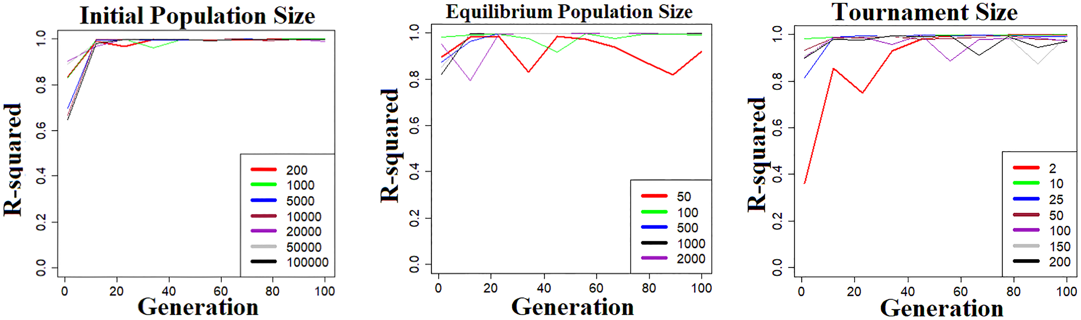
Effect of evolutionary algorithm parameter size on convergence rate. The x-axis represents the number of generations and the y-axis is the R ² value.

Figure 2.

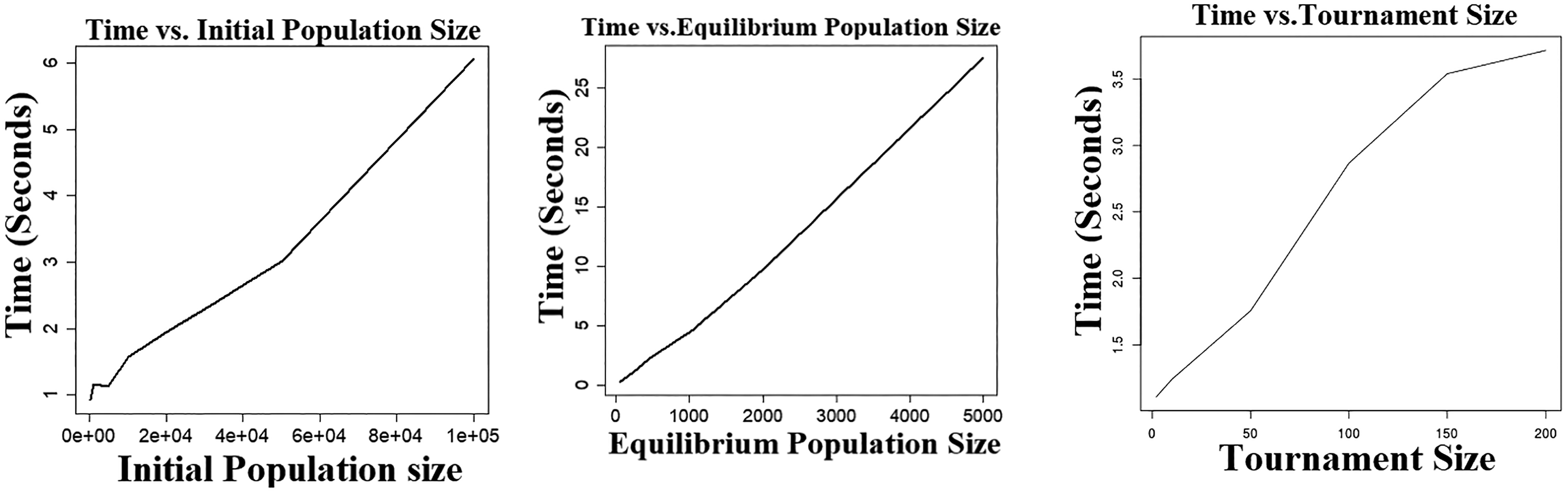
Execution time versus evolutionary algorithm parameter size. The x-axis represents parameter size and the y-axis represents corresponding execution time (seconds).

Parameter Selection in EA

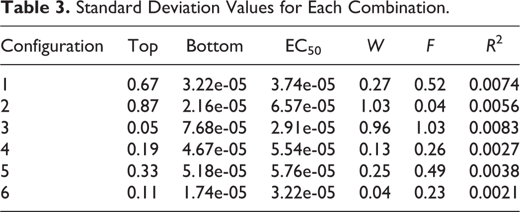
Since EA parameters have a significant impact on the efficiency and ability of EA optimization, it is important to tune these parameters to achieve good performance. In this simulation, 6 parameter combinations (Table 1) were evaluated to determine which has the best performance in terms of fitness, variation, and execution time. The simulation experiments were repeated 20 times for each set of parameters, and the mean fitness values, SD, and mean computation time were then calculated. The results are given in Tables 2 to 4.

Table 1.

Configuration Parameter Values for Each Combination.

Configuration	1	2	3	4	5	6
Initial population	5000	20 000	5000	5000	20 000	10 000
Equilibrium population	200	200	1000	200	5000	1000
Tournament size	25	25	25	100	500	300

Table 2.

Average Parameter Values for Each Combination.

Configuration	Top	Bottom	EC₅₀	W	F	R ²
1	0.73422545	0.05123052	0.01137427	2.37301427	0.86565270	0.99913
2	0.64101163	0.00621338	0.00557989	3.50794703	0.31203447	0.99951
3	0.77019582	0.05667068	0.01129192	2.14239609	1.09939554	0.99975
4	0.718118531	0.068346785	0.007967174	2.757923304	0.545626302	0.99983
5	0.666575395	0.072511186	0.005997677	2.752326288	0.656949838	0.99996
6	0.795849688	0.094701674	0.006332252	2.645839398	0.456528064	0.99992

Table 3.

Standard Deviation Values for Each Combination.

Configuration	Top	Bottom	EC₅₀	W	F	R ²
1	0.67	3.22e-05	3.74e-05	0.27	0.52	0.0074
2	0.87	2.16e-05	6.57e-05	1.03	0.04	0.0056
3	0.05	7.68e-05	2.91e-05	0.96	1.03	0.0083
4	0.19	4.67e-05	5.54e-05	0.13	0.26	0.0027
5	0.33	5.18e-05	5.76e-05	0.25	0.49	0.0038
6	0.11	1.74e-05	3.22e-05	0.04	0.23	0.0021

Table 4.

Execution Time for Each Configuration.^a

Configuration	1	2	3	4	5	6
Time (seconds)	23.832	58.327	482.901	141.635	2612.074	1025.689

^a Simulations were conducted in Ubuntu 16.04 LTS using an Intel Xeon Processor E5-2620.

As summarized in Table 2, all 6 sets of parameters returned very good solutions. Set 5 had the best fitness, followed by set 6 and set 3. Table 3 suggests that set 6 generated the most consistent results, followed by set 4 and set 5. In addition, set 1 had the fastest execution time of 23.832 seconds, followed by 58.327 seconds for set 2, presented in Table 4. Although set 5 had slightly better fitness than set 6, it ran about 2.5 times slower than set 5. Considering these factors, set 6 had the best overall performance and was thus selected for the default parameter settings.

Comparison With Random Search

The random search was run so that an equal number of random curve fits to the number of curves evaluated within the EA across all generations. Table 5 presents the results for the best fits generated by the 2 approaches. The EA algorithm very clearly outperforms the random search.

Table 5.

Fitness Summary of EA and Random Search on High-Throughput Simulation Data.

	EA	Random search	P value of t test comparing EA and the random search
Mean of R ²	0.9893765	0.3795297	4.86E-08
SD of R ²	0.0076938	0.5957368	8.73E-14

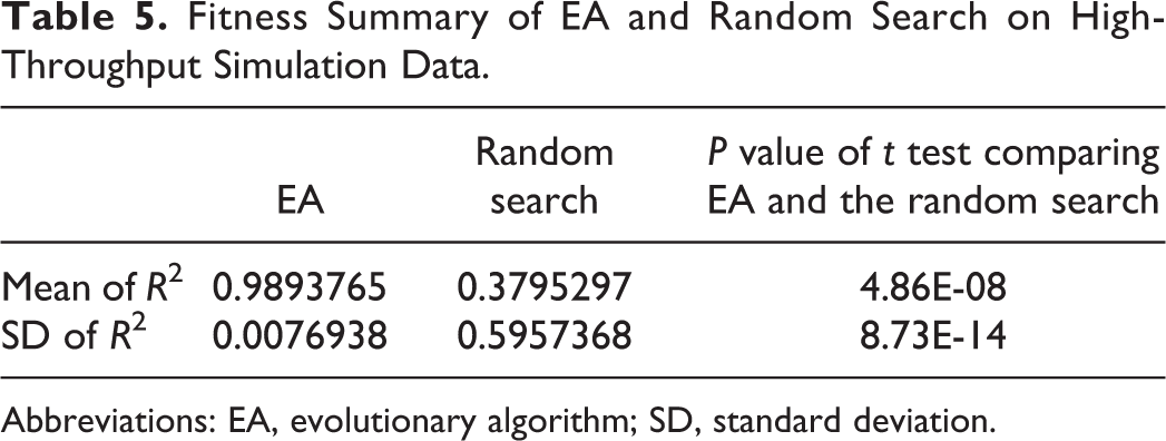
Abbreviations: EA, evolutionary algorithm; SD, standard deviation.

Comparison of Initial Value Sensitivity Between EA and NLS

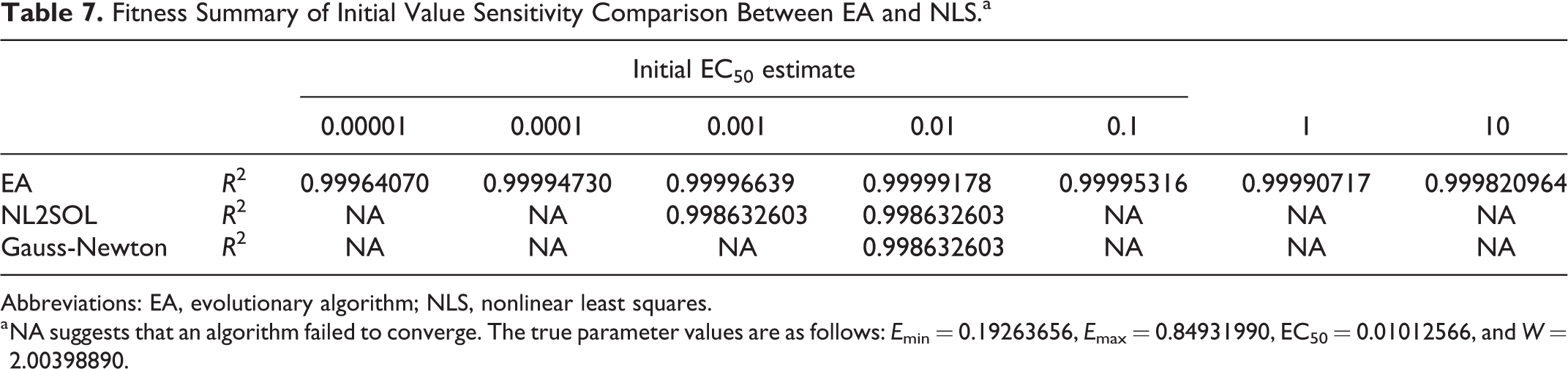
Nonlinear least squares is a powerful method for modeling nonlinear relationships but has a major disadvantage: sensitivity to the starting values. The initial parameter values of NLS must be close to the true values, otherwise it may not converge or may converge to a local minimum. In this study, the EA is evaluated to assess whether it can overcome this disadvantage of NLS. Considering that EC₅₀ is the most sensitive parameter in the nonlinear-response model, we set up 7 widely ranging starting values for EC₅₀, from 0.00001 to 10 and then recorded the corresponding results for nonlinear fit with EA and 2 NLS methods: NL2SOL and Gauss-Newton. The simulation was conducted using the curve parameters from a 4-parameter logistic model. Tables 6 and 7 summarize the results.

Table 6.

Bias Summary of Initial Value Sensitivity Comparison Between EA and NLS.^a

	Initial EC₅₀ estimate
EA	0.00001	0.0001	0.001	0.01	0.1	1	10
E _min	0.01575936	−0.00053479	0.00070563	0.00107233	0.00347825	0.00208942	0.012794713
E _max	0.00581124	0.00319672	−0.00153412	0.00083525	−0.00153153	0.00486367	−0.002855443
EC₅₀	−0.00040074	−0.00009231	0.00016316	0.00016299	0.00022918	7.664E-05	1.1363E-05
W	−0.11399323	0.02740953	0.02197609	−0.00803709	0.01748289	0.00881108	0.118607461
NL2SOL
E _min	NA	NA	0.001067345	0.000980467	NA	NA	NA
E _max	NA	NA	0.001200976	−0.001009779	NA	NA	NA
EC₅₀	NA	NA	−0.00986743	0.009867433	NA	NA	NA
W	NA	NA	0.039838297	0.039838195	NA	NA	NA
Gauss-Newton
E _min	NA	NA	NA	0.001279372	NA	NA	NA
E _max	NA	NA	NA	−0.000900964	NA	NA	NA
EC₅₀	NA	NA	NA	0.000286743	NA	NA	NA
W	NA	NA	NA	−0.04198383	NA	NA	NA

Abbreviations: EA, evolutionary algorithm; NLS, nonlinear least squares.

^a NA suggests that an algorithm failed to converge. The true parameter values are as follows: E _min = 0.19263656, E _max = 0.84931990, EC₅₀ = 0.01012566, and W = 2.00398890.

Table 7.

Fitness Summary of Initial Value Sensitivity Comparison Between EA and NLS.^a

		Initial EC₅₀ estimate
		0.00001	0.0001	0.001	0.01	0.1	1	10
EA	R ²	0.99964070	0.99994730	0.99996639	0.99999178	0.99995316	0.99990717	0.999820964
NL2SOL	R ²	NA	NA	0.998632603	0.998632603	NA	NA	NA
Gauss-Newton	R ²	NA	NA	NA	0.998632603	NA	NA	NA

Abbreviations: EA, evolutionary algorithm; NLS, nonlinear least squares.

^a NA suggests that an algorithm failed to converge. The true parameter values are as follows: E _min = 0.19263656, E _max = 0.84931990, EC₅₀ = 0.01012566, and W = 2.00398890.

As expected, both NLS methods produced good solutions with optimum model parameters when the initial EC₅₀ value is close to the true value of 0.01, whereas inappropriate starting values of EC₅₀ led to convergence failure or poor fitness, as presented in Tables 6 and 7. Compared with NLS, EA produced efficient and robust solutions with better fitness for the full range of initial EC₅₀ values, suggesting that EA is relatively insensitive to the choice of initial parameter values.

Model Selection Performance

In addition to modeling nonlinear relationships, our tool can also select the best model from the most commonly used nonlinear dose–response models, including exponential models and 3-, 4-, and 5-parameter logistic models. A major part of the innovation of this method is that it allows analysts to be agnostic to the optimal functional form for the curve fit. To investigate this tool’s performance on model selection, 1000 simulation data sets were generated based on a 3-parameter model with added noise magnitude SD 0.01 and another 1000 with added noise magnitude SD 0.1. The tool was then employed to select the appropriate model using different fitness functions (AIC, BIC, and R ²). These 3 popularly used fitness functions were compared in regard to their performance to consistently select the correct functional form as the best final model. The percentage of selecting the “true” 3-parameter model was calculated and Table 8 summarizes the results. The results indicate that BIC had the best performance among the 3 fitness functions. It selected the true 3-parameter model in 65% of the data sets with noise SD 0.01 and in 52% of the data sets with noise SD 0.1.

Table 8.

Model Selection Frequency for the Different Measures of Goodness of Fit.^a

	Model	AIC	BIC	R ²
SD = 0.01	5-Parameter model	0	4	8
	4-Parameter model	0	31	67
	3-Parameter model	3	65	25
	2-Parameter model	97	0	0
3-Parameter model %		3%	65%	25%
SD = 0.1	5-Parameter model	0	10	5
	4-Parameter model	0	38	52
	3-Parameter model	1	52	43
	2-Parameter model	99	0	0
3-Parameter model %		1%	52%	43%

Abbreviations: AIC, Akaike information criterion; BIC, Bayesian information criterion; SD, standard deviation.

^a Three-parameter model is the “true” model.

Comparison With Current Computational Tools on High-Throughput Data Analysis

A significant amount of dose–response data is being generated thanks to advances in HTS technology. To evaluate our tool’s performance on high-throughput data analysis, dose–response curve fitting was performed on simulated data sets and our tool was compared with a popular R package DEoptim, which implements the DE algorithm for global optimization. In this comparison, EA automatically selected dose–response models, while Deoptim used 3-, 4-, and 5-parameter dose–response models separately. Table 9 displays the results. It shows that EA has better fitness and higher stability than Deoptim. Furthermore, we performed ANOVA with post hoc test on mean of R ² and SD of R ² for EA versus DEoptim. For mean of R ², the P values of EA versus DEoptim 3-parameter and EA versus DEoptim 4-parameter were .023245 and .046371, respectively. For SD of R ^2HueD_Ref2, the P values of EA versus DEoptim 3-parameter, EA versus DEoptim 4-parameter, and EA versus DEoptim 5-parameter were .000029, .000348, and .000395, respectively. These P values suggest that the high-throughput curve fitting performance of EA is significantly better than DEoptim in terms of fitness and stability.

Table 9.

Fitness Summary of EA and DEoptim on High-Throughput Simulation Data.

	EA	DEoptim -3P	DEoptim -4P	DEoptim -5P
Mean of R ²	0.9899628	0.9757765	0.9815101	0.9880943
SD of R ²	0.008992174	0.01429076	0.004906434	0.004086065

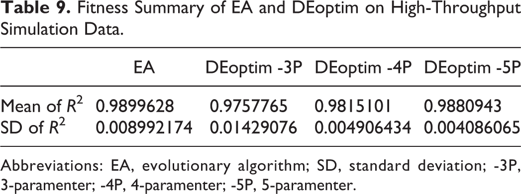
Abbreviations: EA, evolutionary algorithm; SD, standard deviation; -3P, 3-paramenter; -4P, 4-paramenter; -5P, 5-paramenter.

Bias and Variance of Parameter Estimates

Tables 10 displays the results of the bias and evaluations of our method through the simulations, where minimizing both of these measures indicates improved performance. Our results show extremely minimal bias, indicating that the method produces models with both high fitness values and highly accurate parameter estimates.

Table 10.

Bias Summary of EA, DEoptim, and NLS on High-Throughput Simulation Data.

	E _min	E _max	EC₅₀	W
EA	−0.00070563	0.000153412	−0.00016317	0.002197609
DEoptim -3P	0.015759363	−0.00158113	0.000400745	0.113993234
DEoptim -4P	0.012794713	0.002855443	−0.00030185	−0.11860746
DEoptim -5P	0.001259372	−0.00100964	0.000286743	0.091983837
NLS -3P	0.012450104	0.000459162	−0.0003162	0.009005562
NLS -4P	0.010108173	−0.00022554	0.000238942	−0.00936991
NLS -5P	0.001011274	0.000711825	−0.00022617	0.007266751

Abbreviations: EA, evolutionary algorithm; NLS, nonlinear least squares; -3P, 3-paramenter; -4P, 4-paramenter; -5P, 5-paramenter.

The bias of the results from DEoptim and NLS was also calculated and compared to our method (given in Table 10). Generally across parameters, our EA approach demonstrated less bias, and the results of ANOVA with post hoc test comparing them demonstrate it is a significant difference (Table 11).

Table 11.

P Values of ANOVA Post Hoc Tukey HSD for Bias Comparisons Between Different Curve Fitting Methods.

	E _min	E _max	EC₅₀	W
EA vs DEoptim -3P	<0.001	<0.001	<0.001	<0.001
EA vs DEoptim -4P	<0.001	<0.001	<0.001	<0.001
EA vs DEoptim -5P	<0.001	<0.001	<0.001	<0.001
EA vs NLS -3P	<0.001	0.004862	<0.001	0.004028
EA vs NLS -4P	<0.001	0.009378	<0.001	0.003971
EA vs NLS -5P	<0.001	0.002163	<0.001	0.003185

Abbreviations: ANOVA, analysis of variance; EA, evolutionary algorithm; NLS, nonlinear least squares; -3P, 3-paramenter; -4P, 4-paramenter; -5P, 5-paramenter.

Performance on Experimental Data

The real data used were from cytotoxicity assays, where Epstein-Barr virus immortalized LCLs were seeded in plates containing temozolomide. A previous in vitro genome-wide association analysis was conducted with over 2 million QC SNPs and 516 LCLs derived from a Caucasian cohort. It suggests that SNP rs531572 within the MGMT gene is associated with differential response to temozolomide, a DNA alkylator agent used for treatment of adult patients with newly diagnosed glioblastoma multiforme.

In this study, the EA tool was used to verify if these SNPs were potentially functionally relevant. We examined how the genotype was related to differential dose response in terms of EC₅₀ values. Specifically, the EA tool was used to fit dose–response curves from 516 LCLs and estimate corresponding EC₅₀ values. Subsequently, 1-way ANOVA was employed to test for statistical significance. As shown in Figure 3, rs531572 was found to be highly significantly associated with EC₅₀ values. The P value from 1-way ANOVA was .024.

Figure 3.

Box plots for the estimated IC₅₀ for temozolomide by genotype for rs531572.

Additionally, the curve fitting performance of our tool was compared with that of R package DEoptim and R package drc on this experimental data set. In this comparison, EA automatically selected dose–response models, while DEoptim and drc used 3-, 4-, and 5-parameter dose–response models separately. Table 12 summarizes the results. It suggests that EA has better curve fitting performance than DEoptim in terms of fitness and stability. It also shows that EA outperforms drc with 3- and 4-parameter models.

Table 12.

Curve Fitting Performance of EA, DEoptim, and drc on High-Throughput Experimental Data.

	Mean of R ²	SD of R ²
EA	0.950719	0.133827
DEoptim -3P	0.938364	0.317398
DEoptim -4P	0.944635	0.258635
DEoptim -5P	0.949041	0.176714
drc -3P	0.940046	0.181264
drc -4P	0.950469	0.135672
drc -5P	0.955128	0.131873

Abbreviations: EA, evolutionary algorithm; SD, standard deviation; -3P, 3-paramenter; -4P, 4-paramenter; -5P, 5-paramenter.

Software Platform and Availability

This tool was developed using the R statistical language. The code used in this article is available via https://github.com/junmacode/Dose-Response-Modeling-EA. Additionally, an R package EADRM.R is available through CRAN.

Discussion

In the present study, we implemented an EA to model nonlinear dose–response relationships. Our original motivation for this new tool was to address 3 major limitations from current curve fitting tools: the sensitivity of curve fits to initial values with NLS models, the limitation of an analyst having to arbitrarily choose the functional form of a model, and challenges with high-throughput curve fitting due to differences in functional form and other factors across different cell lines, chemicals, and so on.

Our results show that this approach provides stable and robust solutions without sensitivity to initial values. As shown in section “Results,” in spite of dramatically different starting values (from 0.0001 to 1000), EA produced excellent solutions and converged to almost the same parameter values. Unlike NLS, which provides good solutions only when the initial values are very close to the true value, users of our tool do not need to spend time determining an appropriate starting point as they can randomly choose a starting value. One possible and important use case of this approach could be to use the EA to determining reasonable initialization values for downstream use in NLS.

Further, the tool can automatically model high-throughput dose–response data with minimal human supervision. As mentioned, hundreds of thousands of dose–response curves can be generated for a single project due to advances in HTS technology, and it is impossible to fit these curves manually. Our tool provides a good model selection function to automate analysis with minimal analytical intervention. More importantly, since EA uses BIC as the fitness function, it can perform model selection during the optimization process. In contrast, most tools can perform model comparison only after all models are optimized.

Additionally, both simulation and real-data analysis suggest that our tool fits dose–response data better than another popular R package, DEoptim, which implements the DE algorithm for global optimization. There are 2 main reasons for this. First, we have optimized the hyperparameters of evolutionary algorisms specifically for dose–response modeling. Second, our tool is capable of automatically selecting the best dose–response model while only a fixed model can be used for dose–response curve fitting in DEoptim. Our EA produces parameter estimates that are highly accurate, with minimal bias and less bias compared to DEoptim.

Although we are encouraged by these initial results, there are still important caveats that need to be considered, and as possible addressed in future work. Although we implement several functional forms in this toolkit, there are others that should be considered. There is room to extend built-in models, such as the Brain-Cousens models, Cedergreen-Ritz-Streibig models,³⁵ log-logistic fractional polynomial models, and log-normal models. This will make our tool more powerful and enable it to handle other types of responses. Additionally, the computation time for the current implementation is limiting. As this is an introduction to the approach, ongoing efforts will rewrite the tool in C to significantly reduce run time. For very large HTS efforts, combining this tool with faster approaches may be optimal. In ongoing work, we will implement this approach into the popular BMDS.¹⁶ As mentioned above, the EA could be used to find the best functional form and reasonable initial parameters in a minimal number of generations and then other faster approaches could be used to find final models. Also, using an EA does not address some of the caveats that are inherent to nonlinear curve fitting in general. For example, for data with no asymptote, a unique solution cannot be guaranteed.

Footnotes

Declaration of Conflicting Interests

The author(s) declared no potential conflicts of interest with respect to the research, authorship, and/or publication of this article.

Funding

The author(s) disclosed receipt of the following financial support for the research, authorship, and/or publication of this article: This work was supported by intramural funds from the National Institute of Environmental Health Sciences.

ORCID iD

Alison Motsinger-Reif

References

Snyder

. Basic concepts of the dose-response relationship. Assessment and Management of Chemical Risks. American Chemical Society; 1984:37–55.

Bates

Watts

. Nonlinear regression: iterative estimation and linear approximations. In: Bates

Watts

, eds. Nonlinear Regression Analysis and Its Applications. John Wiley & Sons, Inc; 2008:32–66.

Björck

. Numerical Methods for Least Squares Problems. SIAM; 1996.

Moré

. The Levenberg-Marquardt algorithm: implementation and theory. In: Numerical Analysis. Springer; 1978:105–116.

Dennis

Jr Gay

Welsch

. Algorithm 573: NL2SOL—an adaptive nonlinear least-squares algorithm [E4]. ACM Trans Math Softw (TOMS). 1981;7(3):369–383.

Szymanski

Markowicz

Mikiciuk-Olasik

. Adaptation of high-throughput screening in drug discovery-toxicological screening tests. Int J Mol Sci. 2012;13(1):427–452.

Macarron

Banks

Bojanic

, et al. Impact of high-throughput screening in biomedical research. Nat Rev Drug Discov. 2011;10(3):188–195.

Pereira

Williams

. Origin and evolution of high throughput screening. Br J Pharmacol. 2007;152(1):53–61.

Tice

Austin

Kavlock

Bucher

. Improving the human hazard characterization of chemicals: a Tox21 update. Environ Health Perspect. 2013;121(7):756–765.

10.

Doberstein

. HTS technologies in biopharmaceutical discovery. Drug Discov Today. 2006;11(15-16):718–724.

11.

Senkan

. High-throughput screening of solid-state catalyst libraries. Nature. 1998;394(6691):350.

12.

Tietjen

Drewes

Stenzel

. High throughput screening in agrochemical research. Comb Chem High Throughput Screen. 2005;8(7):589–594.

13.

Colbert

Till

Tompa

, et al. High-throughput screening for induced point mutations. Plant Physiol. 2001;126(2):480–484.

14.

Holbeck

Camalier

Crowell

, et al. The national cancer institute ALMANAC: a comprehensive screening resource for the detection of anticancer drug pairs with enhanced therapeutic activity. Cancer Res. 2017;77(13):3564–3576.

15.

O’Neil

Benita

Feldman

, et al. An unbiased oncology compound screen to identify novel combination strategies. Mol Cancer Ther. 2016;15(6):1155–1162.

16.

Davis

Gift

Zhao

. Introduction to benchmark dose methods and U.S. EPA’s benchmark dose software (BMDS) version 2.1.1. Toxicol Appl Pharmacol. 2011;254(2):181–191.

17.

Beam

Motsinger-Reif

. Optimization of nonlinear dose- and concentration-response models utilizing evolutionary computation. Dose Response. 2011;9(3):387–409.

18.

Back

. Evolutionary Algorithms in Theory and Practice: Evolution Strategies, Evolutionary Programming, Genetic Algorithms. Oxford University Press; 1996.

19.

Moore

Parker

. Evolutionary computation in microarray data analysis. In: Lin

Johnson

, eds. Methods of Microarray Data Analysis: Papers From CAMDA ‘00. Springer; 2002:23–35.

20.

Vikhar

. Evolutionary algorithms: a critical review and its future prospects. Paper presented at: 2016 International Conference on Global Trends in Signal Processing, Information Computing and Communication (ICGTSPICC); 2016.

21.

Rocca

Oliveri

Massa

. Differential evolution as applied to electromagnetics. IEEE Antenna Propag Mag. 2011;53(1):38–49.

22.

Das

Suganthan

. Differential evolution: a survey of the state-of-the-art. IEEE Trans Evol Comput. 2010;15(1):4–31.

23.

Price

Storn

Lampinen

. Differential Evolution: A Practical Approach to Global Optimization. Springer Science & Business Media; 2006.

24.

Koza

. Genetic Programming: On the Programming of Computers by Means of Natural Selection. MIT Press; 1992.

25.

Brown

Havener

Medina

, et al. A genome-wide association analysis of temozolomide response using lymphoblastoid cell lines shows a clinically relevant association with MGMT. Pharmacogenet Genomics. 2012;22(11):796–802.

26.

Brown

Havener

Medina

, et al. Genome-wide association and pharmacological profiling of 29 anticancer agents using lymphoblastoid cell lines. Pharmacogenomics. 2014;15(2):137–146.

27.

Jack

Rotroff

Motsinger-Reif

. Lymphoblastoid cell lines models of drug response: successes and lessons from this pharmacogenomic model. Curr Mol Med. 2014;14(7):833–840.

28.

Motsinger-Reif

Brown

Havener

, et al. Ex-vivo modeling for heritability assessment and genetic mapping in pharmacogenomics. Proc Am Stat Assoc. 2011;2011:306–318.

29.

Hegi

Liu

Herman

, et al. Correlation of O6-methylguanine methyltransferase (MGMT) promoter methylation with clinical outcomes in glioblastoma and clinical strategies to modulate MGMT activity. J Clin Oncol. 2008;26(25):4189–4199.

30.

Hegi

Diserens

Gorlia

, et al. MGMT gene silencing and benefit from temozolomide in glioblastoma. N Engl J Med. 2005;352(10):997–1003.

31.

Pedersen

MEH

. Good parameters for differential evolution. Magnus Erik Hvass Pedersen. 2010;49.

32.

Liu

. On setting the control parameter of the differential evolution method. Proceedings of the 8th International Conference on Soft Computing (MENDEL 2002); 2002:11–18. https://ci.nii.ac.jp/naid/20000812466/en/

33.

Dennis

Gay

Welsch

. An Adaptive Nonlinear Least Square Algorithm. National Bureau of Economic Research Cambridge; 1977.

34.

Gill

Murray

. Algorithms for the solution of the nonlinear least-squares problem. SIAM. 1978;15(5):977–992.

35.

Cedergreen

Ritz

Streibig

. Improved empirical models describing hormesis. Environ Toxicol Chem. 2005;24(12):3166–3172.

Nonlinear Dose–Response Modeling of High-Throughput Screening Data Using an Evolutionary Algorithm

Abstract

Keywords

Introduction

Materials and Methods

Evolutionary Algorithm

Built-In Dose–Response Models

Implementation of EA

Simulation Data Set and High-Throughput Experimental Data Set

Tool Performance Evaluation

Results

Influence of EA Parameters on Convergence Rate

Parameter Selection in EA

Comparison With Random Search

Comparison of Initial Value Sensitivity Between EA and NLS

Model Selection Performance

Comparison With Current Computational Tools on High-Throughput Data Analysis

Bias and Variance of Parameter Estimates

Performance on Experimental Data

Software Platform and Availability

Discussion

Footnotes

Declaration of Conflicting Interests

Funding

ORCID iD

References