Sage Journals: Discover world-class research

Abstract

Many drug concentration-effect relationships are described by nonlinear sigmoid models. The 4-parameter Hill model, which belongs to this class, is commonly used. An experimental design is essential to accurately estimate the parameters of the model. In this report we investigate properties of D-optimal designs. D-optimal designs minimize the volume of the confidence region for the parameter estimates or, equivalently, minimize the determinant of the variance-covariance matrix of the estimated parameters. It is assumed that the variance of the random error is proportional to some power of the response. To generate D-optimal designs one needs to assume the values of the parameters. Even when these preliminary guesses about the parameter values are appreciably different from the true values of the parameters, the D-optimal designs produce satisfactory results. This property of D-optimal designs is called robustness. It can be quantified by using D-efficiency. A five-point design consisting of four D-optimal points and an extra fifth point is introduced with the goals to increase robustness and to better characterize the middle part of the Hill curve. Four-point D-optimal designs are then compared to five-point designs and to log-spread designs, both theoretically and practically with laboratory experiments.

D-optimal designs proved themselves to be practical and useful when the true underlying model is known, when good prior knowledge of parameters is available, and when experimental units are dear. The goal of this report is to give the practitioner a better understanding for D-optimal designs as a useful tool for the routine planning of laboratory experiments.

Keywords

D-optimal design Hill model parameter estimation nonlinear model

Many drug concentration-effect relationships are described by nonlinear sigmoid models. The 4-parameter Hill model, which belongs to this class, has been commonly used to characterize the concentration dependence of many biochemical, physiological and pharmacological responses (Holford and Sheiner, 1981). In our experience with several hundred concentration-effect laboratory experiments, the Hill model has been found to fit data exceedingly well. Parameter estimation with the Hill model is a special case of the general problem of parameter estimation in nonlinear regression models (Box and Lucas, 1959; Bates and Watts, 1988; Seber and Wild, 1989). Both the method of estimation (Sheiner and Beal, 1985; Giltinan and Ruppert, 1989; Amisaki and Eguchi, 1999) and the experimental design (Merle and Mentre, 1997) are essential in order to obtain reliable estimates of the pharmacokinetic parameters. While the two components of a sound estimation procedure are intimately related, we focus on the design part in this report. More specifically, we investigate properties of D-optimal designs (Atkinson and Donev, 1992). D-optimality is a popular criterion since it is geometrically intuitive when a model is linear. In this case the confidence region for the model's parameters is ellipsoidal. A D-optimal design minimizes the content of this confidence region and so minimizes the volume of the ellipsoid. A-optimality and E-optimality are two other criteria directly related to the shape of the ellipsoid. The two criteria are algebraically expressed in terms of the lengths of the axes of the confidence ellipsoid. G-optimality is yet another criterion. While it is not directly linked to the confidence ellipsoid, G-optimality is intimately related to D-optimality. The celebrated General Equivalence Theorem establishes this relationship and thus offers a useful tool to test for D-optimality. There exist also other criteria of optimality along with the ones mentioned above. An advantage of D-optimality is that the optimal designs do not depend upon the scale of the variables. Linear transformations do not change D-optimal designs, which is not in general true for A- and E-optimal designs. In nonlinear regression, a linear approximation to the nonlinear model is used. Unlike in a linear case, D-optimal designs for nonlinear models generally depend on the assumed parameter values. However, even when these preliminary guesses about the parameter values are appreciably different from the true values of the parameters the D-optimal designs produce satisfactory results. This property of D-optimal designs is called robustness and can be quantified by D-efficiency. We show that D-optimal designs, pure or modified, are acceptably robust with respect to the deviation of the prediction of the parameter vector from the true one. Our work extends research on optimal designs for the 3-parameter Hill model by Endrenyl and his group (Bezeau and Endrenyi, 1986; Endrenyi et al., 1987). The goal of this paper is to give the practitioner a better understanding for D-optimal designs as a useful tool for the routine planning of laboratory experiments.

THEORETICAL SECTION

We shall assume that the relationship between observed responses (y_ob,i) and preset input concentrations (D_i) is expressed as:

y_{0 b, i} = \frac{(E_{c o n} - b) {(\frac{D_{i}}{I C_{50}})}^{m}}{1 + {(\frac{D_{i}}{I C_{50}})}^{m}} + b + ɛ_{i}, i = 1, 2,, n

(1)

where ɛ _i are random errors of measurement. The first two terms on the right side of Eq. (1) are values of the structural Hill model presented in Figure 1. In the equation of the Hill model shown in Figure 1, as well as in Eq. 1, D is the dose (concentration) of a drug (input), y is the effect, and E_con, b, IC₅₀ and m are the parameters. The parameters m and b are termed the slope and the background, respectively. The physical interpretation of the parameters is shown in Figure 1. [Note the introduction of E_max which is equal to E_con — b.] E_con — b is the range for the model. The +b term raises the lower asymptote of the curve up to the b level. Thus, at infinite drug concentration, there is still a residual signal. The b level of the signal can have both instrumental and biological meaning. For instance, for drugs, which inhibit growth of cells but do not kill cells, the b level may represent the cells in the culture vessel at the time of drug addition. E_con is the control level (effect at 0 dose); IC₅₀ is the dose resulting in 50% of the E_con — b range. The response curve is rising when m is positive, and it is falling when m is negative. For the remainder of this paper, we will assume that we have an inhibitory drug, i.e. the Hill function monotonically decreases as drug concentration increases. However, all of the results are applicable to the case of stimulatory drugs, with minor modifications. We used E_con = 100 in Figure 1. In this case y can be interpreted as percentage of control. Generally, E_con can be arbitrary.

Figure 1.

Graph of the 4-parameter Hill model. The following parameter values have been assumed: E_con = 100, b = 20, IC₅₀ = 1, and m = −1.5.

We assume that in Eq. 1 there are no systematic errors, which means that the expected values of the observations are the true responses, E(y_ob,i) = y_i. It is also assumed that each ɛ _i is normally distributed with the error variance, σ²_i, described by the power model (Mannervick, 1982; Davidian and Carroll, 1987; Giltinan and Ruppert, 1989), where variance is proportional to the true response raised to the power, 2λ.:

σ_{i}^{2} = σ_{0}^{2} y_{i}^{2 λ}

(2)

Here the parameter λ is a nonnegative real number, is the proportionality parameter. Constant variance is implied when λ = 0, whereas λ = 1 corresponds to constant coefficient of variation. The variance of the Poisson distribution behaves as (2) with λ = 0.5. The power model (2) is commonly used for heteroscedastic regression modeling in pharmacokinetics. Our laboratory experience with several hundred concentration-effect experiments confirmed the appropriateness of (2) for modeling data variation (Levasseur, et al., 1995; Levasseur et al., 1998).

Once (2) has been assumed to be an appropriate random model for data variation, then W, an (n × n)-dimensional diagonal weighting matrix, will have its non-zero entries w_i located along the main diagonal. These weights can be computed in terms of true responses as:

ω_{i} = y_{i}^{- 2 λ}

(3)

The weighting matrix appears in the equations below to account for heteroscedasticity. Clearly, in a homoscedastic situation, this matrix becomes the identity matrix.

The volume of the ellipsoidal confidence region is proportional to the determinant of the variance-covariance matrix of the estimated parameters. The information matrix M is the inverse (up to a scalar multiplicative constant) of the variance-covariance matrix of estimated parameters. This is why D-optimization yields the smallest generalized variance of the parameters by maximizing the determinant of the information matrix M:

det (M (ω, ξ^{*})) = max_{ξ} det (M (ω, ξ))

(4)

Here ξ = (D₁, D₂,…., D_p) is any feasible design, w is an appropriate weight function, and ξ_* is the D-optimal design.

Define h^T(D) be a 1 × 4 vector of the partial derivatives of the Hill model with respect to each of the four parameters E_con, b, IC₅₀ and m. All 4 partial derivatives are evaluated at the true values of E_con, b, IC₅₀ and m, which is why h^T(D) depends solely on D, rather than on D and parameters. To compute D-optimal designs one needs to first calculate matrix F, the extended design matrix (Atkinson and Donev, 1992) or a Jacobian (Nash, 1979). Its rows are h^T(D_i), the partial derivatives of the Hill model with respect to each of the four parameters. These partial derivatives are estimated at each of the design points, D_i, which is why the dimensions of the matrix F are n × 4 (generally, n × p, where p is the number of estimable parameters in the model).

For many D-optimal designs, the design contains p points, with one observation taken at each point. If that is the case, then F is a p × p-dimensional matrix and the information matrix is computed as

M (ω, ξ) = \frac{F^{T} WF}{p},

(5)

where F^T is a transposed matrix F. A more general definition of the information matrix can be found in the statistical literature (Atkinson and Donev, 1992).

The D-efficiency of any design ξ is computed according to the following formula:

D_{eff} = {(\frac{det (M (ω, ξ))}{det (M (ω, ξ^{*}))})}^{1 / p}

(6)

The reciprocal of D-efficiency can be thought of as the factor by which a given design ξ should be replicated in order to achieve a precision of parameter estimates equal to that of D-optimal design. For example, 2 replicates of a design with D-efficiency of 0.5 are needed to achieve the same precision as that of the D-optimal design ξ*.

When a maximization procedure is used to satisfy D-optimality criterion (Eq. 4), one needs to be aware that a local, rather than a global, maximum could be reached. One way to ascertain that a found candidate design is indeed D-optimal is to apply the General Equivalence Theorem. In order to state it, we introduce G-optimality. The objective of a G-optimal design is to minimize the standardized variance of the predicted response (the weighting factor being accounted for): ξ* is called G-optimal if

g (ω, ξ^{*}) = min_{ξ} g (ω, ξ),

(7)

where g(w, ξ) is defined as following:

g (ω, ξ) = max_{X} ω (D) h^{T} (D) M^{- 1} (ω, ξ) h (D)

(8)

Here h^T(D) is the row vector of partial derivatives of the Hill model, X is the design region (it is a closed interval on the dose axis in this study).

A sufficient condition for ξ* to satisfy (Eq. (7)) is

g (ω, ξ^{*}) = p

(9)

The General Equivalence Theorem states that conditions (4), (7), and (9) are equivalent.

The condition (9) means that the function w(D)h^T(D)M⁻¹(w, ξ)h(D) has, as a function of D, a global maximum equal to 4 over the design region X when ξ = ξ*, the D-optimal design. This condition is easily verifiable by simply plotting the function for a candidate design, ξ, and then deciding whether condition (9) is satisfied or not.

Thus the General Equivalence Theorem is of great practical importance because it can be invoked to confirm D-optimality.

METHODS

Our work was aimed at generating D-optimal designs for the model described by (1–2) and then investigating properties of such designs. The effort was focused on finding practical constrained designs rather than unconstrained ones. Therefore, our design region is a closed interval 0 ≤ D ≤ D_max. We let λ to be greater than 1, thus relaxing the assumption 0 ≤ λ ≤ 1, made in previous work (Bezeau and Endrenyi, 1986). We assumed that the D-optimal design for the adopted model contains 4 support points that have equal frequencies. Based on that assumption, design-candidates were generated. The G-optimality criterion was routinely applied to test the designs. Analytical expressions simplifying calculation of the determinant of the information matrix M were derived and then coded in Mathematica and Fortran. We proved analytically that D_max, the highest feasible concentration, is always a support point of the D-optimal design, and that D = 0 is a support point if λ ≤ 1. However, the latter is not generally true when λ > 1. We found that λ and b/E_con are the 2 major quantities affecting whether D = 0 belongs to the D-optimal design. This is why we emphasize λ and b/E_con by allowing them to vary in Figure 2. While the other parameters may have an effect, it is marginal even when these parameters vary within quite a broad range. The analysis summarized in Figure 2 was conducted for fixed values of the other two Hill parameters, IC₅₀ and m. These are IC₅₀ = 1, m = −1.5. It is also assumed that D_max = 1000. Figure 2 shows two regions: region A, consisting of such combinations of (λ, b/E₅₀) which result in a D-optimal design not having D = 0 among its points, and region B of (λ, b/E_con) conforming to designs containing D = 0. As shown in Figure 2, for any given λ, D = 0 will always belong to the D-optimal design if b/E_con exceeds a certain threshold depending on λ. The threshold is tiny when λ is close to 1, and it rises toward 1 itself when λ becomes unusually high. So, for the values of λ = 0.5 or λ = 1, D = 0 is among D-optimal design points. When λ = 2, D = 0 will be a D-optimal design point only if b/E_con is greater than approximately 0.003. In order to produce Figure 2, 6 pairs of borderline (λ, b/E_con) values were generated manually by calculating D-optimal designs for a range of (λ, b/E_con) values, and systematically zeroing in on values that belong to the border separating the two regions, A and B. The 6 points were then plotted and connected with a cubic spline curve.

Figure 2.

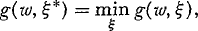
Two regions: A, conforming to the D-optimal designs not having D = 0 among its points, and B, conforming to the D-optimal designs, having D = 0 as a design point, are separated from each other. The parameters assumed are: IC₅₀ = 1, m = −1.5, D_max = 1000.

Figure 3 illustrates what happens to the D-optimal points when changes are made to one parameter at a time. The graph in the upper left corner of the figure conforms to E_con = 100, b = 10, IC₅₀ = 1, m = −1.5, D_max = 1000, λ = 1. The Hill curve in each of the 9 other panels uses all these values except one. This new quantity replaces the corresponding original value and is shown in the upper right corner of each panel. When the slope varies from a shallow one (m = −0.5) to a steep one (m = −10), the two middle D-optimal points tend to converge while staying on different sides (to the left vs. to the right) of >IC₅₀. This is illustrated by two panels in the left column, rows 2 and 3. When λ increases within a range such that the corresponding (λ, b/E_con) point belongs to the region B, Figure 2, then the two middle D-optimal points both tend to drift to the right while the distance between them decreases, as shown in the 2 panels in the top row. The 2 panels refer to λ = 0.6 and λ = 1.5, respectively. As soon as λ exceeds a certain value, all three D-optimal points except for the cap (D_max) move to the right. That happens when, for example, λ = 3 in our setting. The 4 other graphs (two of them conforming to b = 0.01 and b = 80, respectively, and two corresponding to D_max = 10 and D_max = 10000, respectively) are indicative of the effect that an increase in b alone or increase in D_max alone will have regarding the location of D-optimal points. As b decreases towards 0, the second D-optimal point moves to the right, and the third point moves even farther to the right. At b = 0, the third and fourth D-optimal points degenerate into one point at D_max. As D_max increases, the second and third D-optimal points move slowly to the right; the fourth point is always at D_max.

Figure 3.

Influence of changing parameters on 4 D-optimal design points. The values are changed one at a time starting with a graph in the upper left corner of the figure that conforms to E_con = 100, b = 10, IC₅₀ = 1, m = −1.5, D_max = 1000, λ = 1.

Along with the 4-point D-optimal design, we explored two five-point designs which we call design A and design B, respectively. We intended to create a more robust design by adding a fifth additional point. Design A consists of the four D-optimal points plus an additional one computed as a geometric mean of the two middle D-optimal points. Design B merely replicates one of the D-optimal points (dose2 in Table 1). When all of the assumed parameter values are the true ones, the D-efficiencies for the 3 designs are: 4-point D-optimal, 1.00; 5-point design B, 0.951, 5-point design A, varies from about 0.93 to 0.94, depending upon the set of true parameters.

Table 1.

D-optimal designs used in laboratory experiments^a

Drug	IC₅₀ (μM)	m	Dmax (μM)	dose2^b (μM)	dose3 (μM)	dose5 (μM)
TMTX	0.00895	−1.79	8.95	0.00790	0.0303	0.0155
MTX	0.0223	−2.74	22.3	0.0206	0.0495	0.0319
AG2034	0.453	−0.825	453	0.321	5.57	1.34
AG2032	0.0774	−3.49	77.4	0.0726	0.145	0.103
AG2009	111	−1.03	1500^c	54.2	377	142
AG337	0.468	−1.54	468	0.405	1.94	0.885
ZD1694	0.0429	−1.69	42.9	0.0376	0.156	0.0765

Assumed parameter values are: E_con = 1.70, b = 0.137, λ = 0.794.

Dose2 and dose3 are two middle points in the 4-point D-optimal design. Dose5 is the fifth point used in design A together with the 4 D-optimal points.

Dmax = 1500 has been used in this case because a concentration as high as Dmax = 111000 (1000 times the IC₅₀) was impractical.

D-optimal designs were used in real laboratory cell growth inhibition studies with each of seven anticancer drugs combined with the concentration of 78 μM of folic acid (FA) in the medium. Concentration-effect experiments were conducted in a 96-well plate growth inhibition assay (Levasseur et al., 1995). Briefly, exponentially growing HCT-8 (human ileocecal adenocarcinoma) cells were plated in wells with RPMI 1640 medium supplemented with 10% dialysed horse serum on day 0, treated on day 1 and incubated at 37°C in a 5% humidified atmosphere. Treatments were randomized on each plate. Cell growth was measured on day 5 with the SRB protein dye assay.

Methotrexate (MTX) and Trimetrexate (TMTX) are inhibitors of the enzyme, dihydrofolate reductase. Tomudex (ZD1694) is an inhibitor of thymidylate synthase, and was a gift from Zeneca Pharmaceuticals (Macclesfield, England). AG2032 and AG2034 (inhibitors of glycinamide ribonucleotide formyltransferase), AG2009 (inhibitor of aminoimidazolecarbox-amide ribonucleotide formyltransferase) and AG337 (inhibitor of thymidylate synthase) were gifts from Agouron Pharmaceuticals, Inc. (San Diego, CA).

Assumed true parameter values for D-optimal design calculations were taken from previously-completed concentration-effect experiments. For each previous experiment, A. was estimated by fitting (2), after logarithmically transforming both sides of the equation, with unweighted linear regression, to the variances and means of each set of replicates at each design point. Also, for each experiment the E_con, b, I₅₀ and m were estimated by fitting (1) to experimental data with iteratively-reweighted nonlinear regression, with weights equal to the reciprocal of the predicted effect raised to the power, 2λ. These assumed true parameter values, along with the calculated D-optimal design points, are displayed in Table 1.

RESULTS

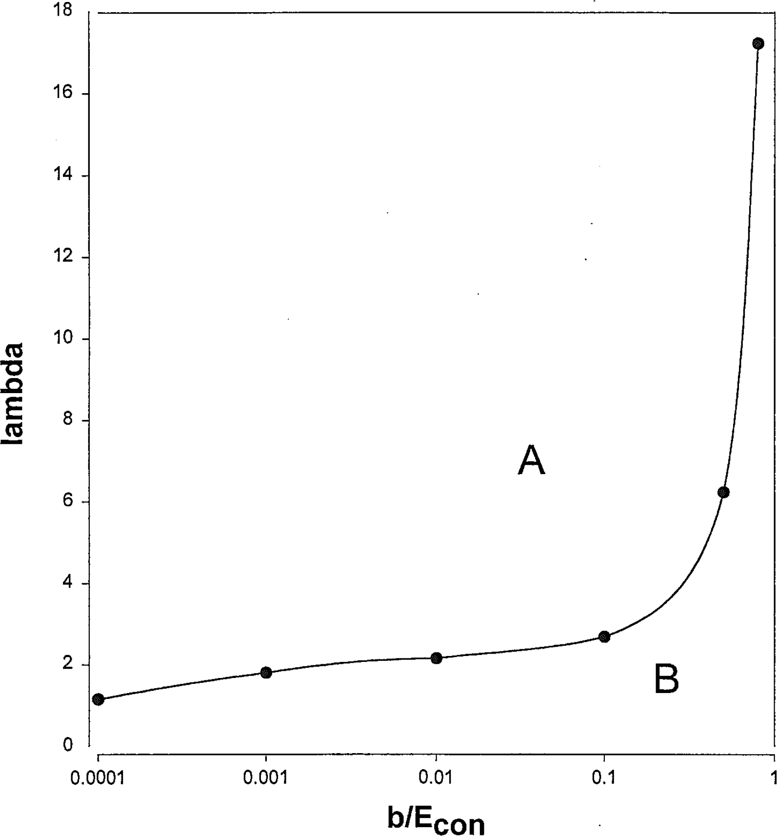
Table 2 gives the D-efficiencies of the 4-point D-optimal design, five-point design A, and a log-spread design, respectively, assuming that: (a) our prior estimates of the parameter values that we guessed to be the true ones were in fact the true values; or (b) the analysis of data from the log-spread design resulted in the true parameter values (although the actual design points are the same as in (a)). The 4-point D-optimal design included 1 control point at D = 0, and the dose2, dose3 and D_max points listed in Table 1. The 5-point design A included the extra dose5 point listed in Table 1 (the geometric mean of the dose2 and dose3 D-optimal points). The log-spread design included 1 control point at D = 0, and 11 concentrations serially-diluted by the factor $\sqrt{10}$ centered around the assumed IC₅₀. In case (a) the D-optimal design which yielded 100-percent D-efficiency is the clear winner, with 5-point design A being a close second with a D-efficiency of about 93% in all cases. [However, as noted above, the 5-point design B has a D-efficiency of 0.951 for all experiments in which the assumed parameter values are the true ones, and therefore, would have edged out the 5-point design A in this competition.] If assumption (b) is true, however, 5-point design A beats the 4-point D-optimal design in 9 out of 14 instances, including a dramatic difference in the case of the AG337 compound. Clearly, both 4-point D-optimal designs and 5-point designs proved themselves to be more efficient than log-spread designs.

Table 2.

D-efficiencies of a set of designs for anticancer drug concentration-effect curves

Drug	4-point D-optimal design	5-point design A	Log-spread design	4-point D-optimal design	5-point design A	Log-spread design
TMTX	1.00	0.936	0.728	0.987	0.952	0.678
MTX	1.00	0.936	0.775	0.885	0.933	0.569
AG2034	1.00	0.935	0.648	0.752	0.921	0.701
AG2032	1.00	0.936	0.747	0.878	0.851	0.587
AG2009	1.00	0.933	0.706	0.454	0.564	0.349
AG337	1.00	0.936	0.822	0.051	0.887	0.777
ZD1694	1.00	0.936	0.743	0.932	0.944	0.807

Note: Columns 2, 3, and 4 are D-efficiencies of 4-point D-optimal design, 5-point design A, and log-spread design, respectively, assuming that assumed parameter values were the true ones. Columns 5, 6, and 7 are D-efficiencies of corresponding designs assuming that log-spread design resulted in true parameter values.

For the real laboratory experiments, the 4-point D-optimal design included 10 replicates per design point, for a total of 40 data points per experiment; the 5-point design A included 10 replicates per design point for a total of 50 data points per experiment; and the 12-point log-spread design included 5 replicates per design point for a total of 60 data points per experiment. The estimates of the parameters needed to generate the D-optimal designs for these experiments were pooled from the results of extensive past studies conducted by our group on the same drug and cell line. The data for each of the 7 drugs for 3 designs (21 total experiments) were analyzed by fitting model (1) to data with iteratively-reweighted nonlinear regression as described above. The fitted concentration-effect curves for three compounds, MTX, TMTX, and AG2009, with 78 μM folic acid in the medium, for the 3 designs, are displayed in Figure 4. MTX is a representative example of a drug with a relatively steep concentration-effect curve, AG2009 has a very shallow curve, and TMTX has a curve with intermediate steepness. Note that for the log-spread design, for MTX only 1 design point is located on the falling part of the curve, for TMTX there are 3 points, and for AG2009 there are 5–7 points. Overall, the parameters were well estimated; the standard errors were around 10% or less of the parameter estimates. Exceptions include AG337 for the 4-point D-optimal design. For these 2 cases, the design points missed the falling portion of the concentration-effect curve. Overall, the corresponding parameter estimates are very similar among the 3 designs (Table 3) and the previous experiments.

Figure 4.

The fitted concentration-effect curves for three compounds, methotrexate, trimetrexate, and AG2009. Curves are displayed, along with the mean observed responses and standard deviations at the design points. Solid points represent observed data. Open triangles represent the predicted design points. Open squares represent control responses (always the first D-optimal design point).

Table 3.

Parameters estimated from laboratory experiments

Drug	Folic acid (μM)	IC₅₀(μM)	SE(μM)	m	SE	E _con	SE	b	SE
4-point D-optimal design
TMTX	78	0.0168	0.0015	–2.91	0.39	1.21	0.034	0.151	0.012
MTX	78	0.0295	0.0014	–3.50	0.30	1.20	0.033	0.147	0.011
AG2034	78	0.670	0.12	–1.01	0.11	1.24	0.040	0.175	0.015
AG2032	78	0.109	0.0048	–3.42	0.44	1.28	0.039	0.150	0.013
AG2009	78	306	48	–1.01	0.11	1.23	0.034	0.139	0.058
AG337	78	0.432	23	–8.87	6100	1.26	0.037	0.150	0.012
ZD1694	78	0.0447	0.0029	–2.33	0.28	1.26	0.036	0.175	0.013
5-point design A
TMTX	78	0.0147	0.00075	–2.56	0.23	1.23	0.035	0.153	0.012
MTX	78	0.0258	0.00099	–3.48	0.34	1.22	0.038	0.160	0.013
AG2034	78	0.465	0.059	–1.39	0.18	1.25	0.044	0.205	0.016
AG2032	78	0.106	0.0039	–3.18	0.36	1.28	0.039	0.149	0.013
AG2009	78	308	43	–1.09	0.18	1.23	0.032	0.150	0.048
AG337	78	0.519	0.025	–3.08	0.28	1.25	0.037	0.150	0.010
ZD1694	78	0.0427	0.0021	–2.81	0.27	1.26	0.035	0.185	0.011
Log-spaced design
TMTX	78	0.0124	0.00090	–1.99	0.23	1.23	0.017	0.172	0.013
MTX	78	0.0264	0.0014	–3.89	0.70	1.23	0.017	0.180	0.011
AG2034	78	0.596	0.058	–1.39	0.16	1.24	0.018	0.239	0.016
AG2032	78	0.114	0.0063	–3.26	0.45	1.24	0.018	0.171	0.011
AG2009	78	235	51	–0.959	0.16	1.24	0.018	0.185	0.076
AG337	78	1.36	0.089	–2.54	0.35	1.22	0.017	0.193	0.013
ZD1694	78	0.0628	0.0048	–2.20	0.32	1.24	0.018	0.184	0.019

Replication of design points is important in creating practical designs. It is known from theory (Bates and Watts, 1988; Seber and Wild, 1989) that the standard error of an individual parameter estimate decreases proportionally to $1 / \sqrt{n}$ , when n is large relative to the number of parameters in the model. Here n is the total number of design points used (each point is counted as many times as it is replicated). With the cell culture experimental system described above, where n was varied from around 10 to 100 for tine drugs, AG 2032 and AG 2009, for both D-optimal and several rival designs (data not shown), this theoretical result was confirmed. In addition, we showed that both 4-point D-optimal design and 5-point design A result in smaller standard errors of the parameter estimates if compared to logarithmically-spaced design. We have also showed that one needs to replicate tine 4 D-optimal points as evenly as possible in order to attain higher efficiency.

DISCUSSION

In this paper we examined different designs for the estimation of parameters in the Hill model. We assume that the true underlying model is known and that it is the Hill model. We also assume that the variance component is given by the power model (2). Our laboratory experience supports these assumptions. One should be aware that these assumptions may not hold for a different type of data. For instance, the binomial variance model σ²_i = y_i (1 — y_i) may be appropriate when data is quantal. It has also been used to model variance of continuous responses. This is a different model. The D-optimal designs for the logistic model with two parameters under binomial variance assumption were first derived by (Kalish and Rosenberger, 1978). The two D-optimal points conform in this case to the predicted responses of 0.176 and 0.824, respectively. Endrenyi and co-authors investigated how calculated designs depend on deviations from the correctness of different assumptions (Endrenyi et al., 1987). Their study concerns the logistic dose-response function with 2 parameters and the Hill model with 3 parameters. The authors consider effects of departure from 3 of the usual assumptions which are routinely made for the design of the experiments: (1) the form of the distribution and (2) the relative variances of the observational errors, and (3) the assumed prior knowledge of nonlinear parameter values. It has been shown that the D-optimal designs are sensitive with respect to the 3 types of departures albeit to a different degree: (1) and (2) affect both the location of the design points and the D-efficiency more dramatically than (3). “While we don't address the form of the distribution in the paper, we illustrate the departure from the two other assumptions in Figure 3 and provide relevant comments. It was shown that in this respect D-optimal designs are quite robust. The robustness improves when 5-point designs are considered. D-optimal designs, pure or modified, are practical and useful when the true underlying model is known, a good prior knowledge of parameters is available, and experimental units are relatively dear. A practical limitation of D-optimal designs, which we have encountered, centers at the relative ease in making serial dilutions of drugs in 96-well plate assays. Interestingly, when each experimental unit is very inexpensive, the extra time needed to make the appropriate drug dilutions to make a frugal D-optimal design may result in more trouble and expense than using less frugal serial-dilution-based logarithmically spread designs.

Both Mathematica code and a Fortran program to generate D-optimal designs for the Hill model are available from the authors, as are all derivations and proofs. Our software does not require initial guesses for D-optimal design points. We found that the more general ADAPT II (D'Argenio and Shumitsky, 1979) software package generated correct D-optimal designs for the 4-parameter Hill model for all cases in which the required initial design point guesses were reasonable.

References

Amisaki

, and Eguchi

(1999). A comparison of methods for estimating individual pharmacokinetic parameters. J Pharmacokinet Biopharm 27: 103–119.

Atkinson

A.C.

, and Donev

A.N.

(1992). Optimal Experimental Designs. Oxford University Press, New York.

Bates

D.M.

, and Watts

D.G.

(1988). Nonlinear Regression, Analysis and its Applications. John Wiley, New York.

Bezeau

, and Endrenyi

(1986). Design of experiments for the precise estimation of dose-response parameters: The Hill equation. J Theor Biology 123: 415–430.

Box

G.E.P.

, and Lucas

H.L.

(1959). Design of experiments in non-linear situations. Biometrka 46: 77–90.

D'Argenio

D.Z.

, and Schumitsky

(1979). Computer Programs in Biomedicine 9: 115–1134.

Davidian

, and Carroll

R.J.

(1987). Variance function estimation. J Am Stat Assoc 82: 1079–1091.

Endrenyi

Bezeau

M.L.

, and Jain

(1987). Optimal and robust design of experiments for the estimation of dose-response parameters. Am Statistical Assoc Proceedings of the Biopharm Section: 96–100.

Giltinan

D.M.

, and Ruppert

(1989). Fitting heteroscedastic regression models to individual pharmacokinetic data using standard statistical software. J Pharmacokinet Biopharm 17: 601–614.

10.

Holford

N.H.G.

, and Sheiner

L.B.

(1981). Understanding the dose-effect relationship: Clinical applications of pharmacokinetic-pharmacodynamic models. Clin Pharmacokinet 6: 429–453.

11.

Kalish

L.A.

, and Rosenberger

J.L.

(1978). Optimal designs for the estimation of the logistic function. Pennsylvania State Univ., Dept. Stat., Techn. Report 33.

12.

Levasseur

Faessel

Slocum

, and Greco

W.R.

(1995). Precision and pattern in 96-well plate cell growth experiments. Am Stat Assoc Proceedings of the Biopharm Section: 227–232.

13.

Levasseur

L.M.

Faessel

Slocum

H.K.

, and Greco

W.R.

(1998). Implications for clinical pharmacodynamic studies of the statistical characterization of an in vitro antiproliferation essay. J Pharmacokinet Biopharm 26: 717–733.

14.

Mannervick

(1982). Regression analysis, experimental error, and statistical criteria in the design and analysis of experiments for discrimination between rival kinetic models. Methods Enzymol 87: 370–390.

15.

Merle

, and Mentre

(1997). Stochastic optimization algorithms of a Bayesian design criterion for Bayesian parameter estimation of nonlinear regression models: Application in pharmacokinetics. Mathematical Biosciences 144: 45–70.

16.

Nash

J.C.

(1979). Compact Numerical Methods for Computers: Linear Algebra and Function Minimisation. John Wiley, New York.

17.

Sheiner

L.B.

, and Beal

S.L.

(1985). Pharmacokinetic parameter estimates from several least squares procedures: Superiority of extended least squares. J Pharmacokinet Biopharm 13: 185–201.

18.

Seber

G.A.F.

, and Wild

C.J.

(1989). Nonlinear Regression. John Wiley, New York.

Optimal Design for Estimating Parameters of the 4-Parameter Hill Model