Sage Journals: Discover world-class research

Abstract

The article considers the problem of characterizing the type of combined action produced by a mixture of toxic substances with the help of nonlinear response functions. Most attention is given to second-order models: the linear model with a cross-term and the quadratic model. General propositions are formulated based on the data on combined toxicity patterns previously obtained by the Ekaterinburg nanotoxicology team in animal experiments and analyzed with the help of the linear model with a cross-term. It is shown now that the quadratic model features these general characteristics in full measure, but interpretation of combined toxicity types based on isobolograms obtained by the quadratic model is more difficult. This suggests that where both models ensure a comparable quality of combined toxicity type identification, it would be enough to use the linear model with a cross-term.

Keywords

combined toxicity response surface methodology isobolograms nonlinearity

Introduction

Today, the response surface methodology (RSM) is one of the most important general methods used in the analysis of combined effects produced by mixtures of bioactive substances, including toxic ones.^1

-7 This method enables the potentialities of effective experimental design to be used for approximating a response function. Constructing such approximation requires choosing an analytical model whose parameters would be determined by fitting to experimental data.

The simplest way to approximate a response function is to construct a linear regression in relation to the doses of the toxic substances involved (hereinafter y will denote the response variable Y depending on the doses x_i of the toxicants X ₁, X ₂,…, X _n)

y = b_{0} + \sum_{i = 1}^{n} b_{i} x_{i} .

This model, however, is not adequate for identifying combined action types other than additivity. To allow for more complex types of combined toxicity, this model should include nonlinear terms or use explicitly nonlinear dependence models of a different analytical structure. At the same time, a model that is too complicated could overlook more essential patterns of change in the response with the dose.

The need for a trade-off between model complexity and interpretability has led to the recommendation that the model of choice for describing the nonlinear dependence of a response on influencing factors in the RSM should be one of the following two.^1
-3

The first one is the linear model with cross-terms, or the main effects model with interaction, given by the equation

y = b_{0} + \sum_{i = 1}^{n} b_{i} x_{i} + \sum_{i \neq j} b_{i j} x_{i} x_{j} + \dots + b_{12 \dots n} x_{1} x_{2} \dots x_{n} .

In this model, any possible nonlinearity of the response is allowed for by the introduction of cross-terms, that is, the products of the first-order independent variables.

The second model is different from model (1) in that it has higher order independent variables and is called an nth order polynomial model. The right-hand part of the equation that defines this model contains an nth order general polynomial in the variables x ₁, x ₂,…, x_n

y = b_{0} + \sum_{i = 1}^{n} b_{i} x_{i} + \sum_{i, j} b_{i j} x_{i} x_{j} + \dots \sum_{i} b_{i \dots i} x_{i}^{n} .

Both of these models are rather simple and, at the same time, sufficiently flexible tools for modeling nonlinear dose–response functions. In the general case, they may be used as a starting point for constructing the theoretical model of a response function. Note that each of these models includes as a special case the linear model, which, as noted above, expresses the additive nature of combined action.

Although these models may be defined for any number of influencing factors, it is practically possible to use them for describing the combined toxicity of 2 or 3 variables only. Indeed, functions with a large number of variables will contain, as a rule, products of variables with opposite signs. This would make it difficult to use such models for identifying combined action types. In such studies, researchers therefore tend to use models for 2 variables given by

y = b_{0} + b_{1} x_{1} + b_{2} x_{2} + b_{12} x_{1} x_{2}

for the main effects model with interaction, and

y = b_{0} + b_{1} x_{1} + b_{2} x_{2} + b_{12} x_{1} x_{2} + b_{11} x_{1}^{2} + b_{22} x_{2}^{2}

for the quadratic model (which may also be referred to as a “quadratic model with a cross-term”).

Since in the design of experiment theory, levels of factors are coded with integer numbers, using, for instance, the values 1 (controls), 0 (mean dose, if any), and +1 (maximum experimental dose of the toxic substance), then Equations 3 and 4 may be simplified when applied to certain types of experiment. For example, for an experiment with one 2-level factor and one 3-level factor, model (4) takes the form (assuming that the 3-level factor is coded with variable x ₁)

y = b_{0} + b_{1} x_{1} + b_{2} x_{2} + b_{12} x_{1} x_{2} + b_{11} x_{1}^{2} .

For a 3² full factorial experiment, the quadratic model (4) is applicable in its full form (with both variables squared). For an experiment with two 2-level factors, Equation 4 is reduced to Equation 3. In general, model (3) is the only possible nonlinear model for a 2² experiment.^8,9

One can obtain from Equations 3 or 4 approximations to single-factor dose–response functions by fixing the values of one of the variables. For instance, if the value of one of the factors has been fixed (eg, $x_{2} = x_{2}^{*}$ ), Equation 3 for the dependence of the response Y on the doses of the factor X₁ provides a linear equality (in relation to the dependence on x ₁)

y (x_{1}, x_{2}^{*}) = b_{0} + b_{2} x_{2}^{*} + x_{1} (b_{1} + b_{12} x_{2}^{*}) .

Doing the same for model (4) results in the quadratic dependence

y (x_{1}, x_{2}^{*}) = b_{0} + b_{2} x_{2}^{*} + b_{22} {(x_{2}^{*})}^{2} + x_{1} (b_{1} + b_{12} x_{2}^{*}) + b_{11} x_{1}^{2} .

Thus, in contrast to model (3), the presence of squared independent variables in model (4) leads to nonlinear approximations to single-factor dose–response functions.

Moreover, the presence of quadratic terms in model (4) can render this model essentially different from model (3) and give rise to additional difficulties for meaningful interpretation of combined toxicity analysis results obtained by means of this model. However, linear, quadratic, and more complex functions are broadly used in toxicological studies for approximating single-factor or multiple-factor dependence of the response on the doses of one or several toxicants.^10

-17 A promising approach to modeling of toxicological data is based on threshold models.¹⁸ Generally speaking, a single-factor dose–response dependence may be described by different models, and, as is stressed by the same authors,¹⁸ model selection is not a crucial issue. However, a multiple-factor dose–response function requires approximation by a function of the form (4) or a more complex one.

The uses of model (3) for 2 factors or the linear model with cross-terms (1) with n factors are sufficiently well presented in the literature. For instance, it is often used as the main model in the design of experiment for a mixture setting.^19
-21 Moreover, in experimental design employed for studying mixtures, the general polynomial model for n factors (2) is reduced to the canonical model (1) by virtue of the equality $x_{1} + x_{2} + \cdot + x_{n} = 1$ , where x ₁, . . , x_n in this case represent the fractional proportion of the components in the mixture.

In a series of publications,^{22

-36} model (3) was used by us for analyzing the combined toxicities of various substances. It was shown that this model enables one to describe both the unidirectional action types (additivity, subadditivity, superadditivity) and oppositely directed actions of toxic agents in a certain region of experimental dose combinations. Model (3) was also used for studying combinations of other toxic substances.³⁷ The properties of model (3) which are relevant to combined toxicity description were generally addressed in the studies.^8,9

The basic method for representing combined actions of toxic substances with the help of the response surface equation involves constructing response surfaces and sectioning them with constant-effect planes to obtain relevant lines. In toxicology, these lines (for 2 factors) or surfaces (for 3 and more factors) are called isoboles. The method of isoboles has been used for exploring joint action of toxic combinations in numerous studies carried out by other researchers as well.^{5,37

-51}

The shape of an isobole makes it possible to visually represent and distinguish such unidirectional combined toxicity types as additivity, subadditivity, and superadditivity (see Figure 1). The isobole for the additive action presents a straight line with regions of sub- and superadditive action on its sides.^5,39,41

-44 The distinctive feature of these lines is the presence of isoeffective doses for each toxicant, that is, each isobole crosses each of the coordinate axes at some point (with a positive coordinate). For the case of 2 variables, this means the presence of the points (D₁, 0) and (0, D₂), D₁ > 0, D₂ > 0 through which the isobole passes (see Figure 1).

Figure 1.

The general shapes of the isoboles for the unidirectional action of 2 factors: (A) additivity, (B) superadditivity, and (C) subadditivity.

However, even the application of such relatively simple functions as (3) and (4) often results in isoboles of a more complex shape. Below, we consider relevant examples. For the response function (3), the interpretation of such isoboles was considered in detail in the publications.^8,9,22,24,29 For model (4), this issue remains largely debatable.

When analyzing experimental data with the help of the model function (3), we discovered^{22

-36} some general principles, which were observed in all these experiments and which we believe to be representative of some important general patterns in combined toxicity, namely:

The combined toxicity type depends on the effect by which it is assessed.

The combined toxicity type depends on the choice of effect level.

The combined toxicity type depends on the dose ratio of the toxic agents in the combination.

Identification of the combined toxicity type in a certain region of dose combinations may reveal an opposite action of the toxicants.

Thus, it would be incorrect to draw any conclusion about the type of combined action of toxicants without specifying the effect, its level, and the dose combination involved. Only where the isobologram displays lines of the same type over the entire experimental range of doses could the type of combined toxicity demonstrated by the toxicants in relation to a given effect be stated unambiguously without specifying the level of this effect and the region of dose combinations. However, it is much more frequent to encounter cases where the combined toxicity type depends on both. Below, we show that these statements are true of the quadratic model (4) as well.

The Geometric Meaning of the Response Surfaces (3) and (4)

In considering models (3) and (4), it is useful to represent them as equations describing a certain surface in the space of the variables (x ₁, x ₂, y). Because both Equations 3 and 4 are second-order equations, they define second-order surfaces.^52,53 If we disregard the degenerate cases of these surfaces, then Equation 3 will describe only one surface, that is, a hyperbolic paraboloid all sections of which with horizontal planes are hyperbolas with perpendicular asymptotes (Figure 2A). A more general model (4) defines 2 possible response surfaces—a general hyperbolic paraboloid with a random arrangement of the asymptotes created by its horizontal sections, or an elliptic paraboloid^52,53 (Figure 2B).

Figure 2.

Nondegenerate response surfaces for models (3) and (4): (A) hyperbolic paraboloid; (B) elliptic paraboloid. The straight lines depict the coordinate axes.

Although they are very dissimilar, each of these surfaces can represent both the variants of unidirectional combined action (additivity, superadditivity, and subadditivity) and actions in opposite directions. At the same time, even where both model (3) and (4) define a hyperbolic paraboloid for some index, the resulting isoboles may be essentially different due to a more complex form of the response surface in model (4).

The distinctive features of models (3) and (4) may be seen if we consider the sections of these surfaces in Figure 3A and B, respectively, in the region containing their centerpoints (Figure 3). As can be seen from these figures, the presence of 2 asymptotes in models (3) and (4) in a case of a hyperbolic paraboloid results in an explicit division of the region of dose combinations into subregions, each of which features curves of a certain type. Changing from one region into another in an uninterrupted manner is impossible because the level lines cannot cross the asymptotes. However, the isobole for a given response level may consist of 2 lines located in different regions of dose combinations thus forming a composite curve.

Figure 3.

The general shapes of isoboles for surface (4): (A) the case of a general hyperbolic paraboloid; (B) the case of an elliptic paraboloid. The dashed lines show the asymptotes for the hyperbolas and the axes for the ellipses.

If surface (4) presents an elliptic paraboloid, its sections considered in the region containing the center form closed ellipses. Interpretation of these ellipses in the context of combined toxicity type identification presents a considerable difficulty.

Thus, in general where we come across such complicated curves as full hyperbolas for the model of hyperbolic paraboloid (3) or (4) or full ellipses for the model of elliptic paraboloid (4), it is necessary to divide the region of dose combinations into subregions to enable an unambiguous interpretation of the combined action type to be made in each of them. This prominent feature of complex isoboles will be illustrated by the experiments that we have carried out so far.

Examples of Isoboles for the Quadratic Model (4)

The examples presented in this section are based on the previously published experiments briefly described below.

Experiment (E1)

The results of this experiment were reported in the studies by Katsnelson et al,²⁶ Minigalieva et al,²⁷ and Katsnelson et al.³³ Stable suspensions of NiO and/or Mn₃O₄ nanoparticles (NPs) were administered to rats by intraperitoneal (IP) injection at a dose of 0.50 mg or 0.25 mg three times a week up to 18 injections, either separately or in different combinations. Thus, we obtained 9 groups of rats: (1) controls, and rats given (2) 0.50 mg NiO-NPs, or (3) 0.25 mg NiO-NPs, or (4) 0.50 mg Mn₃O₄-NPs or (5) 0.25 mg Mn₃O₄-NPs, or (6) 0.50 mg NiO-NPs + 0.50 mg Mn₃O₄-NPs, or (7) 0.25 mg NiO-NPs + 0.25 mg Mn₃O₄-NPs, or (8) 0.50 mg NiO-NPs + 0.25 mg Mn₃O₄-NPs, or (9) 0.25 mg NiO-NPs + 0.50 mg Mn₃O₄-NPs.

Experiment (E2)

The results of this experiment were reported in the study by Katsnelson et al.²⁸ Sodium fluoride solution was administered to rats by IP injection at a dose equivalent to 0.1 median lethal dose (LD₅₀) 3 times a week up to a total of 18 injections. Two-thirds of these rats and of the sham-injected ones were exposed to the whole body impact of a 25-mT static magnetic field (SMF) for 2 or 4 hours a day (note 1), 5 times a week. Thus we had 6 groups of rats: (1) controls (IP injections of normal saline); (2) rats administered sodium fluoride IP injections; (3) rats exposed to the SMF for 4 hours per day; (4) rats exposed to the SMF for 2 hours per day; (5) rats exposed to the SMF for 4 hours per day and fluoride IP injections; (6) rats exposed to the SMF for 2 hours per day and fluoride IP injections.

Experiment (E3)

The results of this experiment were reported in the study by Privalova et al.³⁰ Barium chromate (BaCrO₄) and manganese dioxide (MnO₂) fine powders were suspended in normal saline and instilled intratracheally into rat lungs separately or in combination at a dose of 5.0 or 2.5 mg in 1 mL of the suspension, while the control rats received 1 mL of normal saline only. Thus, we obtained 9 groups of rats according to each dose combination of the chemicals involved. Some cytological characteristics of a bronchoalveolar lavage fluid cell population of rats were assessed 24 hours after the intratracheal instillation.

Combinations of Harmful Factors Acting in the Same Direction

Cases of unidirectional action are well known and have long since been considered a basis for describing the combined action in any experiment.^{5,39,41
–43} Models (3) and (4) also enable one to describe just such cases. If the approximations (3) and (4) fit the experimental data well, the isoboles for these models will be qualitatively similar, though somewhat different in shape.

Consider the examples of unidirectional action isobolograms in Figure 4. Figure 4A demonstrates additivity in the combined action of SMF and NaF. Note that in experiment (E2), one factor (SMF) had 3 levels, including zero, while the other (NaF) only 2. The quadratic model (4) in this case was therefore reduced to a model with one-squared variable

Figure 4.

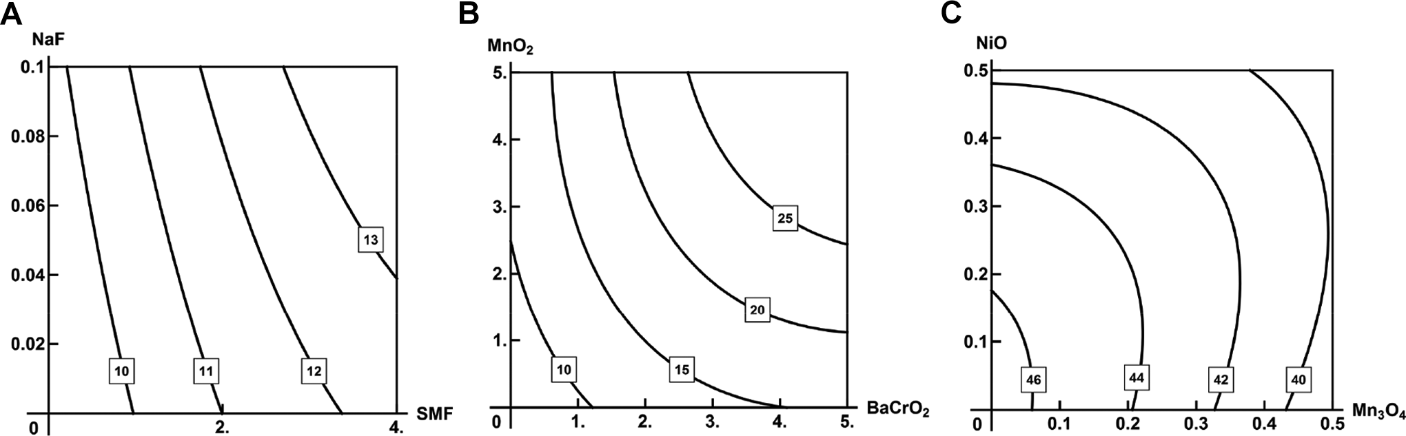
Unidirectional action isoboles in experiments (E1) to (E3). For each case, we have indicated the type of surface corresponding to Equation 4 for a given index. (A) Experiment (E2): hyperbolic paraboloid. Additivity for leukocytes in blood, 109/L.; (B) Experiment (E3): elliptic paraboloid. Superadditivity for the total number of particles engulfed by alveolar macrophages; (C) Experiment (E1): elliptic paraboloid. Subadditivity for the albumin content of blood serum, g/L. The boxes on the lines specify the levels of effect corresponding to a given isobole.

y = b_{0} + b_{1} x_{1} + b_{2} x_{2} + b_{12} x_{1} x_{2} + b_{11} x_{1}^{2},

where x ₁ represents SMF.

The use of nonlinear approximations, such as (3) or (4), for identifying the type of combined toxicity makes it necessary to estimate the degree to which resulting isoboles differ from a straight line. Figure 4A demonstrates just such a case. For Equation 3, a conclusion concerning the departure of the isobole from linearity may be drawn from the estimate of statistical significance of coefficient b ₁₂ for the product x ₁ x ₂. For approximation (4), a corresponding formula will be more complicated, as it will include also coefficients at the variables squared. However, in the case of Figure 4A, it is clear without any calculations that the isoboles should be regarded as straight lines. Thus, here, we deal with one and the same type of combined toxicity in all the range of experimental doses, namely, additivity.

We can describe in the same way the other 2 graphs in Figure 4. Similar examples can be provided for the other experiments of ours to which model (4) could be applied. Note in these cases that the type of combined action is the same over the entire region of dose combinations considered. In the majority of our experiments, however, the type varied depending on the response level or on the region of dose combinations.

The characteristic feature of unidirectional action isoboles is that they present graphs of decreasing functions. In other words, for maintaining the level of response with increasing the dose of one toxicant, it is necessary to reduce the dose of the other, that is, a decrease in the dose of one substance is compensated by an increase in the dose of the other. This compensation may be linear as in Figure 4A, or nonlinear as in Figure 4B and C, but in each of these cases the constancy of the effect is ensured by a balanced change in the doses of the substances—an increase in the dose of one of them should be compensated with a decrease in the dose of the other. Consequently, from the standpoint of isobole shape, a unidirectional action manifests itself as an isobole, which is a decreasing function graph. More specifically, if $Y (x_{1}, x_{2})$ is a response function, the isobole corresponding to effect Y ₀ is the graph of an implicit decreasing function defined by equality $Y (x_{1}, x_{2}) = Y_{0}$ .

However, in our experiments, we often came across situations where we failed to describe the behavior of the isoboles over the entire range of dose combinations in one way as, for example, in Figure 4. Moreover, we came across isoboles that represented increasing functions and, hence, did not describe the unidirectional action of the agents involved.

Combinations of Harmful Factors Acting in Opposite Directions

The concept of oppositely directed actions of toxicants is insufficiently considered in toxicological studies.⁵⁴ However, in the experiments of our team, this type of combined toxicity occurred rather frequently.^8,9,22,24,28 Its distinctive feature is that for maintaining the level of effect while increasing the dose of one toxicant, it is necessary to increase the dose of the other as well. Consequently, for an action in opposite directions, the isobole-defining function $Y (x_{1}, x_{2}) = Y_{0}$ will be an increasing one.

Note that the majority of effects feature action in opposite directions only in a certain subregion of dose combinations although some effects may display it over the entire region of experimental dose combinations as well. Although oppositely directed action is a special type of combined toxicity, it could be considered together with subadditivity. Indeed, in subadditivity, the substances mutually attenuate each other, and so in order to achieve the same level of effect as in additivity, it is necessary to increase the dose of at least one of the toxicants. The oppositely directed action of the toxicants is even more antagonistic in this respect. The oppositely directed action may therefore be called “explicit antagonism” unlike subadditivity, which may be called “implicit (hidden) antagonism.” Besides, when one analyzes the type of combined action by the shape and slope of the isobole, the segments of subadditive and oppositely directed action are often observed to be connected on the same curve.

In our experiments, we saw various cases of oppositely directed action, which showed themselves as ascending curves of different shapes. Nevertheless, we do not think it would be reasonable to additionally subdivide such rising isobole curves into various types.

Figure 5 shows isoboles for an oppositely directed action of 2 substances. In Figure 5A, an oppositely directed action of fluoride and SMF is seen over the entire region of experimental dose combinations. In Figure 5B, an oppositely directed action of Mn₃O₄ and NiO NPs in one region of dose combinations combines with canonical cases of unidirectional action (subadditivity and superadditivity, respectively) in the region between the asymptotes of the hyperbolas. Note also that the subadditivity in the region of low and medium doses of Mn₃O₄ and NiO transforms into an opposite action at higher doses of either of the substances. A similar picture can be seen in Figure 5C, but in this case, higher doses of both toxicants (MnO₂ and BaCrO₂ microparticles) display a superadditive combined action. In both cases in Figure 5B and C, the entire region of experimental dose combinations is divided into subregions, in which the type of combined toxicity is maintained the same. In both cases, this subdivision is affected by the asymptotes of the set of hyperbolas forming the isobologram.

Figure 5.

Isoboles for oppositely directed actions in experiments (E1) to (E3). In all these cases, surface (4) presents a hyperbolic paraboloid. (A) Experiment (E2): oppositely directed action over the entire range of dose combinations. Reduced glutathione in whole blood, µmol/L; (B) Experiment (E1): oppositely directed action with asymptotes subdividing the region of dose combinations. Subadditivity is observed for the low doses of both substances. The asymptote intersection point occurs in the region of experimental doses. Lymphocytes, %; (C) Experiment (E3): oppositely directed action with the asymptotes dividing the region of dose combinations. The asymptote intersection point occurs in the region of dose combinations. Number of internalized particles within one neutrophilic leukocyte. The boxes on the lines specify the levels of effect corresponding to a given isobole.

Composite Isobolograms for the Quadratic Model (4)

The division into subregions of one type of combined action depends essentially on the theoretical model used for representing the dependence of the response on the doses of the impacting factors. If several theoretical models are considered and each of these models fits experimental data well, the subregions of dose combinations with various types of combined toxicity predicted by such models will be qualitatively identical.

Let us consider some more examples of isobolograms in which the region of dose combinations is divided into subregions with certain types of combined action. If model (3) is used, the region is divided by the mutually perpendicular asymptotes of the hyperbola so that each subregion features only one type of combined action. For model (4), as we saw above, one of the possible response surfaces is also a hyperbolic paraboloid whose sections will be hyperbolas. The asymptotes present in the region of experimental dose combinations in this case also divide the region into segments, which should be analyzed separately. However, because the asymptotes of the hyperbolas in model (4) may intersect at any angle, the interpretation of the isoboles in this case will be more complicated. In particular, segments with different types of combined toxicity may occur together on the same line.

Figure 6 shows isobolograms for which the division of the region of dose combinations goes along the asymptotes of the hyperbolas resulting from the sectioning of surface (4) with constant-effect planes. In each subregion, the isoboles are arranged in about a similar pattern so that one such subregion displays combined toxicity of one certain type. For example, Figure 6A displays subadditivity at low levels of effect (the corresponding isoboles are located in the bottom left corner of Figure 6A). Proceeding into other regions of dose combinations (located between the asymptotes), we see isoboles of a completely different type. The interpretation of such isoboles depends on effect level. For example, for the isoboles that are close to the asymptotes of the hyperbolas (eg, for effect level 64,5), the combined toxicity is described as additive (at low doses of NiO), then changing into an oppositely directed action (at high doses of NiO). In general, it is obvious that such isobolograms cannot be unambiguously interpreted from the standpoint of combined toxicity type assessment.

Figure 6.

Composite isoboles featuring an oppositely directed action. In all cases, surface (4) is a hyperbolic paraboloid, and the point of intersection of the asymptotes occurs in the region of experimental dose combinations. (A) Experiment (E1): average RBC volume; (B) Experiment (E2): low-density lipoproteins; (C) Experiment (E3): percentage of degenerated alveolar macrophages. The boxes on the lines specify the levels of effect corresponding to a given isoboles. RBC indicates red blood cell.

Conclusions

Identifying the type of combined action in multiple factor toxicological studies presents a difficult problem. The reason is that the actual behavior of the response to a combined action of toxic agents may be ambiguous within the experimental region of dose combinations. Such behavior cannot be attributed to a particular model as its inherent feature. Rather, it is characteristic of the varied response of biological systems to a multifactorial impact in various dose combinations of the participating agents and the dependence of the combined action type on response level. Allowing for these circumstances leads to a more complex description of the type of combined toxicity, which, in particular, requires dividing the region of dose combinations into segments in which the type of combined action could be interpreted unambiguously. Such subdivision depends largely on the theoretical response model used, although it does not rule out a qualitatively similar picture of combined action as revealed by various models.

Moreover, the choice of a model for theoretical representation of the dependence of the response on the doses of the participating factors defines the shape of the line of constant response level (isobole) which may appear rather complicated even for a relatively simple response function model. For example, an isobole for one and the same level of response may appear consisting of the several segments located in different subregions of dose combinations with essentially different shapes. In other words, for the given level of response, the combined action is of different types depending on which region of dose combinations of the toxicants is considered.

Moreover, apart from the well-known classical types of unidirectional action isoboles representing additivity, subadditivity, and superadditivity, experiments may reveal isoboles whose shapes are considerably different from these types. Namely, the resulting complicated or composite isoboles may be explained by an oppositely directed action of the substances in some region of dose combinations. We define as oppositely directed combined action which requires increasing the doses of both toxicants for maintaining constant response. Such type of combined action can be called explicit antagonism. Depending on which effect is chosen for the analysis of combined toxicity, a given pair of substances may display various types of the latter including an oppositely directed one. However, most often an opposite action appears in only a certain subregion of the region of experimental dose combinations.

This variety of cases occur when one analyzes experimental data using even such simple models as the linear model with a cross-term (3) or the quadratic model (4). The basic difference of model (4) from model (3) consists in the presence of the squares of the independent variables in the former, the consequence of which is the possibility of a quadratic approximation for single-factor dose–response functions compared to linear functions for model (3). The latter may be applied as the basic one in a case where nonlinearity should be taken into account explicitly with no additional information on the shape of this nonlinearity being available. As is stated in “Experimental Design for Formulation”: “At the beginning of an investigation, and without prior subject-matter knowledge, one would have no idea about the functional relationship between the response and the mixture variables. What is often done at this point is to hypothesize a linear polynomial model, sometimes called a screening model .”¹⁹

When constructing a model for experimental data, the researcher has a wide choice of possible analytical representations for the response function and so should choose one, representing a compromise between the complexity of approximation and the possibility of interpreting the findings, which is made possible with simple model functions. As such a compromise, the RSM theory recommends models (3) or (4).^1,2,4 It is obvious that from the standpoint of combined toxicity type assessment, model (3) has the advantage that the shape of respective isoboles allows one to obtain a more simple and clear-cut interpretation of the combined action type. We maintain that in relation to the problem of combined toxicity type identification, the most important thing is to have basic qualitative characteristics, and these can be well obtained from the simpler model (3), provided it fits the available experimental data as well as model (4).

Thus, the analysis of toxicological experimental data for identifying the type of combined toxicity should start with the use of such relatively simple models as (3) and (4). There are standard tools for statistical verification of the quality of each of these models, which is a prerequisite for making an appropriate choice. For such a choice, it is useful to construct isobolograms for a given index (effect) in the region of experimental dose combinations. The shapes of these isoboles may be both classical (Figure 4) or more complicated (eg, Figures 5 and 6). A meaningful interpretation of complex isoboles is only possible by allowing for, firstly, the dependence of the type of combined toxicity on the chosen toxic effect; secondly, the chosen level of the effect; and thirdly, the ratio of the combined factors doses. It is essential for a correct interpretation of the isoboles to allow for the likelihood of an oppositely directed action of the toxic agents, which may be present together with any of the classical types of combined toxicity for the same level of effect. The quality of models (3) and (4) being comparable, preference should be given to model (3) because the interpretation of isoboles with this model is easier, and the qualitative picture of combined toxicity will be identical for both models.

Footnotes

Declaration of Conflicting Interests

The author(s) declared no potential conflicts of interest with respect to the research, authorship, and/or publication of this article.

Funding

The author(s) received no financial support for the research, authorship, and/or publication of this article.

Note

References

Box

GEP

Draper

. Response Surfaces, Mixtures and Ridge Analyses. 2nd ed. Hoboken, NJ: John Wiley & Sons Inc.; 2007.

Myers

Montgomery

Anderson-Cook

ChM

. Response Surface Methodology: Process and Product Optimization Using Designed Experiments. (Wiley Series in Probability and Statistics) . 4th ed. Hoboken, NJ: John Wiley & Sons Inc.; 2016.

Kappele

. Blind Analysis for Design of Experiments and Response Surface Methodology. Minitab Edition. Billingham, WA: CreateSpace Independent Publishing Platform; 2017.

Anderson

Whitcomb

. RSM Simplified: Optimizing Processes Using Response Surface Methods for Design of Experiments. 2nd ed. Hoboken, NJ: Productivity Press; 2016.

Greco

Bravo

Parsons

. The search for synergy: a critical review from a response surface perspective. Pharmacol Rev. 1995;47(2):331–385.

Khuri

, ed. Response Surface Methodology and Related Topics. Singapore: World Scientific Publishing Co. Pte. Ltd; 2006.

Nielsen

Østergaard

Larsen

. Toxicological Risk Assessment of Chemicals. A Practical Guide. New York, NY: Informa Healthcare USA, Inc.; 2008.

Panov

Varaksin

. Identification of combined action types in experiments with two toxicants: a response surface linear model with a cross term. Toxicol Mech Methods. 2016;26(2):139–150.

Panov

Varaksin

Minigalieva

Katsnelson

. The response surface methodology as an approach of choice to modeling and analyzing combined toxicity: theoretical premises, the most important inferences, experimental justification. Biom Biostat J. 2017;1(1):112.

10.

Gennings

Carter

Jr Carchman

Teuschler

Simmons

Carney

. A unifying concept for assessing toxicological interactions: changes in slope. Toxicol Sci. 2005;88(2):287–297.

11.

Hunt

. A regression spline model for developmental toxicity data. Toxicol Sci. 2006;92(1):329–334.

12.

Burgoon

Zacharewski

. Automated quantitative dose-response modeling and point of departure determination for large toxicogenomic and high-throughput screening data sets. Toxicol Sci. 2008;104(2):412–418.

13.

Forgacs

Ding

Jaremba

Huhtaniemi

Rahman

Zacharewski

. BLTK1 murine Leydig cells: a novel steroidogenic model for evaluating the effects of reproductive and developmental toxicants. Toxicol Sci. 2012;127(2):391–402.

14.

Thomas

Jenkins

Kaina

. Influence of DNA repair on nonlinear dose-responses for mutation. Toxicol Sci. 2013;132(1):87–95.

15.

Bell

Ives

Jonas

. Nonlinear effects of nanoparticles: biological variability from hormetic doses, small particle sizes, and dynamic adaptive interactions. Dose-Response. 2014;12(2):202–232.

16.

Lamm

Robbins

Chen

Goodrich

Feinleib

. Discontinuity in the cancer slope factor as it passes from high to low exposure levels—arsenic in the BFD-endemic area. Toxicology. 2014;326:25–35.

17.

Kienhuis

Slob

Gremmer

Vermeulen

Ezendam

. A dose-response modeling approach shows that effects from mixture exposure to the skin sensitizers isoeugenol and cinnamal are in line with dose addition and not with synergism. Toxicol Sci. 2015;147(1):68–74.

18.

Slob

Setzer

. Shape and steepness of toxicological dose-response relationships of continuous endpoints. Crit Rev Toxicol. 2014;44(3):270–297.

19.

Smith

. Experimental design for formulation. In: ASA-SIAM Series on Statistics and Applied Probability. Philadelphia, PA: SIAM. Alexandria, VA: ASA; 2005.

20.

Cornell

. A Primer on Experiments with Mixtures. Hoboken, NJ: John Wiley & Sons, Inc.; 2011.

21.

Peterson

Novick

. Nonlinear blending: a useful general concept for the assessment of combination drug synergy. J Recept Signal Transduct. 2007;27(2):125–146.

22.

Varaksin

Katsnelson

Panov

. Some considerations concerning the theory of combined toxicity: a case study of subchronic experimental intoxication with cadmium and lead. Food Chem Toxicol. 2014;64:144–156.

23.

Minigalyeva

Katsnelson

Privalova

. Toxicodynamic and toxicokinetic descriptors of combined chromium (VI) and nickel toxicity. Int J Toxicol. 2014;33(6):498–505.

24.

Panov

Katsnelson

Varaksin

. Further development of mathematical description for combined toxicity: a case study of lead–fluoride combination. Toxicol Rep. 2015;2:297–307.

25.

Katsnelson

Panov

Minigaliyeva

. Further development of the theory and mathematical description of combined toxicity: an approach to classifying types of action of three-factorial combinations (a case study of manganese-chromium-nickel subchronic intoxication). Toxicology. 2015;334:33–44.

26.

Katsnelson

Minigalieva

Panov

. Some patterns of metallic nanoparticles’ combined subchronic toxicity as exemplified by a combination of nickel and manganese oxide nanoparticles. Food Chem Toxicol. 2015;86:351–364.

27.

Minigalieva

Katsnelson

Privalova

. Attenuation of combined nickel(II) oxide and manganese(II, III) oxide nanoparticles’ adverse effects with a complex of bioprotectors. Int J Mol Sci. 2015;16(9):22555–22583.

28.

Katsnelson

Tsepilov

Panov

. Applying theoretical premises of binary toxicity mathematical modeling to combined impacts of chemical plus physical agents (A case study of moderate subchronic exposures to fluoride and static magnetic field). Food Chem Toxicol. 2016;95:110–120.

29.

Katsnelson

Panov

Varaksin

Minigalieva

Privalova

Sutunkova

. Changes in the dose–response relationship of one toxicant under simultaneous exposure to another toxicant. Dose-Response. 2016;14(4):1–9.

30.

Privalova

Katsnelson

Varaksin

Panov

Balesin

. The pulmonary phagocytosis response to separate and combined impacts of manganese (IV) and chromium (VI) containing particulates. Toxicology. 2016;370:78–85.

31.

Minigalieva

Katsnelson

Panov

. In vivo toxicity of copper oxide, lead oxide and zinc oxide nanoparticles acting in different combinations and its attenuation with a complex of innocuous bioprotectors. Toxicology. 2017;380:72–93.

32.

Minigalieva

Katsnelson

Panov

. Experimental study and mathematical modeling of toxic metals combined action as a scientific foundation for occupational and environmental health risk assessment. A summary of results obtained by the Ekaterinburg research team (Russia). Toxicol Rep. 2017;4:194–201.

33.

Katsnelson

Privalova

Sutunkova

. Experimental research into metallic and metal oxide nanoparticle toxicity in vivo. In: Yan

Zhou

Gardea-Torresdey

, eds. Bioactivity of Engineered Nanoparticles. 1st ed. Series: Nanomedicine and Nanotoxicology. Singapore: Springer Nature Singapore Pte, Ltd.; 2017:259–319.

34.

Minigalieva

Bushueva

Fröhlich

. Are in vivo and in vitro assessments of comparative and combined toxicity of the same metallic nanoparticles compatible, or contradictory, or both? A juxtaposition of data obtained in respective experiments with NiO and Mn₃O₄ nanoparticles. Food Chem Toxicol. 2017;109(pt 1):393–404.

35.

Minigalieva

Katsnelson

Privalova

. Combined subchronic toxicity of aluminum (III), titanium (IV) and silicon (IV) oxide nanoparticles and its alleviation with a complex of bioprotectors. Int J Mol Sci. 2018;19(3):E837.

36.

Sutunkova

Privalova

Minigalieva

Gurvich

Panov

Katsnelson

. The most important inferences from the Ekaterinburg nanotoxicology team’s animal experiments assessing adverse health effects of metallic and metal oxide nanoparticles. Toxicol Rep. 2018;5:363–376.

37.

Curcic

Buha

Stankovic

. Interactions between cadmium and decabrominated diphenyl ethers on blood cells count in rats—multiple factorial regression analysis. Toxicology. 2017;376:120–125.

38.

Euling

Gennings

Wilson

Kemppainen

Kelce

Kimmel

. Response-surface modelling of the effect of 5α-dihydrotestosterone and androgen receptor levels on the response to the androgen antagonist vinclozolin. Toxicol Sci. 2002;69(2):332–343.

39.

Loewe

. The problem of synergism and antagonism of combined drugs. Arzneimittelforschung. 1953;3(6):285–290.

40.

Loewe

. Antagonisms and antagonists. Pharmacol Rev. 1957;9(2):237–243.

41.

Berenbaum

. The expected effect of a combination of agents: the general solution. J Theor Biol. 1985;114:413–431.

42.

Berenbaum

. Isobolographic, algebraic and search methods in the analysis of multi-agent synergy. J Am Coll Toxicol. 1988;7:927–938.

43.

Berenbaum

. What is synergy? Pharmacol Rev. 1989;41(2):93–141.

44.

Calabrese

. Multiple Chemical Interactions. Chelsea, MI: Lewis Publishers; 1991.

45.

El-Masri

Reardon

Yang

. Integrated approaches for the analysis of toxicologic interactions of chemical mixtures. Crit Rev Toxicol. 1997;27(2):175–197.

46.

Cassee

Groten

van Bladeren

Feron

. Toxicological evaluation and risk assessment of chemical mixtures. Crit Rev Toxicol. 1998;28(1):73–101.

47.

Boedeker

Backhaus

. The scientific assessment of combined effects of risk factors: different approaches in experimental biosciences and epidemiology. Eur J Epidemiol. 2010;25(8):539–546.

48.

Tallarida

. Revisiting the isobole and related quantitative methods for assessing drug synergism. J Pharmacol Exp Ther. 2012;342(1):2–8.

49.

Jarvis

Thompson

. A golden approach to ion channel inhibition. Trends Pharmacol Sci. 2013;34(9):481–488.

50.

Foucquier

Guedj

. Analysis of drug combinations: current methodological landscape. Pharma Res Perspect. 2015;3(3):e00149.

51.

Hernandez

Gil

Lacasaña

. Toxicological interactions of pesticide mixtures: an update. Arch Toxicol. 2017;91(10):3211–3223.

52.

Berger

. Geometry. V II. Springer Verlag Berlin Heidelberg; 1987.

53.

Krivoshapko

Ivanov

. The second order surfaces. In: Encyclopedia of Analytical Surfaces. Springer International Publishing Switzerland. 2015: 613–626.

54.

Tallarida

Lamarre

Benamar

. Combinations of drugs that produce opposite effects. Int J Pure Appl Math. 2011;71(3):415–425.

Using Various Nonlinear Response Surfaces for Mathematical Description of the Type of Combined Toxicity

Abstract

Keywords

Introduction

The Geometric Meaning of the Response Surfaces (3) and (4)

Examples of Isoboles for the Quadratic Model (4)

Experiment (E1)

Experiment (E2)

Experiment (E3)

Combinations of Harmful Factors Acting in the Same Direction

Combinations of Harmful Factors Acting in Opposite Directions

Composite Isobolograms for the Quadratic Model (4)

Conclusions

Footnotes

Declaration of Conflicting Interests

Funding

Note

References