Sage Journals: Discover world-class research

Abstract

Using ABAQUS software as a tool and 225/60R18 tire as the research object, a finite element model of the tire was established and longitudinal slip simulation was conducted based on the completion of longitudinal slip and rubber material tests. By comparing the tire-pavement contact stress under longitudinal slip conditions with different angles of belt layers and the stress on the first belt steel cord, the influence of different angles of belt layers on the grounding characteristics of tires were analyzed. The results showed that under static loading conditions, the trend of tire-pavement contact stress presented a symmetrical “W” shape. Under dynamic longitudinal slip conditions, the tire-pavement contact stress curve was significantly different from the static loading simulation, with significant fluctuation and presented an irregular “W” shape, and asymmetric distortion occurred with the change of slip rate. At higher slip rates (±20%), the higher the asymmetry of the grounding imprint at the 61° and 63° belt layer angles. At the 65° belt layer angle, the ground imprint is more evenly distributed on the tread. The curve of stress variation on the belt steel cord along the path is in an “M” shape, and the stress on the belt steel cord is mainly distributed symmetrically on the tire-pavement contact surface corresponding to the tire shoulder position. The higher the slip rate, the higher the asymmetry of the stress distribution on both sides of the belt steel cord. At 65° and 67° belt angles, the distribution of grounding imprints on the tread are more uniform, and the tread is less prone to deformation, resulting in lower tread wear.

Keywords

Radial tire longitudinal slip belt layer tire grounding characteristics

Introduction

As the core structure of a radial tire, the belt layer is the main stressed component of the tire, and most of the damage to the tire occurs in the belt layer or at the end of the tire where stresses are concentrated in the rubber material.¹ The main function of the belt layer angle is to provide a certain degree of lateral rigidity to the tire tread, and its laying angle is an important factor in tire structural design. Tires may slip when braking or driving the vehicle, and the force on the tire at a certain slip rate is an important parameter that affects the driving performance of the vehicle and the degree of tread wear. Therefore, it is of great significance to study the dynamic grounding characteristics of tires under longitudinal slip conditions from the perspective of the belt layer. Li and Wang² analyzed the deformation and stress of belt ply’s steel wire under different forces through finite element simulation. Tian et al.^3,4 studied the radial tire cord stress in the dynamic state. Baranowski et al.^5,6 studied the strain rate of rubber materials. Phromjan and Suvanjumrat⁷ used finite element analysis to investigate tire material characteristics and tire dynamic performance. Liu et al.⁸ and Chen and Wu⁹ analyzed the effect of belt structure on tire tread imprint through a finite element model. Kucewicz et al.¹⁰ analyzed the stress distribution within the area of internal tire structures through the static radial deflection test. Ning et al.¹¹ and Sung et al.¹² respectively studied the effects of belt angle on the high-speed performance and lateral stiffness of tires. Lee¹³ and Feng and Yong¹⁴ respectively studied the effects of belt separation and belt angle on tire durability. Sun et al.¹⁵ and Ghoreishy¹⁶ respectively studied the effects of high-speed standing wave cord force and belt angle on tire rolling behavior. Baranowski et al.¹⁷ proposed a method to improve blast resistance of a tire by optimizing the angle of the cord. The above scholars have conducted some analysis on the different performance of tires from the perspective of the belt angle or the force of cord, but have not studied tires from the perspective of the belt layer angle under longitudinal slip conditions. In this study, the feasibility of the tire finite element model was verified based on the combination of tire longitudinal slip test and longitudinal slip simulation. Then, the finite element method was used for longitudinal slip simulation to analyze the tire-pavement contact stress and the stress on the first belt steel cord under different belt angles.

Methods

This paper used a combination of test and simulation methods to study the tire grounding characteristics. Firstly, tensile tests were conducted on the tire material to determine the selection of constitutive models, followed by finite element modeling of the tire. Based on the theory of tire longitudinal slip, the longitudinal slip test was conducted with the six-component force testing machine. The feasibility of the finite element model is verified by comparing the test results with the simulation results. Finally, based on the established tire finite element model, the influence of different angles of belt layers on tire grounding characteristics under longitudinal slip conditions was studied.

Longitudinal slip theory of radial tire

When the vehicle brakes, accelerates or turns, the tire tread in the grounding area will have obvious displacement relative to the road surface, which is called slip. According to different driving conditions, slip can be divided into lateral slip and longitudinal slip. The longitudinal force Fx is the force that moves forward in the x direction of the tire on the ground, providing acceleration and deceleration for the tire, as shown in Figure 1. Longitudinal slip test is a study of the relationship between tire slip and longitudinal force, simulating the braking and driving conditions of the tire on the ground. When the slip rate is positive, the wheels are in a driving state and the tires generate driving force; When the slip rate is negative, the wheels are in a braking state and the tires generate braking force. The slip rate formula is shown in equation (1), where ω is the angular velocity of the wheel center, ω₀ is the angular velocity of the straight free rolling wheel center.

S = \frac{(ω - ω_{0})}{ω_{0}}

(1)

Figure 1.

Schematic diagram of longitudinal force.

The Magic Formula model is a tire model that uses the combination of trigonometric functions to fit the tire test data. After obtaining the test data of slip rate, the data was fitted using the PAC2002 magicformula.¹⁸ The original formula is as follows:

y = D * \sin {C \tan^{- 1} [B x - E (B x - \tan^{- 1} B x)]}

(2)

{\begin{matrix} D = y_{p} \\ C = 1 \pm [1 - 2 \tan^{- 1} (y_{s} / D) / π] \\ B = \tan θ / (C D) \\ E = {B x_{p} - \tan [π / (2 C)]} / [B x_{p} - \tan^{- 1} (B x_{p})] \end{matrix}

(3)

where D is the peak value of the curve, C is the shape coefficient of the curve, which controls the sine function range of the Magic Formula, B is the tire stiffness coefficient, and E is the curvature parameter at the peak value of the curve, as shown in Figure 2.

Figure 2.

Curve of relevant parameters of the Magic Formula.

In the pure longitudinal slip experiment, the curve showed an asymmetric shape about the origin of coordinates. To offset the curve from the origin, we introduce a horizontal offset Sh and a vertical offset Sv. At this point, the Magic Formula becomes the following:

F_{x} = D * \sin {C \tan^{- 1} [B X_{1} - E (B X_{1} - \tan^{- 1} B X_{1})]} + S_{v}

(4)

where F_x is the longitudinal force, X1 is the independent variable of the combination of longitudinal forces, defined as X1 = S + Sh, S is the longitudinal slip ratio of the tire, and B, C, D, and E are the fitting coefficients of the Magic Formula, which were obtained by MATLAB fitting.¹⁹

Tire material test and tire finite element model

Tire material test

According to the different tire rubber materials, the tire was divided into 10 types: tread, belt layer, sidewall, Apex, inner liner, bead filler, carcass rebar, fetal crown layer, wing, and bead rubber. All rubber samples were standard samples after vulcanization. The material testing machine was used to conduct uniaxial tensile tests on various parts of the tire compound and extract corresponding stress-strain data. The rubber samples were processed into dumbbell shapes according to the standard GB/T-528, as shown in Figure 3. To avoid the impact of temperature on the test results, the rubber samples were placed at 25℃ for 24 h before the test.

Figure 3.

Tire material tensile test and rubber sample.

Rubber material is an approximately incompressible elastic body that requires a specialized constitutive model to be defined. ABAQUS software provides various rubber constitutive models, in this paper, three common constitutive models, Yeoh, Mooney-Rivlin, and Neo-Hooke, are selected for fitting. The data related to 10 tire compounds were obtained from the material tensile test in Figure 3. In this paper, the main deformation is concentrated in the tread grounding area, so the tread rubber is taken as the basis for selecting the constitutive model. As shown in Figure 4, Yeoh model was found to have the best fitting effect after considering the range of strain rate variation of tire rubber material. Therefore, Yeoh constitutive model was selected to characterize the mechanical properties of rubber materials.²⁰ The strain energy density expression of the Yeoh model is as follows:

W_{Y e h o} = C_{10} (I_{1} - 3) + C_{20} {(I_{1} - 3)}^{2} + C_{30} {(I_{1} - 3)}^{3}

(5)

Figure 4.

Constitutive model fitting.

In the formula, C₁₀ is positive, reflecting the initial shear modulus, and C₂₀ is negative, indicating that the rubber material softens when it is moderately deformed. C₃₀ is positive, which can show the hardening phenomenon of rubber during large deformation. I1 is the strain invariant.

It is necessary to consider the viscoelasticity and damping of the tire material during the rolling process. Described the viscoelastic material of the tire using the Prony series in material identification using Abaqus software. The shear modulus can be expressed as gi = 0.6. The bulk modulus can be expressed as ki = 0. Other relevant parameters are represented as tau-i = 0.1. The keyword expression of this parameter in Abaqus software is as follows:

*VISCOELASTIC, TIME=PRONY **Viscoelastic parameters

*0.6,0.0,0.1

In the Abaqus software solver, the damping type of the tire uses the Beta damping in Rayleigh damping. The volume viscosity is represented by *BULK VISCOSITY, and the keyword expression of this parameter in Abaqus software is as follows:

*DAMPING, BRTA=1E-7 **Damping parameters

*BULK VISCOSITY **Volume viscosity

*0.06,1.2

The fitting parameters of the Yeoh model for the 10 types of rubber are shown in Table 1.

Table 1.

Yeoh model parameters of different rubber compounds.

Rubber type	C₁₀(MPa)	C₂₀(MPa)	C₃₀(MPa)
Tread	0.669470	0.036176	−0.000420
Belt layer	1.602325	0.063284	−0.001573
Sidewall	0.382588	0.014033	−0.000091
Apex	2.965836	−0.164619	0.010994
Inner liner	0.495442	0.000405	0.00001
Bead filler	1.061872	0.060687	−0.000922
Carcass rebar	0.87901	0.054067	−0.001014
Fetal crown layer	0.857678	0.040701	−0.000274
Wing	0.66047	0.036176	−0.00042
Bead	1.626822	0.1774	−0.009939

Establishment of tire finite element model

In order to reduce the number of meshes and improve quality of meshes, the tire finite element model was simplified under reasonable conditions. Set the rim to an analytical rigid body. Embedded rebar units are used in the simulation of the belt layer and the carcass layer.²¹ The skeleton material was embedded into the tire through the *embedded command. The triangular element of rubber material adopts CGAX3H (3-node, bilinear, twisted, hybrid solid element) axisymmetric element, while the quadrilateral element of rubber material adopts CGAX4H (4-node, bilinear, twisted, hybrid solid element) axisymmetric element. The rebar element adopts the surface element SFMGAX1 (2-node, linear, twisted, axisymmetric membrane element).

Based on the above analysis of the tire rubber material, the tire could be roughly divided into the tread, belt layer, Apex, bead, lining layer, and other relevant parts. Firstly, based on the geometric structure and dimensions of the tire, a two-dimensional cross-sectional model of the tire was drawn using AutoCAD software and imported into Abaqus software in iges format. The tire sections were divided into corresponding Set using Abaqus software and assigned with corresponding material properties.²² And then the half section of the tire was reflected into a complete section by the Reflect command in Hypermesh software. Finally, a complete three-dimensional tire was generated by using the *SMG (SYMMETRIC MODEL GENERATION) command to rotate 50 layers in the circumferential direction. At this time, the element types of rubber material were C3D6H and C3D8H three-dimensional elements, and the rebar element type was SFM3D4R surface element. The established tire model is shown in Figure 5. The first belt layer was 61° to the meridian direction, the second belt layer was −61° to the meridian direction, and the crown belt was 90° to the meridian direction. The three-dimensional model had 35,800 nodes and 32,000 grid cells.

Figure 5.

Establishment of finite element model.

Longitudinal slip test and simulation

The longitudinal slip test was conducted on a 225/60R18 tire with a belt angle of 61° using the MTS six-component force testing machine as shown in Figure 6. The slip range was set to −20% ~ 20%, and the tire pressure was set to 0.26 MPa. The speed was set to 60 km/h, and the load was set to 6300 N. The tire was placed on the spindle of the test bench, and a fixed speed ω was given to the tire by a drive motor connected to the wheel hub. The vertical hydraulic column exerted a radial force on the tire to make the tire contact with the steel strip shown in Figure 6. The steel strip was supported by two internal drums. The tire is given a fixed rotational speed ω and, at the same time, the drum is given an angular velocity ω₀ with respect to the hub center. The purpose was to generate a speed difference and achieve slip. The speed of the tire during the test was monitored by sensor in real time to keep the slip rate between −20% ~ 20%. The data measured by the testing machine were scattered points at various time points. The raw data was fitted using the PAC2002 magic formula. The fitted test data is shown in the black curve in Figure 11.

Figure 6.

Six-component force testing machine.

Longitudinal slip simulation is shown in Figure 7. The longitudinal slip simulation used an analytical rigid plate to simulate the ground, and the tire position was fixed in the whole process. The simulation process was divided into four analysis steps: inflating, loading, rotating, and slipping. The tire inflation process was simulated by applying a pressure of 0.26 MPa to the inner liner layer. In the loading analysis step, the process of the tire pressing the ground was simulated by reverse loading of the ground. In the rotation analysis step, the steady-state transport analysis was used to calculate the rolling process of the tire. And the tire is given a fixed speed ω to make it roll forward. In the slipping analysis step, the isometric amplitude curve was used to fit the slip rate from −20% to 20%. When the tire model rolled freely on the ground, a differential speed ω₀ was given to simulate the condition of tire longitudinal slipping. The above method was used to simulate the tire model under different belt angle conditions, the fitted simulation data is shown in red in Figure 11(b).

Figure 7.

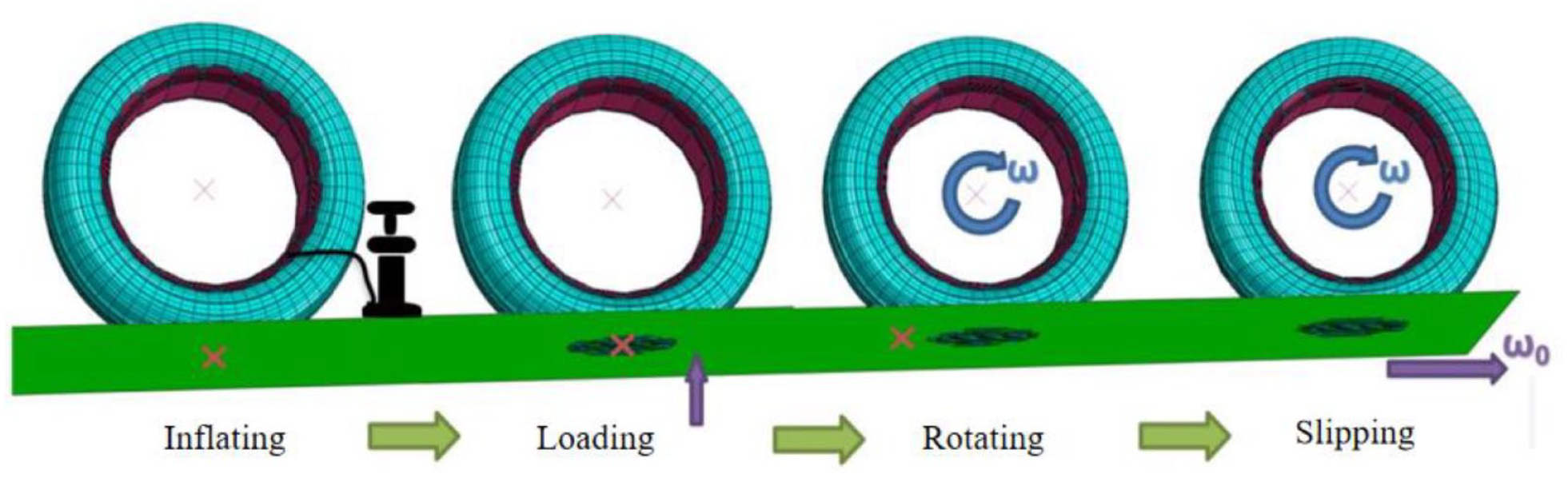
Simulation process of tire longitudinal slip.

Radial stiffness test was carried out with UKEN UP-2092 tire comprehensive testing machine as shown in Figure 8. The tire is mounted on the spindle of the testing machine, the four corners of the load-bearing platform are equipped with sensors sensing displacement and force, which can accurately measure the change of displacement and reaction force of the tire during the test. The PL2000 software of the computer host can control the whole test and extract the corresponding test data.

Figure 8.

UKEN UP-2092 tire comprehensive testing machine.

The radial stiffness G_z of the tire under vertical load can be expressed as:

G_{Z} = \frac{d F_{z}}{d_{z}}

(6)

In the formula, F_z is the radial force, and z is the radial displacement.

The tire pressure was set to 0.26 MPa and the load was set to 6300 N. Figure 9(a) shows the radial stiffness test of tire, the relationship between radial displacement and radial force can be obtained by analyzing and processing the test data. Figure 9(b) shows the tire radial stiffness simulation. The establishment of the simulation model is consistent with the loading analysis steps mentioned above. The test fitting results are shown in Figure 10. The red curve is the test data, and the blue curve is the simulation data. It can be seen from Figure 10 that the radial displacement of the tire increases with the increase of the radial force. The simulation curve fluctuates up and down with the test curve, and the deviation error is less than 10%.

Figure 9.

(a) Radial stiffness test and (b) Radial stiffness simulation.

Figure 10.

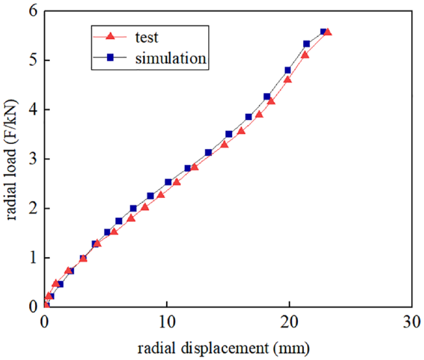
Radial stiffness test and radial stiffness simulation.

The fitting results of longitudinal slipping test and simulation are shown in Figure 11, the black curve represents the fitted test data. Under driving and braking conditions, the longitudinal force distribution of tires under the same load is uneven. Figure 11(a) shows the comparison between the test data and the simulation data before fitting, the simulation curve fluctuates with the test curve in the range of −20% to 20% slip rate. The simulation curves fluctuate drastically due to the large model grid, but the overall change trend is obvious. Using curves fluctuate drastically due to the large model grid, but the overall change trend is obvious. Using Origin software to perform median filtering on curves. Figure 11(b) shows the comparison between test data and simulation data after fitting. Under longitudinal slipping conditions, changes in the angle of the belt layer will not cause changes in the longitudinal force. The simulation and test results maintain good consistency, and the deviation error is within 10%. The established tire finite element model is effective.

Figure 11.

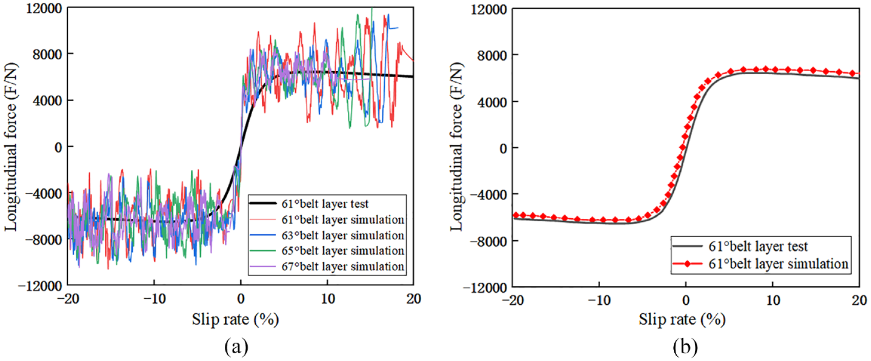
Comparison of longitudinal slip test and simulation: (a) comparison of test and the simulation before fitting and (b) comparison of test and the simulation after fitting.

Simulation analysis of tire grounding characteristics

The complex working condition of longitudinal slipping leads to the complex energy change inside the rubber. The pure longitudinal slipping test cannot observe the stress of the inner structure of the tire. Therefore, ABAQUS software was used to simulate and analyze the stress of each structure inside the tire. In this paper, longitudinal slip simulations with slip rate from −20% to 20% were carried out by changing the belt angle (61°, 63°, 65°, 67°), and the simulation results of the tire-pavement contact stress and the force on the first belt steel cord were analyzed. A uniform path was chosen for data analysis for models with different belt layer angles. The tire-pavement contact stress path and the stress path of the first belt steel cord are shown in Figure 12. In the tire-pavement contact stress path diagram, “Path of CPRESS” indicates the normal stress path of the contact surface (tire to ground). In the first belt steel cord stress path diagram, “Start” and “End” indicate the start and end points of the simulation path of the belt steel cord. The “α” indicates the angle of the belt layer.

Figure 12.

The tire-pavement contact stress path and the stress path of the first belt steel cord.

Analysis of tire-pavement contact stress

The stress on the path node of the tread grounding area in the loading analysis step is extracted for fitting. In the loading analysis step, the tire was in static state, which was used to simulate the static grounding mechanical test of tire. The stress variation is shown in Figure 13.

Figure 13.

Path diagram of static grounding stress.

It can be seen from Figure 13 that the change trend of tire-pavement contact stress is symmetrical “W” shape. Before the tire slip, the 61° belt angle curve had a relatively high grounding stress, but it can be almost ignored, that is, the change of belt angle had little impact on the static grounding stress. Under loading conditions, the tire-pavement contact stress corresponding to the tire tread position of the tire is the highest, reaching a maximum of 0.57 kN. The stress change trend on both sides of the tire tread is gentle.

The stress in the grounding area of tire in the rolling process is complex, so the stress and energy of slip rate at instantaneous time (−20%, −10%, 0%, 10%, 20%) are selected for research. The stress of all grid nodes on the tire-pavement contact stress path in Figure 12 is extracted, and the belt angle is changed for fitting, as shown in Figure 14.

Figure 14.

Distribution of tire-pavement contact stress at different angles of the belt layer.

It can be seen from the Figure 14 that the change of tire-pavement contact stress under different belt angle is obvious, the maximum can reach 0.33 MPa and the minimum is not less than 0.17 MPa. As the angle of the belt layer increases, the tire-pavement contact stress under braking condition shows a trend of decreasing, then increasing, and then decreasing, and the tire-pavement contact stress under driving condition shows a trend of increasing, then decreasing, and then increasing. The maximum tire-pavement contact stress under braking condition occurs at the 65° belt angle, the maximum tire-pavement contact stress under driving condition occurs at the 63° belt angle, and the increase in tire-pavement contact stress under driving condition is more pronounced than under braking condition. The belt angle was changed and the slip rate was determined to explore the change rule of tire-pavement contact stress on the path under various working conditions. The stress cloud and the trend of tire-pavement contact stress variation on the path nodes are shown in Figure 15.

Figure 15.

Tire-pavement contact stress cloud and path diagram for different belt layer angles under fixed slip rates. (a) −20% slip rate, (b) −10% slip rate, (c) 0 slip rate, (d) 10% slip rate, and (e) 20% slip rate

It can be seen from the tire-pavement contact stress cloud that the higher tire-pavement contact stresses occur at the 65° and 67° belt layer angles for braking conditions and at the 61° and 63° belt layer angles for driving conditions. This is similar to the stress variation pattern in Figure 11. At higher slip rates (±20%), the higher the asymmetry of the grounding imprint at the 61° and 63° belt layer angles. At the 65° belt layer angle, the ground imprint is more evenly distributed on the tread. It can be seen from the stress path diagram that the changes in tire-pavement contact stress at path nodes under different belt layer angles are complex, which is greatly different from static loading simulation. The fluctuations of tire-pavement contact stress at different belt layer angles are significant. During the dynamic longitudinal slipping process, the change in the angle of the belt layer has a significant impact on the tire-pavement contact stress. The trend of the tire-pavement contact stress changes in an irregular “W” shape, and asymmetric distortion occurs with the change in slip rate. At the slip rate of −20%, the 61° belt layer curve fluctuates violently and occurs severe asymmetric distortion, the maximum tire-pavement contact stress under the angle of the belt layer can reach 0.45 MPa. At the slip rate of −10%, the maximum value of tire-pavement contact stress appears in the 65° belt layer curve, the maximum tire-pavement contact stress under the angle of the belt layer can reach 0.4 MPa. At 0 slip rate, the braking condition gradually shifts to the driving condition, and the fluctuation of the tire-pavement contact stress curve is relatively small. Under this condition, the tire-pavement contact stress is mostly concentrated at 0.3 MPa. At the 10% slip rate, the maximum tire-pavement contact stress occurs in the 63° belt layer, the maximum tire-pavement contact stress can reach 0.45 MPa. And it is more obvious at the 20% slip rate, the maximum tire-pavement contact stress in the 63° belt layer can reach 0.68 MPa, and the tread is most prone to wear at this time.

Analysis of the stress on the belt steel cord

The values on the specified path nodes of the belt layer shown in Figure 12 were extracted, and the belt layer angle was changed for fitting, as shown in Figure 16.

Figure 16.

Distribution of the stress on the belt steel cord at different belt layer angles.

In Figure 16, the stress on the belt steel cord in the tire-pavement contact area increases with the increase of the belt layer angle. During the process of changing the slip rate from −20% to 20%, the average force on the belt steel cord changes more sharply at 61° and 67° belt layer angles, with a maximum stress of 33 N and a minimum force of no less than 18 N. The maximum stress on the belt steel cord under braking conditions occurs at the 67° belt layer angle, and the maximum stress on the belt steel cord under driving conditions occurs at the 65° belt layer angle. When the braking and driving conditions occur alternately, the stress on the belt steel cord changes obviously, and the stress cloud is shown in Figure 17.

Figure 17.

Stress cloud of belt steel cord with different belt layer angles at fixed slip rates. (a) −20% slip rate, (b) −10% slip rate, (c) 0 slip rate, (d) 10% slip rate, and (e) 20% slip rate

The highest Rebar stress in the stress of the belt steel cord can be seen that the stress on the belt steel cord increases with the increase of the belt layer angle, and the growth trend is obvious. There is a significant difference in the stress of the belt layer between the braking and driving conditions. The higher the slip rate, the higher the asymmetry of stress distribution on both sides of the belt steel cord. The stress on the belt steel cord under braking conditions is mainly concentrated at the “End” point of the path. When the slip rate gradually changes from −20% to 20%, the stress concentration area moves toward the “Start” point, and when the slip rate reaches 20%, the stress concentration area almost completely reaches the vicinity of the “Start” point. The variation pattern of stress concentration is shown in Figure 18.

Figure 18.

The belt steel cord stress path diagram under different belt layer angles. (a) 61°, (b) 63°, (c) 65°, and (d) 67°

Figure 18 shows the change of concentrated stress on the belt steel cord. At different belt layer angles, the variation trend on the “Start-End” path is obvious, and the entire curve shows an “M” shape. In the slip rate range of −20% to 20%, the curve changes from “low left to high right” to “high left to low right,” and the stress in the belt steel cord is mainly distributed symmetrically on the tire-pavement contact surface corresponding to the tire shoulder position. On the path, the maximum stress in the 61° belt layer can reach 55 N, and it can reach 63 N at 63° belt layer. The maximum stress in the 65° belt layer can reach 70 N, and in the 67° belt layer, the maximum stress can reach 72 N. Which effectively verifies that the stress increases with the increase of angle.

Conclusions

In this paper, based on the longitudinal slip theory, the tire longitudinal slip tests were conducted, and then the tire material tests were conducted to obtain relevant parameters. Based on these parameters, a corresponding tire finite element model was established in ABAQUS software. By comparing the longitudinal slip test and longitudinal slip simulation under the same working condition, it was found that the variation pattern was consistent, verifying the accuracy of the tire finite element model under dynamic working conditions. Finally, the analysis of the tire-pavement contact stress and the analysis of the stress on the first belt steel cord were carried out by changing the angle of the belt layer in the dynamic longitudinal slip simulation. The following conclusions were drawn:

(1) Under static loading conditions, the trend of tire-pavement contact stress changes in a symmetrical “W” shape. The tire-pavement contact stress corresponding to the tire tread position of the tire is the highest, reaching a maximum of 0.57 kN, and the stress change trend on both sides of the tire tread is smooth. The change of belt angle had little impact on the static grounding stress. Under dynamic longitudinal slipping conditions, there is a significant difference in the variation of tire-pavement contact stress at the path node compared to static loading simulation. The tire-pavement contact stress fluctuates greatly at different belt layer angles, with an irregular “W” shape and asymmetric distortion with the change of slip rate.

(2) During the process of tire dynamic slip, the maximum tire-pavement contact stress under braking condition occurs at the 65° belt angle, the maximum tire-pavement contact stress under driving condition occurs at the 63° belt angle, and the increase in tire-pavement contact stress under driving condition is more pronounced than under braking condition. At higher slip rates (±20%), the higher the asymmetry of the grounding imprint at the 61° and 63° belt layer angles. At 65° belt layer angle, the ground imprint is more evenly distributed on the tread.

(3) In the analysis of the stress on the belt steel cord, the stress on the belt steel cord in the tire-pavement contact area increases with the increase of the belt layer angle. The higher the slip rate, the higher the asymmetry of stress distribution on both sides of the belt steel cord. The stress on the belt steel cord under braking conditions is mainly concentrated at the “End” point of the path. When the slip rate gradually changes from −20% to 20%, the stress concentration area moves toward the “Start” point, and when the slip rate reaches 20%, the stress concentration area almost completely reaches the vicinity of the “Start” point. The curve of stress variation on the belt steel cord along the path is in an “M” shape, and the stress in the belt steel cord is mainly distributed symmetrically on the tire-pavement contact surface corresponding to the tire shoulder position.

(4) At 65° and 67° belt angles, the distribution of grounding imprints on the tread are more uniform, and the tread is less prone to deformation, resulting in lower tread wear.

Footnotes

Acknowledgements

Not applicable

Declaration of conflicting interests

The author(s) declared no potential conflicts of interest with respect to the research, authorship, and/or publication of this article.

Funding

The author(s) disclosed receipt of the following financial support for the research, authorship, and/or publication of this article:

1. Science and Technology Research Project of Xiamen University of Technology (No. YKJ22013R)

2. Research Project of Xiamen University of Technology (No.XPDKT20026)

3. Natural Science Foundation of Fujian Province (No. 2020J01276, No. 2023J011435)

4. Natural Science Foundation of Xiamen (No.3502Z20227217)

Availability of data and materials

The datasets used and analyzed during the current study are available from the corresponding author on reasonable request.

ORCID iDs

Jun-Ling Meng

Lu-Wen Chen

References

Huang

Meng

, et al. Finite element optimization design of the belt cord of the 235/45R18 tire. Rubber Ind 2020; 67(03): 209–213.

Wang

The finite element analysis of steel cord in radial tire’s belt ply. Key Eng Mater 2012; 501: 495–499.

Tian

Wang

, et al. A study on the viscoelastic behaviors of tire cords using dynamic mechanical analysis. J Eng Fiber Fabr 2020; 15(81): 1–7.

Tian

Wang

Wei

Study on dynamic mechanical properties of a nylon-like polyester tire cord. J Eng Fiber Fabr 2019; 14(6): 1–7.

Baranowski

Janiszewski

Małachowski

Tire rubber testing procedure over a wide range of strain rates. J Theor Appl Mech 2017; 55(2): 727–739.

Baranowski

Malachowski

Mazurkiewicz

Numerical and experimental testing of vehicle tyre under impulse loading conditions. Int J Mech Sci 2016; 106: 346–356.

Phromjan

Suvanjumrat

Material characteristic for capability analysis of solid tire by finite element method. Key Eng Mater 2018; 777(1): 416–420.

Liu

Ming

Jie

, et al. Effect of belt structure on footprint, radial stiffness and noise of PCR tire. Tire Ind 2011; 31(9): 534–536.

Chen

Effect of belt structure on the impression and braking performance of high-speed car radial tire. Tire Ind 2011; 31(9): 525–533.

10.

Kucewicz

Baranowski

Małachowski

Airless tire conceptions modeling | simulations. In: Proceedings of the 13th international scientific conference, 2017, pp.293−301. Cham: Springer.

11.

Ning

Jiang

Zhou

, et al. Effect of belt angle on high-speed performance of PCR tire. Tire Ind 2020; 40(4): 216–218.

12.

Sung

Kim

, et al. A study on characteristics of PRAT and cornering due to the belt angle of tire by the FEM. J Korean Soc Precis Eng 2006; 23(2): 104–112.

13.

Lee

Kim

Sung

, et al. A study on the fatigue life prediction of tire belt-layers using probabilistic method. J Mech Sci Technol 2013; 27(3): 673–678.

14.

Feng

Yong

Finite element optimization design of 12R22.5 tire belt cord. Elastomer 2021; 31(04): 29–99.

15.

Sun

Huang

Zhou

, et al. Experiment and analysis of cord stress on high-speed radial tire standing waves. Shock Vib 2019; 2019(3): 1–9.

16.

Ghoreishy

MHR

. Finite element analysis of steady rolling tyre with slip angle: effect of belt angle. Plast Rubber Compos 2006; 35(2): 83–90.

17.

Baranowski

Małachowski

Mazurkiewicz

Ł.

Local blast wave interaction with tire structure. Def Technol 2020; 16(3): 520–529.

18.

Shang

Wang

Analysis of tire dynamic characteristics based on PAC2002 magic formula. J Beijing Univ Inf Technol 2019; 34(06): 76–81.

19.

Kuiper

Van Oosten

JJM

. The PAC2002 advanced handling tire model. Veh Syst Dyn 2007; 45: 153–167.

20.

Zhou

Chen

, et al. Study on the influence of different tire cord structures on tire grounding characteristics. J Eng Fibers Fabr 2022; 17: 15589250221138549.

21.

Feng

Xie

Finite element analysis of radial tire based on ABAQUS. Times Automob 2019; (18): 124–126.

22.

Yao

Ground behavior analysis of tire based on ABAQUS modeling. Ningbo University, 2016.

Supplementary Material

Please find the following supplemental material available below.

For Open Access articles published under a Creative Commons License, all supplemental material carries the same license as the article it is associated with.

For non-Open Access articles published, all supplemental material carries a non-exclusive license, and permission requests for re-use of supplemental material or any part of supplemental material shall be sent directly to the copyright owner as specified in the copyright notice associated with the article.

0.00 MB

0.02 MB

Study on the influence of belt angle on tire grounding characteristics under longitudinal slip conditions

Abstract

Keywords

Introduction

Methods

Longitudinal slip theory of radial tire

Tire material test and tire finite element model

Tire material test

Establishment of tire finite element model

Longitudinal slip test and simulation

Simulation analysis of tire grounding characteristics

Analysis of tire-pavement contact stress

Analysis of the stress on the belt steel cord

Conclusions

Footnotes

Acknowledgements

Declaration of conflicting interests

Funding

Availability of data and materials

ORCID iDs

References

Supplementary Material