Sage Journals: Discover world-class research

Abstract

Based on the static resistive network investigated in Part 1 of this series, the resistive network model of the weft-knitted strain sensor with the plating stitch is explored under the elongation along course direction, and it changes with the conductive loops’ configuration and contact situation. Since the voltage is applied at both ends of the course, under a specific stretching state, the resistive network model can be reduced to a resistance network connected in series in the course direction and parallel in the wale direction, which determines that the sensor’s equivalent resistance increases with the growth of the conductive wale number, and decreases with the raise of the conductive course number. Through experiment and model calculation, it can be obtained that in the initial stage of stretching, the contact resistances’ changes are the main factors affecting the mechanical–electrical performance of the sensor. Then as the sensor is further stretched, the length-related resistances of the conductive yarn segments begin to affect the sensor’s properties due to yarns’ slippage and self-elongation. In addition, the weft jacquard plating technology makes the strain of the sensor reach about 32% before yarns’ slippage and self-elongation, which expands the sensor’s measurable strain range, and avoids irreversible deformation of the sensor after repeated use in this range. It can be verified that the sensor’s gauge factor can be improved by reducing the conductive course number and increasing the conductive wale number. It should be noted that the ground yarn will reduce the gauge factor of the sensor during stretching, so it is necessary to choose a ground yarn with a smaller fineness than the conductive face yarn and good elasticity in practical.

Keywords

Resistive network model weft-knitted strain sensor plating stitch elongation gauge factor mechanical–electrical analysis jamming contact resistance interlocking contact resistance length-related resistance

Introduction

Conductive knitted fabrics can be used as flexible strain sensors for limb movement and physiological parameter monitoring.^1–7 Some researchers have analyzed the influence of the fabric parameters of knitted sensors on their sensing performance through experiments.^7–14 These studies can intuitively tell us the empirical results, but they lack theoretical support. Exploring the mechanical–electrical properties of the knitted strain sensors, especially the changes law of the internal resistive network under their working, is the key to helping us understand their sensing principles and provides a benefit to design and optimize sensors for different scenarios. Some scholars have examined the mechanical–electrical performance of conductive knitted fabrics in both theoretical and experimental aspects. Zhang¹⁵ and Zhang et al.¹⁶ investigated the mechanical–electrical properties of two overlapped conductive yarns and the weft plain knitted strain sensor in unidirectional stretching separately. Li et al.^17,18 established the functional relationship between the tensile force and equivalent resistance of the conductive knitted fabrics compared with the results obtained in the unidirectional tensile experiments. Wang et al.^19,20 theoretically deduced the connection between the tensile force and equivalent resistance of elastic plain knitted fabric during the stretching process verified through experiments. Xie et al.²¹ also combined the experiments to confirm the relationship between the tensile force and the equivalent resistance of the conductive knitted fabric under biaxial stretching.

In the above surveys, the resistances involved are divided into contact resistance generated by the interlocking of the conductive yarns and length-related resistance. In practical applications, the weft plating technology is often adopted^{1,2,4,6,8,11–13,22} to increase the repeatability and stability of the sensor. The conductive yarn is used as the face yarn and the insulated elastic yarn used as the ground yarn in the sensing area. This plating stitch brings the new kind of contact resistance by the jamming of the conductive loops and the resistance dynamically varies in real-time during the deformation of the sensor. In the initial stage of tensile deformation in the course direction, the yarn segments, especially the needle loop and sinker loop, are straightened from the arc without slip. Simultaneously, the interlocking and jamming contact resistances are the main factors influencing the resistance change by rearranging the internal resistive network connections. As the stretching progresses, there exist the slippage and elongation of the segment yarn, causing the variations of the involved resistors in the resistive network. However, the existing mechanical–electrical analysis obviously cannot fully explain the working principle of compact weft-knitted strain sensors. Atalay et al.⁷ designed a sensor with only one course in the sensing area. They discussed the sensor’s resistance change mechanism during stretching, highlighting the impact of jamming contact resistance. Nevertheless, this method actually ignored the interlocking contact resistance. Once the conductive loop is worn or contaminated, the performance of the sensor will be significantly affected.

So, the existing models rarely fully regarded the rearrangement and variations of various resistors in the resistive network model of knitted strain sensors under the deformation along course direction. In Part 1 of this series,²³ the resistive network model of the weft-knitted strain sensor with the plating stitch under static relaxation has been studied. This article continues to explore the corresponding equivalent resistive network model under the elongation along course direction through observing the changes in the configuration of the conductive loop and the contact situation between the conductive yarns. The established model fully examines various contact resistances and length-related yarn resistance and notices that the elastic ground yarn probably makes the interlocking contact resistance disappear. Finally, experiments are performed to verify the correctness and usability of the new model and analyze the relationship between the gauge factor and the conductive loop course and wale numbers of the strain sensors to provide theoretical support for subsequent design and preparation of sensors suitable for different applications.

Loop configurations and resistance distributions under deformation

Figure 1 exhibits the changes in the conductive loop configurations and the jamming contacts between the loops of the weft-knitted strain sensor with the plating stitch during the stretching along course direction. Herein the resistance distributions are depicted with three stages due to the variations in the loop shape as the following:

In Initial State, the resistive network includes the jamming contact resistance RC₁, RC₂, and RC₄ (referring to the static relaxation in Part 1²³);

In Second State, the resistive network contains the jamming contact resistances RC₁ and RC₄;

In Final State, the resistive network only consists of the jamming contact resistance RC₄.

The arrangement of the yarn segments divided by the contact point where the contact resistance is located can also be seen from Figure 1. The corresponding length resistances are 0.5RL_{1_1}, RL_{1_2}, RL_{2_1}, RL_{2_2}. and RL₃. Moreover, RL, RL₁, and RL₂ are the length resistances of the total loop, needle loop, and sinker loop respectively. The relationship among these length-related resistances are expressed as

{\begin{cases} R L = R L_{1} + R L_{2} + 2 R L_{3} \\ R L_{1} = R L_{1_1} + 2 R L_{1_2} \\ R L_{2} = 2 (R L_{2_1} + R L_{2_2}) \end{cases}

(1)

The relative spatial position of the ground and face yarn mostly affects the contact of the conductive yarn of the face yarn in the interlocking point, as shown in Figure 2, which determines whether the interlocking contact resistance RC₃ is present. Hence two resistive network models are supposed to be established, with one involving RC₃ and the other not.

Figure 1.

Loop configurations and resistance distributions, containing the Front Side and Reverse Side, of the weft-knitted strain sensor with the plating stitch during the stretching along course direction: (a and b) Initial State, (c and d) Second State, and (e and f) Final State.

Figure 2.

Isolating impacts of the ground yarn on the conductive face yarn at the interlocking points during the elongation along course direction, which determine the existence of RC₃: (a) Initial State, (b) Second State, and (c) Final State.

Establishment and calculation of the resistive network models under deformation

The resistive network models in Initial State refer to those established and solved in Part 1.²³ The following focuses on exploring the resistive network models in Second State and Final State.

From now on, it should be noted that M and N mean the number of conductive loop course and wale in the conductive region separately. The contact resistances involved in the resistive network are first divided equally to the branches connected to them, which have been used by other scholars.¹⁸

Resistive network model containing RC₃

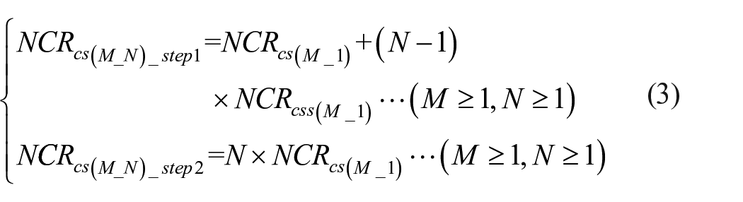
Existing models have proved that when the voltage is loaded in the course direction, the resistive network is a series of resistances.^18,19 Hence in this article, according to the arrangement rule of the conductive loops along the course direction, the resistive network model is first simplified into a series circuit in the course direction, as depicted in Figure 3. A simplified Second State resistive network composed of N-RC₁-wale and RC₁-wale is obtained by exchanging the conductive areas P₁ and P₂ (see Figure 3(a)). It obviously can be seen that the resistive network of Final State composed of N identical N-RC₁-wale (see Figure 3(b)). Equation (2) is the relationship between the total and local voltage during the simplification. Assuming NCR_cs _{(M_N)_step1} and NCR_cs _{(M_N)_step2} are the total equivalent resistance of the respective resistive networks of the two stages, NCR_cs _{(M_1)} and NCR_css _{(M_1)} are the equivalent resistances of N-RC₁-wale and RC₁-wale separately, then equation (3) can be obtained by Ohm’s law.²⁴

{\begin{cases} U = U_{1} + (N - 1) \times U_{2} \\ U = N \times U_{3} \end{cases}

(2)

{\begin{cases} N C R_{c s (M_N)_s t e p 1} = N C R_{c s (M_1)} + (N - 1) \\ \times N C R_{c s s (M_1)} \dots (M \geq 1, N \geq 1) \\ N C R_{c s (M_N)_s t e p 2} = N \times N C R_{c s (M_1)} \dots (M \geq 1, N \geq 1) \end{cases}

(3)

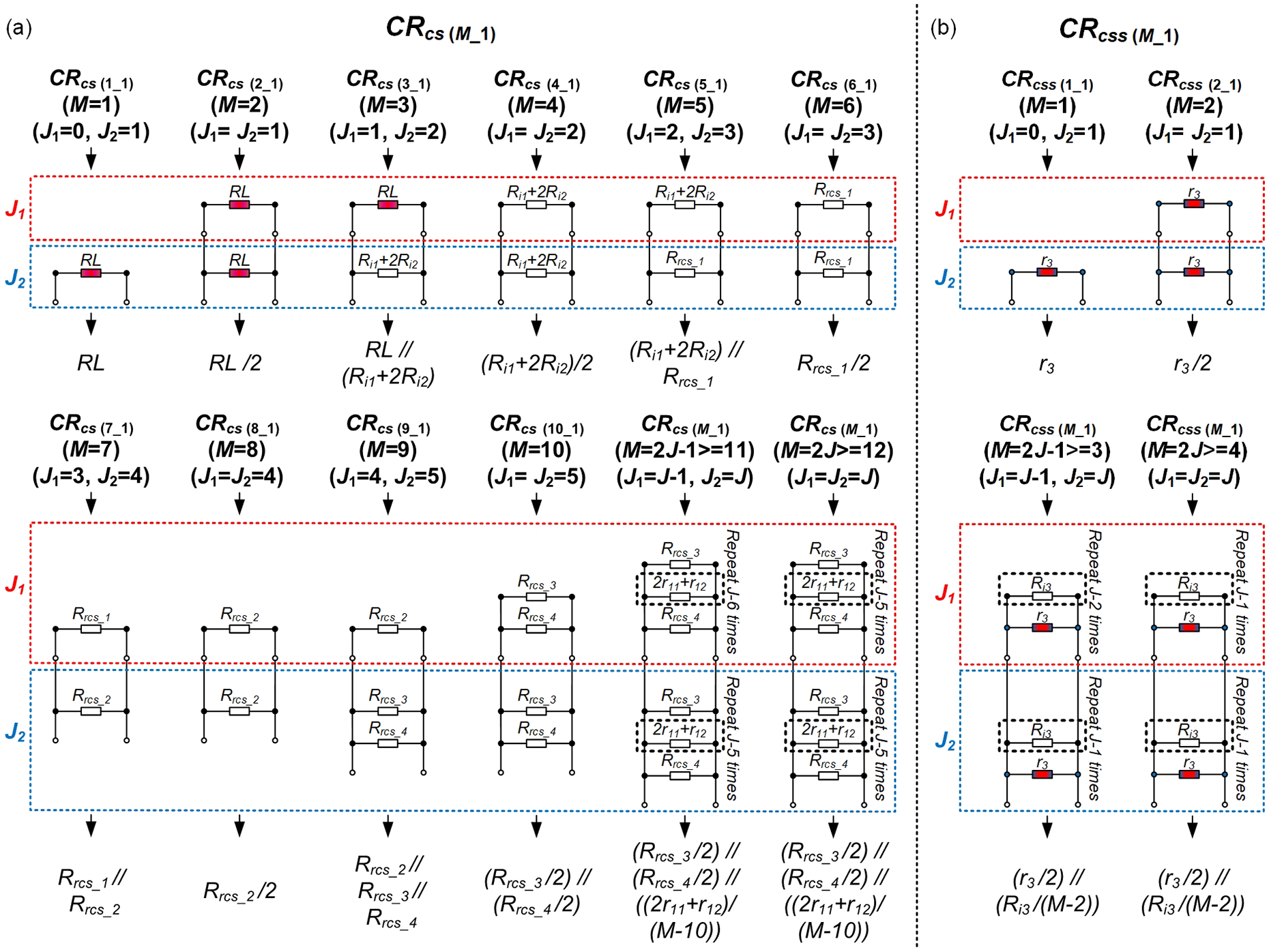
By Supplementary Theoretical Calculation 1, the final equivalent resistive circuits of NCR_cs _{(M_1)} and NCR_css _{(M_1)} with different M and their corresponding equations can be summarized in Figure 4, where the symbol “//” indicates the parallel of resistances. A series of equivalent transformations (Supplemental Figures S1–S7) was used to simplify the resistive network during the calculation, such as evenly dividing the contact resistors into the branches connected to themselves,¹⁸ splitting the nodes on the symmetry line, the merge of equipotential points, the four-terminal star to four-terminal network and the Y-Δ transformations,²⁴ the nodal analysis,²⁴ the series-parallel rule of resistance,²⁴ and removing the bridge resistors in the generalized Wheatstone Bridge.¹⁸ So far, the theoretical calculations of NCR_cs _{(M_N)_step1} and NCR_cs _{(M_N)_step2} with different M and N can be summarized as equations (S21) and (S22) in Supplemental Material, respectively.

Figure 3.

Simplifications of the weft-knitted sensor’s geometrical models in Second State and Final State, when voltage is applied to both ends of the course direction: (a) Step1: Second State and (b) Step2: Final State.

Figure 4.

Final equivalent resistive circuits of NCR_cs _{(M_1)} and NCR_css _{(M_1)} with different M and their corresponding formulas: (a) NCR_cs _{(M_1)} and (b) NCR_css _{(M_1)}.

Resistive network model ignoring RC₃

The resistive network model established in this section does not regard the interlocking contact resistance RC₃ due to overlooking the conductive face yarn’s isolation at the interlocking point caused by the elastic ground yarn.

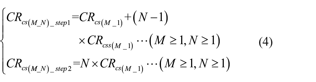
First, according to the simplified method in Figure 3, CR_cs _{(M_N)_step1} and CR_cs _{(M_N)_step2} represent the total equivalent resistance of the network models in Second State and Final State, CR_cs _{(M_1)} and CR_css _{(M_1)} indicate the equivalent resistances of N-RC₁-wale and RC₁-wale respectively, so the relationship between these resistances can be described as

{\begin{cases} C R_{c s (M_N)_s t e p 1} = C R_{c s (M_1)} + (N - 1) \\ \times C R_{c s s (M_1)} \dots (M \geq 1, N \geq 1) \\ C R_{c s (M_N)_s t e p 2} = N \times C R_{c s (M_1)} \dots (M \geq 1, N \geq 1) \end{cases}

(4)

Secondly, it should be noted that the different internal courses are only connected by RC₄ in this resistive network model, making the entire resistive network composed of two sub-resistive networks in parallel. Assuming that J₁ and J₂ are the number of courses within the two sub-resistive networks, their values depend on the number of course M of the entire resistive network. Moreover, since the two sub-resistive networks change in the same pattern with the number of internal courses, J is used to indicate J₁ and J₂. Here the relationships among J₁, J₂, J, and M can be deduced as equation (5), which means that the values of J₁ and J₂ are different with a difference of one when M is an odd number and are the same when M is an even number. In the following, CR_Jcs _{(J_1)} and CR_Jcss _{(J_1)} are used to signify the equivalent resistances of N-RC₁-wale and RC₁-wale of the sub-resistive network, respectively.

{\begin{cases} {\begin{cases} J_{1} = \frac{M - 1}{2} = J - 1 \\ J_{2} = \frac{M + 1}{2} = J \end{cases} \begin{matrix} \dots \end{matrix} (M = 2 J - 1 \geq 1, J \geq 1) \\ {\begin{cases} J_{1} = \frac{M}{2} = J \\ J_{2} = \frac{M}{2} = J \end{cases} \begin{matrix} \dots \end{matrix} (M = 2 J \geq 2, J \geq 1) \end{cases}

(5)

CR_cs _{(M_1)} and CR_css _{(M_1)} with the specific M can be solved by Supplementary Theoretical Calculation 2. Some equivalent transformations (Supplemental Figures S1 and S8–S11) are used, for example, evenly dividing the contact resistances into connected branches,¹⁸ the merging and rearrangement of the equipotential points, the nodal analysis,²³ removing the bridge resistors in the generalized Wheatstone Bridge,¹⁸ and the series-parallel rule. Moreover, the final equivalent resistive circuits of CR_cs _{(M_1)} and CR_css _{(M_1)} with different M and their corresponding equations can be concluded in Figure 5, revealing the relationships between CR_cs _{(M_1)} and CR_Jcs _{(J_1)}, CR_css _{(M_1)} and CR_Jcss _{(J_1)}. So far, the theoretical calculation of CR_cs _{(M_N)_step1} and CR_cs _{(M_N)_step2} with different M and N can be deduced as equations (S48) and (S49) in Supplemental Material separately.

Figure 5.

Final equivalent resistive circuits of CR_cs _{(M_1)} and CR_css _{(M_1)} with different M and their corresponding formulas: (a) CR_cs _{(M_1)} and (b) CR_css _{(M_1)}.

Experiment and model calculation

Materials prepared

Employing the weft jacquard plating technology in Part 1,²³ 111dtex silver-plated nylon filament as the conductive yarn was used as the face yarn in sensing area whose resistivity ρ and diameter d are 571.5 Ω/m and 0.1596 × 10⁻³ m respectively. In contrast, 86dtex low-elastic nylon yarn as the normal insulated yarn was used as the face yarn in the non-sensing area, and the same ground yarns in the two areas are 44dtex/33dtex nylon/spandex covered yarn. All strain sensors were prepared on SANTONI SM8 TOP2 MP seamless knitting machine with gauge 28 under the same process parameters with the samples prepared in Part 1.²³

Measurements of the strain along course direction in different tensile states

Using the method described in Supplementary Experiment 1, the strain along course direction (referred to ε in Figure 6) in different tensile states can be gauged. As shown in Figure 6, the variations of the jamming contact resistances during the loop deformation along course direction were further subdivided into the following stages: Initial State including contact resistances RC₁, RC₂, and RC₄, Second State containing Second State_1 and Second State_2 having contact resistances RC₁ and RC₄ and Final State involving only contact resistance RC₄.

Figure 6.

The Enlarged conductive loop configurations of the sensor, containing the Front Side and Reverse Side, in different tensile states with the corresponding strain ε: (a and b) Initial State, (c–f) Second State, and (g and h) Final State.

Then, during the elongation, it can be concluded that when ε is in the range of 0% to 10.8720%, the resistive network model refers to those of Initial State, hence the static relaxation resistive network model established in Part 1 can be used.²³ When ε is separately in the ranges of 10.8720% to 31.8443% and 31.8443% to 93.3445%, the resistive network models are consistent with those of the Second State and Final State.

Mechanical–electrical performance testing

The numbers of course and wale in the sensing area are considerable factors affecting the mechanical–electrical properties of the knitted strain sensor, so the conductive course numbers of the samples were designed to be 4, 10, and 14 differently while the conductive wale numbers were 50, 100, and 150 respectively.

The testing set (see Supplemental Figure S14) and method for the mechanical–electrical performance were depicted in Supplementary Experiment 2. The reason why 0% to 10% was selected as the strain range was to combine the initial empirical numerical values of each resistance obtained in Part 1²³ to calculate and probe the factors that affect the resistance value in this range. It is assumed that the yarn cross-section is always round, and the fiber arrangement within the yarn is unchanged. It can be seen from Figure 6 and Table S1 in Supplemental Material that the three-dimensional needle loop gradually expands without stretching itself during the process with the strain ε from 0 to 10%, which means the resistance of each yarn segment does not change. The main factor that influences the change of resistance is the variation of contact resistance RC₂.

Calculations of resistive network models in different tensile states

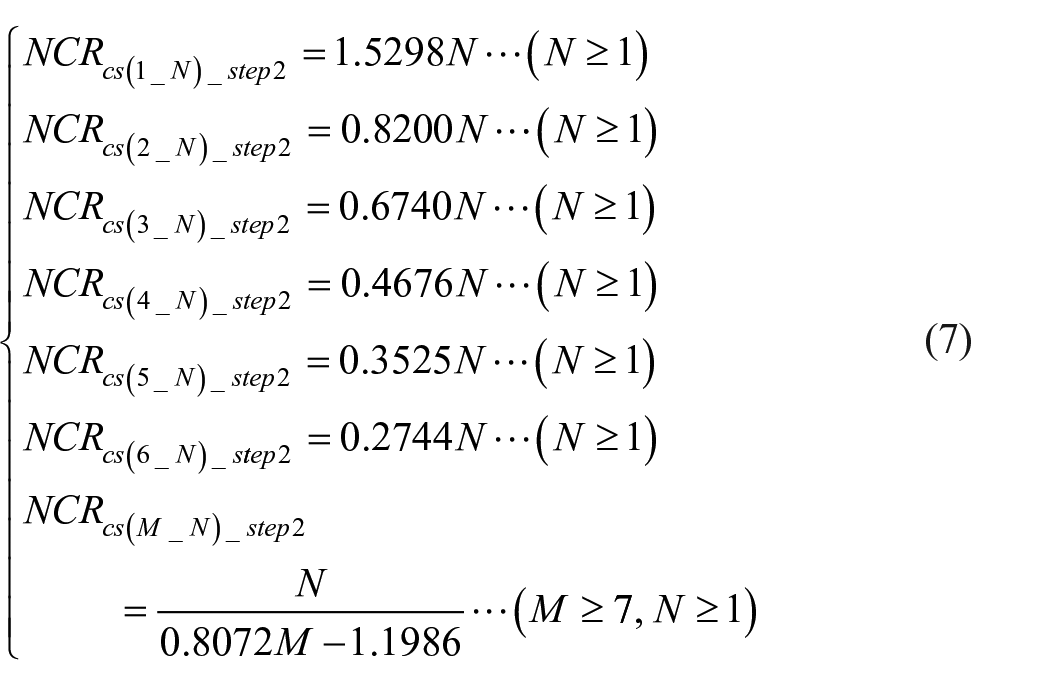
The calculations for the resistive network models in Initial State have been exhibited in Part 1,²³ and the relevant equations were summarized in Supplementary Model Calculation. Then, to inquire into the effect of models in different stages on the equivalent resistance, it is assumed that all contact resistances and length-related resistances have not changed with their values showed as equations (S51) in Supplemental Material. According to the resistive network models established in this article and using MATLAB software, the equivalent resistance expressions can be deduced, shown as equations (6) to (9), where equations (6) and (7) deliver the calculation results of the resistive network model involving RC₃, and equations (8) and (9) display the calculation results of the model ignoring RC₃.

{\begin{cases} N C R_{c s (1_N)_s t e p 1} = 1.9414 N - 0.4216 \dots (N \geq 1) \\ N C R_{c s (2_N)_s t e p 1} = 0.9707 N - 0.1507 \dots (N \geq 1) \\ N C R_{c s (3_N)_s t e p 1} = 0.4895 N + 0.1845 \dots (N \geq 1) \\ N C R_{c s (4_N)_s t e p 1} = 0.3305 N + 0.1370 \dots (N \geq 1) \\ N C R_{c s (5_N)_s t e p 1} = 0.2500 N + 0.1024 \dots (N \geq 1) \\ N C R_{c s (6_N)_s t e p 1} = 0.2011 N + 0.0732 \dots (N \geq 1) \\ N C R_{c s (M_N)_s t e p 1} = \frac{N}{0.9707 M - 0.8525} + \frac{1}{0.8072 M - 1.1986} - \frac{1}{0.9707 M - 0.8525} \dots (M \geq 7, N \geq 1) \end{cases}

(6)

{\begin{cases} N C R_{c s (1_N)_s t e p 2} = 1.5298 N \dots (N \geq 1) \\ N C R_{c s (2_N)_s t e p 2} = 0.8200 N \dots (N \geq 1) \\ N C R_{c s (3_N)_s t e p 2} = 0.6740 N \dots (N \geq 1) \\ N C R_{c s (4_N)_s t e p 2} = 0.4676 N \dots (N \geq 1) \\ N C R_{c s (5_N)_s t e p 2} = 0.3525 N \dots (N \geq 1) \\ N C R_{c s (6_N)_s t e p 2} = 0.2744 N \dots (N \geq 1) \\ N C R_{c s (M_N)_s t e p 2} = \frac{N}{0.8072 M - 1.1986} \dots (M \geq 7, N \geq 1) \end{cases}

(7)

{\begin{cases} C R_{c s (1_N)_s t e p 1} = 1.9414 N - 0.4216 \dots (N \geq 1) \\ C R_{c s (2_N)_s t e p 1} = 0.9707 N - 0.2108 \dots (N \geq 1) \\ C R_{c s (3_N)_s t e p 1} = 0.5014 N + 0.0750 \dots (N \geq 1) \\ C R_{c s (4_N)_s t e p 1} = 0.3380 N + 0.1263 \dots (N \geq 1) \\ C R_{c s (5_N)_s t e p 1} = 0.2549 N + 0.0864 \dots (N \geq 1) \\ C R_{c s (6_N)_s t e p 1} = 0.2046 N + 0.0652 \dots (N \geq 1) \\ C R_{c s (7_N)_s t e p 1} = 0.1709 N + 0.0508 \dots (N \geq 1) \\ C R_{c s (8_N)_s t e p 1} = 0.1467 N + 0.0415 \dots (N \geq 1) \\ C R_{c s (9_N)_s t e p 1} = 0.1285 N + 0.0349 \dots (N \geq 1) \\ C R_{c s (10_N)_s t e p 1} = 0.1144 N + 0.0300 \dots (N \geq 1) \\ C R_{c s (M_N)_s t e p 1} = \frac{N}{0.9643 M - 0.8984} + \frac{1}{0.8072 M - 1.1445} - \frac{1}{0.9643 M - 0.8984} \dots (M \geq 11, N \geq 1) \end{cases}

(8)

{\begin{cases} C R_{c s (1_N)_s t e p 2} = 1.5188 N \dots (N \geq 1) \\ C R_{c s (2_N)_s t e p 2} = 0.7599 N \dots (N \geq 1) \\ C R_{c s (3_N)_s t e p 2} = 0.5764 N \dots (N \geq 1) \\ C R_{c s (4_N)_s t e p 2} = 0.4642 N \dots (N \geq 1) \\ C R_{c s (5_N)_s t e p 2} = 0.3413 N \dots (N \geq 1) \\ C R_{c s (6_N)_s t e p 2} = 0.2698 N \dots (N \geq 1) \\ C R_{c s (7_N)_s t e p 2} = 0.2217 N \dots (N \geq 1) \\ C R_{c s (8_N)_s t e p 2} = 0.1882 N \dots (N \geq 1) \\ C R_{c s (9_N)_s t e p 2} = 0.1634 N \dots (N \geq 1) \\ C R_{c s (10_N)_s t e p 2} = 0.1444 N \dots (N \geq 1) \\ C R_{c s (M_N)_s t e p 2} = \frac{N}{0.8072 M - 1.1445} \dots (M \geq 11, N \geq 1) \end{cases}

(9)

Results and discussion

Changes of length-related and contact resistances in different tensile states

Assuming that the cross-sections of the conductive loops are all round with same size and the cross-sectional area is represented by A_s, then using the law of resistance,²⁴ the length resistance of each yarn segment can be determined by

{\begin{cases} R L_{1} = ρ \frac{L_{1}}{A_{s}}, R L_{1_1} = ρ \frac{L_{1_1}}{A_{s}}, R L_{1_2} = ρ \frac{L_{1_2}}{A_{s}} \\ R L_{2} = ρ \frac{L_{2}}{A_{s}}, R L_{2_1} = ρ \frac{L_{2_1}}{A_{s}}, R L_{2_2} = ρ \frac{L_{2_2}}{A_{s}} \\ R L_{3} = ρ \frac{L_{3}}{A_{s}} \end{cases}

(10)

Besides, according to Holm’s contact theory,²⁵

R_{C} = \frac{ρ}{2} \sqrt{\frac{π H}{n P}}

(11)

Among them, R_C means the contact resistance (Ω), ρ is the electrical resistivity (Ω/m), H indicates the material hardness (N/m²), n stands for the inner number of contact points within contact area, and P represents the contact pressure. Due to the values of ρ and H remaining unchanged when the environment and the material are determined, R_C is inversely proportional to n and P. Accordingly, each contact resistance can be calculated by

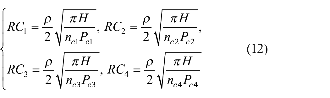
{\begin{cases} R C_{1} = \frac{ρ}{2} \sqrt{\frac{π H}{n_{c 1} P_{c 1}}}, R C_{2} = \frac{ρ}{2} \sqrt{\frac{π H}{n_{c 2} P_{c 2}}}, \\ R C_{3} = \frac{ρ}{2} \sqrt{\frac{π H}{n_{c 3} P_{c 3}}}, R C_{4} = \frac{ρ}{2} \sqrt{\frac{π H}{n_{c 4} P_{c 4}}} \end{cases}

(12)

The accurate values of the inner numbers of contact points (n_c₁, n_c₂, n_c₃, n_c₄) and contact pressures (P_c₁, P_c₂, P_c₃, P_c₄) are challenging to achieve. The changing trends of contact resistances can be analyzed instead by observing the variations of the loop in Supplemental Figure S12 and combining with equation (12).

By Supplementary Analysis of Changes in Length-related and Contact Resistances, the resistances’ changing trends in different tensile states can be summarized as Table 1, where “→” means the variable remains the same, “↗”and “↘” represent the rise and reduction of the variable, “↘↗” implies the variable goes down and then goes up, and “Inf” refers the variable is infinite.

Table 1.

The changing trends of length-related and contact resistances in different tensile states.

Resistances	From Initial State to Second State_1	From Second State_1 to Second State_2	From Second State_2 to Final State	During Final state
RL _{1_1}	→	→	↗	↗
RL _{1_2}	→	→	→	→
RL _{2_1}	→	→	→	→
RL _{2_2}	→	→	↗	↗
RL ₃	→	→	↘	↘↗
RC ₁	→	↗	↗	Inf
RC ₂	↗	Inf	Inf	Inf
RC ₃	↘	↘	↘	↘
RC ₄	→	↗	↗	↗

In practical applications, as the number of repetitive uses grows, the slippage and elongation of the yarn segment tend to cause irreversible deformation of the sensor, so controlling the strain range before these variations can improve the service life of the sensor. The introduction of elastic yarn in the plating stitch makes the fabric tighter so that the sensor can achieve the expected strain without the yarn slippage and elongation. As shown in Figure 6 and Table S1 in Supplemental Material, yarn slippage and elongation only occur if ε > 32%. The sensor can be used in the scenario needing the strain range in 0% to 32% due to its high repeatability and service life.

Mechanical–electrical performance analysis

The results of the mechanical–electrical property tests were depicted in Figure 7, containing the relationship curves of ΔR/R₀ and ε of the samples with different M(4, 10, 14) and N(50, 100, 150) and the relationship curves between the gauge factor G and ε, as displayed in Figure 7(a) and (b), respectively, where G can be determined by^12,20

G = \frac{Δ R / R_{0}}{ε}

(13)

It can be seen clearly from Figure 7 that the resistance change rate ΔR/R₀ increases non-linearly as the rise of ε. At the same time, G declines non-linearly as the rise of ε, and they both go up with the growth of N under fixing M and go down with the raise of M under fixing N.

Figure 7.

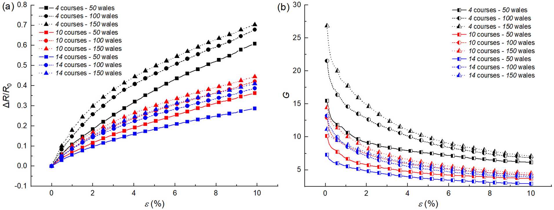
Results of the mechanical–electrical analysis: (a) curves of ΔR/R₀ and ε of the samples and (b) curves between the gauge factor G and ε.

Comparison the gauge factor G of experiment and model calculations

Assuming that the resistive network models are already close to those under Second State_1 when ε = 10%, that is, the equivalent resistance of the network can be calculated by those models in Second State, then the gauge factors can be determined by

{\begin{cases} N C G = \frac{(\begin{array}{l} N C R_{c s (M_N)_s t e p 1} \\ - N C R_{s t (M_N)} \end{array}) / N C R_{s t (M_N)}}{ε} \\ C G = \frac{(\begin{array}{l} C R_{c s (M_N)_s t e p 1} \\ - C R_{s t (M_N)} \end{array}) / C R_{s t (M_N)}}{ε} \end{cases}

(14)

Where NCG is the gauge factor calculated by the resistive network model with RC₃, while CG is the gauge factor calculated by the resistive network model without RC₃, and the remaining variables can be obtained from equations (6) and (8) and equations (S52) and (S53) in Supplemental Material.

Therefore, the gauge factor G, no matter in experiment or model calculations when ε = 10%, can be solved and the results corresponding to the prepared samples are listed in Table 2 and the expressions of NCG and CG corresponding to the sensor with different M and N (M>= 11, N ⩾ 1) can be achieved as

{\begin{cases} N C G = \frac{\begin{array}{l} 2.5385 * 10^{12} M + N (1.256 * 10^{12} M^{3} + 1.2226 * 10^{11} M^{2} - 5.2404 * 10^{12} M + 3.3995 * 10^{12}) + \\ 1.9636 * 10^{12} M^{2} - 3.6168 * 10^{11} M^{3} - 3.2412 * 10^{12} \end{array}}{\begin{array}{l} N (3.7183 * 10^{11} M^{3} - 1.1664 * 10^{12} M^{2} + 1.1647 * 10^{12} M - 3.7516 * 10^{11}) - \\ 4.272 * 10^{11} M - 6.7232 * 10^{10} M^{2} + 1.3693 * 10^{11} M^{3} + 3.3428 * 10^{11} \end{array}} \dots (M \geq 11) \\ C G = \frac{\begin{array}{l} 1.6524 * 10^{13} M + N (1.6432 * 10^{12} M^{3} + 5.0995 * 10^{12} M^{2} - 1.888 * 10^{13} M + 1.1835 * 10^{13}) - \\ 3.5851 * 10^{12} M^{2} + 1.3747 * 10^{11} M^{3} - 1.2393 * 10^{13} \end{array}}{\begin{array}{l} N (7.5059 * 10^{11} M^{3} - 2.4628 * 10^{12} M^{2} + 2.6343 * 10^{12} M - 9.2365 * 10^{11}) - \\ 1.8879 * 10^{12} M + 5.0985 * 10^{11} M^{2} + 1.6432 * 10^{11} M^{3} + 1.1835 * 10^{12} \end{array}} \dots (M \geq 11) \end{cases}

(15)

Table 2.

When ε = 10%, the gauge factor G of the experiment and model calculations.

M–N	G (the gauge factor)
	Experiment							NCG	CG
	1	2	3	4	5	Mean	SD	NCG	CG
4–50	6.1241	6.1347	6.1448	6.1309	6.1387	6.1345	0.0078	6.8203	6.6498
4–100	6.8321	6.8441	6.8481	6.8412	6.8477	6.8414	0.0066	6.8625	6.6992
4–150	7.0729	7.0785	7.0812	7.0731	7.0793	7.0775	0.0038	6.8768	6.7158
10–50	3.6471	3.6601	3.6658	3.6542	3.6628	3.6577	0.0074	4.5220	3.7055
10–100	4.2473	4.2564	4.2395	4.2455	4.2593	4.2478	0.0081	4.5487	3.7204
10–150	4.4729	4.4896	4.4850	4.4775	4.4827	4.4825	0.0065	4.5577	3.7255
14–50	2.8701	2.8932	2.9104	2.8758	2.9001	2.8912	0.0168	4.1596	3.2364
14–100	3.8980	3.9234	3.8894	3.9013	3.9171	3.9036	0.0140	4.1847	3.2473
14–150	4.1192	4.1449	4.1096	4.1172	4.1445	4.1246	0.0165	4.1935	3.2512

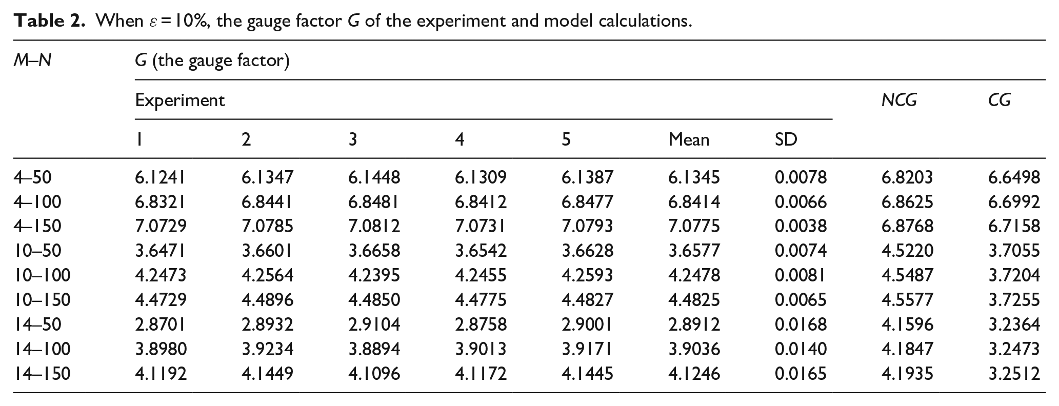
It can be gotten that there exist specific gaps between the experimental and model calculation data by plotting the data in Table 2, resulting in Figure 8. Moreover, their data changing trends are consistent, that is, each kind of G goes down with the rise of M under fixing N (see Figure 8(a)–(c)) and goes up with the raise of N under fixing M (see Figure 8(d)–(f)). It should be noted that when M is fixed, the increasing trend of G of the experiment is evident. Simultaneously, the model calculations, NCG and CG, are not apparent with the increase of N, which is related to the loops’ geometrical regularity and the relative spatial position of the face and ground yarns in the real samples. In contrast, the loop corresponding to the resistive network model is assumed to be an ideal state. In addition, the NCG of each sensor specification is higher than CG. The calculating G of the resistive network model with RC₃ is higher than that of the network model without RC₃, indicating the presence of the interlocking contact resistance RC₃ can improve the sensor’s gauge factor.

Figure 8.

When ε = 10%, the comparison of the gauge factor G of the experiment and model calculations: (a–c) fixing the wale number N (50, 100, 150) separately, the plots of G and course number M and (d–f) fixing the course number M (4, 10, 14) separately, the plots of G and wale number N.

Next, MATLAB was used to make the three-dimensional surface graphs of equation (15) illustrated in Figure 9. Figure 9(a) is a comprehensive three-dimensional surface graph of NCG and CG, clearly indicates that NCG is always higher than CG. From the respective three-dimensional surface plots of NCG and CG in Figure 9(b) to (e), it can be achieved that NCG and CG both ascend with the rise of N in a decreasing rate and descend with the growth of M in a reducing rate. Then, NCG and CG both finally tend to be a stable value with the raises of M and N. It can be suggested that the effect of M on the gauge factor is greater than that of N on gauge factor from the projections on the x–y plane combined with the color bars. Therefore, in the case of the determination of raw materials and applying the voltage on the ends of course, in order to design a sensor with high sensitivity, the primary method is to determine the number of conductive courses as low as possible, followed by increasing the number of conductive wales.

Figure 9.

When ε = 10%, the relationships among NCG, CG, M, and N: (a) 3-D surface of NCG and CG in the same coordinate, (b and c) relationship among NCG, M, and N, and (d and e) relationship among CG, M, and N.

Effect of contact resistances on equivalent resistance during the stretching form Initial State to Second State_1

As displayed in Table 1 and Supplemental Figure S12, during the stretching form Initial State to Second State_1, each length-related resistance remains unchanged and the most significant change is that RC₂ increases, RC₃ decreases while RC₁ and RC₄ are unchanged. In addition, the resistances’ connections in the resistive network model are the same as those established in Part 1²³ until the RC₂ disappear in the model. So, the resistive network model in Part 1 is induced to discuss the effects of RC₂ and RC₃ on the equivalent resistance during the stretching form Initial State to Second State_1.

The graphs of NCR_st _{(M_N)} with RC₂ and RC₃ can be made by MATLAB, as shown in Figure 10, through using the initial value of each resistance except for RC₂ and RC₃ in equation (S51) in Supplemental Material, where RC₂ takes the value range of 3.0230 to 2500 and RC₃ is from 0 to 0.3528. Figure 10(a) to (f) show the respective graph when M is fixed at 4, 10, and 14 separately. Figure 10(g) to (l) depict the individual graph when N is fixed at 50, 100, and 150 respectively. They indicate that NCR_st _{(M_N)} increases to a specific value with the rise of RC₂, declines negligibly with the growth of RC₃, and ascends as N rises and reduces as M raises.

Figure 10.

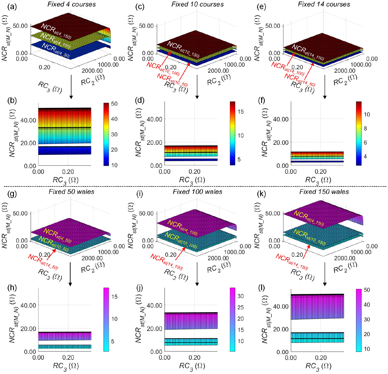
Impacts of RC₂ and RC₃ on NCR_st _{(M_N)} form Initial State to Second State_1: (a–f) fixing course number M separately, the 3-D surfaces of NCR_st _{(M_N)}, RC₂ and RC₃ and their projections on RC₃-NCR_st _{(M_N)} plane and (g–l) fixing wale number N separately, the 3-D surfaces of NCR_st _{(M_N)}, RC₂ and RC₃ and their projections on RC₃-NCR_st _{(M_N)} plane.

In the same way, the relationship between CR_st _{(M_N)} and RC₂ is explored using the resistive network model without RC₃ in Part 1.²³ As shown in Figure 11, CR_st _{(M_N)} goes up as RC₂ rises and tends to a stable value, and grows with the increase of N and decreases with the raise of M.

Figure 11.

Impact of RC₂ on CR_st _{(M_N)} form Initial State to Second State_1.

Effect of different tensile states on equivalent resistance

According to equation (S52) in Supplemental Material and equations (6) and (7), the analysis results of the equivalent resistance of the sensor with different M and N at different stretching stages can be conducted in Figures 12 and 13. It can be gotten that NCR_st _{(M_N)} < NCR_cs _{(M_N)_step1} < NCR_cs _{(M_N)_step2} except for M = 1, 2 (NCR_st _{(M_N)} < NCR_cs _{(M_N)_step2} < NCR_cs _{(M_N)_step1}), and each of them decreases non-linearly as M grows and increases linearly as N rises. Also, the differences among the resistances in different tensile states ascend with the growth of N and descend with the raise of M.

Figure 12.

Fixing course number M, the plots of resistance and wale number N of different models concerning RC₃, where 1 = <M, N< = 10: (a) when N = 1, 2, 3, 4, 5 and (b) when N = 6, 7, 8, 9, 10.

Figure 13.

When M> = 11 and N> = 1, the 3-D surface of the resistance, M and N of the diverse models concerning RC₃ and their projections on each plane: (a) 3-D surface, (b) projection on the x–z plane, and (c) projection on the y–z plane.

Meanwhile, equation (S53) in Supplemental Material and equations (8) and (9) are analyzed, resulting in Figures 14 and 15. Similarly, it can be implied that CR_st _{(M_N)} < CR_cs _{(M_N)_step1} < CR_cs _{(M_N)_step2} except for M = 1, 2 (CR_st _{(M_N)} < CR_cs _{(M_N)_step2} < CR_cs _{(M_N)_step1}), each of them reduces non-linearly as M increases and grows linearly as N rises. The differences among them goes up as N ascends and goes down as M raises.

Figure 14.

Fixing course number M, the plots of resistance and wale number N of different models without concerning RC₃, where 1 = <M, N< = 10: (a) when N = 1, 2, 3, 4, 5 and (b) when N = 6, 7, 8, 9, 10.

Figure 15.

When M> = 11 and N> = 1, the 3-D surface of the resistance, M and N of the diverse models without concerning RC₃ and their projections on each plane: (a) 3-D surface, (b) projection on the x–z plane, and (c) projection on the y–z plane.

Here, the reason of NCR_cs _{(M_N)_step2} < NCR_cs _{(M_N)_step1} and CR_cs _{(M_N)_step2} < CR_cs _{(M_N)_step1} when M = 1, 2 is that the variations of the related resistances during the elongation has not been taken into account, just using the same values of the resistances as those in Initial State.

Conclusion

This article has further established and calculated the resistive network model of the weft-knitted strain sensor with the plating stitch during the elongation along course direction. It can be seen that the resistive network model of the sensor changes with the conductive loops’ configuration and contact situation. Similar to the method for establishing model in Part 1 of this series,²³ two models with one including RC₃ and the other not were explored. In the case of applying the voltage at two ends of the course, the resistive network at different elongation stages was simplified to a series-parallel resistive network which is connected in series along course direction and parallel along the wale direction. It can be verified from experiment and theoretical analysis that the sensor’s equivalent resistance, under a specific elongation, increases linearly with the rise of conductive wale number and decreases non-linearly with the rise of conductive course number.

Through experiment and model calculation, it can be obtained that in the initial stage of stretching, the contact resistances’ changes are the main factors affecting the mechanical–electrical performance of the sensor. Then as the sensor is further stretched, the length-related resistances of the conductive yarn segments begin to affect the sensor’s mechanical–electrical properties due to yarns’ slippage and self-elongation. In addition, the weft jacquard plating technology makes the strain of the sensor reach about 32% before yarns’ slippage and self-elongation, which expands the sensor’s measurable strain range, and avoids irreversible deformation of the sensor after repeated use in this range. According to the results and discussion, the sensor with high gauge factor can be obtained by reducing the number of conductive courses and increasing the number of wales in the sensing area. At the same time, the ground yarn’s diameter should be lower than that of the conductive face yarn to avoid reducing the gauge factor during stretching.

Admittedly, because it is challenging to determine the values of the diverse concerning resistances in the resistive network under all tensile state from the experiment, the experimental section in this article mainly focused on the elongation from Initial State to Second State_1.

The research in this article will help the subsequent design and preparation of suitable sensors for monitoring limb movements, such as hand movements, elbow joint movements, and knee joint movements.

Supplemental Material

Supplementary_Materials – Supplemental material for Resistive network model of the weft-knitted strain sensor with the plating stitch-Part 2: Resistive network model during the elongation along course direction

Supplemental material, Supplementary_Materials for Resistive network model of the weft-knitted strain sensor with the plating stitch-Part 2: Resistive network model during the elongation along course direction by Yujing Zhang and Hairu Long in Journal of Engineered Fibers and Fabrics

Footnotes

Declaration of conflicting interests

The author(s) declared no potential conflicts of interest with respect to the research, authorship, and/or publication of this article.

Funding

The author(s) received no financial support for the research, authorship, and/or publication of this article.

ORCID iD

Yujing Zhang

Supplemental material

Supplemental material for this article is available online.

References

Miao

Niu

, et al. Human motion recognition of knitted flexible sensor in walking cycle. Sensors 2020; 20(35): 1–14.

Wang

Soltanian

Servati

, et al. A knitted wearable flexible sensor for monitoring breathing condition. J Eng Fibers Fabr 2020; 15: 1–13.

Tian

, et al. Multiscale disordered porous fibers for self-sensing and self-cooling integrated smart sportswear. Acs Nano 2020; 14: 559–567.

Miao

Raji

RK.

Flexible knitted sensing device for identifying knee joint motion patterns. Smart Mater Struct 2019; 28(11): 1–9.

Han

Miao

Chen

, et al. Research on finger movement sensing performance of conductive gloves. J Eng Fibers Fabr 2019; 14: 1–7.

Raji

Miao

Wan

, et al. Knitted piezoresistive smart chest band and its application for respiration patterns assessment. J Eng Fibers Fabr 2019; 14(4): 1–14.

Atalay

Kennon

Demirok

Weft-knitted strain sensor for monitoring respiratory rate and its electro-mechanical modeling. IEEE Sens J 2015; 15: 110–122.

Raji

Miao

Zhang

, et al. Knitted piezoresistive strain sensor performance, impact of conductive area and profile design. J Ind Text 2020; 50(5): 616–634.

Liu

The impact of different proportions of knitting elements on the resistive properties of conductive fabrics. Text Res J 2019; 89: 881–890.

10.

Tohidi

Zille

Catarino

, et al. Effects of base fabric parameters on the electro-mechanical behavior of piezoresistive knitted sensors. IEEE Sens J 2018; 18: 4529–4535.

11.

Raji

Miao

Zhang

, et al. Influence of rib structure and elastic yarn type variations on textile piezoresistive strain sensor characteristics. Fibres Text East Eur 2018; 26: 24–31.

12.

Atalay

Tuncay

Husain

, et al. Comparative study of the weft-knitted strain sensors. J Ind Text 2017; 46: 1212–1240.

13.

Xie

Long

HR.

Investigation on the relation between structure parameters and sensing properties of knitted strain sensor under strip biaxial elongation. J Eng Fibers Fabr 2015; 10: 166–178.

14.

Atalay

Kennon

Husain

MD.

Textile-based weft knitted strain sensors: effect of fabric parameters on sensor properties. Sensors 2013; 13: 11114–11127.

15.

Zhang

Relationship between mechanical-electrical properties and fabric structures made from intrinsically conductive fibers. In: Tao

(ed.) Handbook of smart textiles. Singapore: Springer, 2015, pp.719–737.

16.

Zhang

Tao

Wang

, et al. Electro-mechanical properties of knitted fabric made from conductive multi-filament yarn under unidirectional extension. Text Res J 2005; 75: 598–606.

17.

Liu

Ding

, et al. Electromechanical analysis of length-related resistance and contact resistance of conductive knitted fabrics. Text Res J 2012; 82: 2062–2070.

18.

Wan

, et al. A resistive network model for conductive knitting stitches. Text Res J 2010; 80: 935–947.

19.

Wang

Long

Soltanian

, et al. Electromechanical properties of knitted wearable sensors: part I - theory. Text Res J 2014; 84: 3–15.

20.

Wang

Long

Soltanian

, et al. Electro-mechanical properties of knitted wearable sensors: part 2-parametric study and experimental verification. Text Res J 2014; 84: 200–213.

21.

Xie

Long

HR.

Equivalent resistance calculation of knitting sensor under strip biaxial elongation. Sens Actuator A-phys 2014; 220: 118–125.

22.

Wang

Long

HR.

Research on wearable sensors based on knitted fabrics with silver plating fiber. Adv Mater Resswitz 2011; 331: 36–39.

23.

Zhang

Long

HR.

Resistive network model of the weft-knitted strain sensor with the plating stitch-part 1: resistive network model under static relaxation. J Eng Fibers Fabr 2020; 15: 1–16.

24.

Alexander

Sadiku

MNO

. Part1: DC circuits fundamentals of electric circuits. 6th ed. New York: McGraw-Hill Education, 2017, pp.3–77.

25.

Holm

Electric contacts: theory and application. 4th ed. New York: Springer Science & Business Media, 1967.

Supplementary Material

Please find the following supplemental material available below.

For Open Access articles published under a Creative Commons License, all supplemental material carries the same license as the article it is associated with.

For non-Open Access articles published, all supplemental material carries a non-exclusive license, and permission requests for re-use of supplemental material or any part of supplemental material shall be sent directly to the copyright owner as specified in the copyright notice associated with the article.

0.00 MB

11.20 MB

Resistive network model of the weft-knitted strain sensor with the plating stitch-Part 2: Resistive network model during the elongation along course direction

Abstract

Keywords

Introduction

Loop configurations and resistance distributions under deformation

Establishment and calculation of the resistive network models under deformation

Resistive network model containing RC3

Resistive network model ignoring RC3

Experiment and model calculation

Materials prepared

Measurements of the strain along course direction in different tensile states

Mechanical–electrical performance testing

Calculations of resistive network models in different tensile states

Results and discussion

Changes of length-related and contact resistances in different tensile states

Mechanical–electrical performance analysis

Comparison the gauge factor G of experiment and model calculations

Effect of contact resistances on equivalent resistance during the stretching form Initial State to Second State_1

Effect of different tensile states on equivalent resistance

Conclusion

Supplemental Material

Supplementary_Materials – Supplemental material for Resistive network model of the weft-knitted strain sensor with the plating stitch-Part 2: Resistive network model during the elongation along course direction

Footnotes

Declaration of conflicting interests

Funding

ORCID iD

Supplemental material

References

Supplementary Material

Resistive network model containing RC₃

Resistive network model ignoring RC₃