Sage Journals: Discover world-class research

Abstract

The resistive network model of the weft-knitted strain sensor with the plating stitch under static relaxation is studied based on the knitted loop structure and circuit principle. The prepared sensors are divided into the sensing area and the non-sensing area. The former consists of the conductive face yarn and the insulated elastic ground yarn, while the latter includes the normal face yarn and the same ground yarn. The loop of conductive face yarn not only produces length-related resistance but also causes the jamming contact resistances along the width and length direction. Besides, the elastic ground yarn has a potential impact on the contact situation of the conductive face yarn at the interlocking point, determining whether the interlocking contact resistance exists. Therefore, two resistive network models have been established accordingly. In addition to the length-related resistance, the first model focused on both the jamming and interlocking contact resistances, while the second one only dealt with the jamming contact resistance. In the case of applying voltage along the two ends of the course, the theoretical calculations of the corresponding network models were performed using a series of equivalent transformations. Finally, the correctness and usability of the two models were verified through experiments and model calculations. It was found that both models can predict that the equivalent resistance increases with the conductive wale number and decreases with the conductive course number. It was implied that the first model’s calculating resistances are closer to the experimental data and lower than those of the second model. The difference in the calculating resistances of the two models would become smaller as the course number increases. Thus, the investigation indicates that the jamming contact resistance has a more considerable influence on the resistive network than the interlocking contact resistance.

Keywords

Resistive network model weft-knitted strain sensor plating stitch jamming contact resistance interlocking contact resistance length-related resistance

Introduction

Knitted strain sensors, owing to their excellent extensibility and elastic recovery, have been increasingly used in body motion sensing and physiological parameter monitoring in recent years,^1–11 such as elbow and knee movement monitoring,^1,2,5,9,11 hand movement monitoring,^2,5,8,10,11 and respiratory monitoring.^2,6,7 There remain various methods used to prepare the knitted strain sensors in which applying conductive yarns to knitted strain sensors directly through knitting technology is the preferred method for some researchers.^1,2,6–9 Besides, there exist investigators using knitted fabric as substrates to make conductive strain sensors by chemical treatment.^10,11 Also, sewing the conductive yarn or conductive thread on high-elastic knitted fabric can get the strain sensors.⁵ The new worm-shaped filaments,³ with distinctive strain-insensitive behavior, provide a choice for the connection between knitted strain sensor and data acquisition unit.

The knitted strain sensors can be adopted if they have high sensitivity and repeatability, which is determined by their internal circuits. Therefore, some scholars have studied their internal resistive network model and analyzed their mechanical-electrical properties in tension verified by experiments. Zhang¹² and Zhang et al.¹³ studied the mechanical-electrical performance of weft jersey strain sensors from the fiber-yarn-fabric levels. Furthermore, they gave a general method for calculating the equivalent resistance of the resistive network. Li et al.^14–16 established a resistive network for weft plain strain sensors and experimentally investigated the effects of length-related resistance and contact resistance on the mechanical-electrical properties of the sensors in unidirectional tension. Wang et al.^17,18 further improved the solution of the resistive network and mechanical-electrical analysis of the weft-knitted sensors based on the resistive network model given by Zhang et al.¹³ Further, they explored the factors affecting the sensor performance in combination with experiments. Xie and Long^19,20 solved the resistive network model of weft-knitted strain sensors under biaxial elongation and analyzed the corresponding mechanical-electrical properties. Liu et al.^21,22 further enriched the influences of float and tuck stitches on the resistive network of weft-knitted strain sensors. These mechanism studies have generally concluded that the knitted strain sensors’ mechanical-electrical properties are related to the resistive network composed of the length-related resistance of the conductive yarn loops and the contact resistance due to the touching of the loops. It is universally acknowledged that the length-related resistance is concerned with the diameter and electrical conductivity of the conductive yarn, and the contact resistance is related to the hardness, resistivity, contact area, and pressure of the conductive material itself. The connection between various resistors in the resistive network depends on the stitch of the knitted strain sensors and the contact situation between the conductive yarns. Furthermore, above all, the way of the voltage loaded on the sensors affects the final equivalent resistance.

It has been proven that the sensitivity, repeatability, and stability of the knitted strain sensor can be effectively improved through the weft plating technology, that is, using the conductive yarn as the face yarn and the insulated elastic yarn as the ground yarn in the sensing area.^19,23,24 The addition of an elastic ground yarn increases the contact between conductive yarn loops, thereby changing the type and distribution of internal contact resistances. However, the existing resistive network models rarely take various contact resistances into account, usually only considering the contact resistance caused by the interlocking of the conductive yarn loops while ignoring those caused by the jamming of the loops. Furthermore, these different types of contact resistances and the length-related resistances separated by the contact points in the resistive model are dynamically changing to respond to strain when the sensor is extended. Thoroughly studying the effects of these contact resistances and length-related resistance can more clearly understand the sensing mechanism of knitted strain sensors, and provide theoretical support in sensor optimization. Hong et al.²⁵ established a resistive network model regarding the jamming and interlocking contact resistances of a compact knitted strain sensor. However, this model aimed at a weft jersey strain sensor in a circular form with the voltage is applied at both ends in the wale direction.

This article takes the weft-knitted strain sensor with the plating stitch as the research object and focuses on studying its internal resistive network under static relaxation to modify the existing models. The effects of the elastic ground yarn on the resistive network will be thoroughly examined, including the re-divided length-related resistance, the jamming contact resistance, and the interlocking contact resistance. In the case of applying voltage along the two ends of the course, the two internal resistive networks are modeled, and their equivalent resistances are calculated. Finally, the newly established models are used to calculate the equivalent resistance of the resistive network with specific numbers of conductive loop course and wale to further verify the correctness and usability of the model by comparing it with the experimental data.

The basic unit of the weft-knitted strain sensor with the plating stitch

Weft jacquard plating technology

Based on the weft jacquard plating technology, three kinds of yarn were used to prepare the knitted strain sensor, including the sensing area and non-sensing area (see Figure 1). As shown in Figure 1(a)–(b), the conductive yarn (colored with black) and the insulated elastic yarn (colored with white) are used as the face yarn and the ground yarn in the sensing area, respectively. The normal yarn (colored with gray) used as the face yarn and the same ground yarn consists of the non-sensing area.

Figure 1.

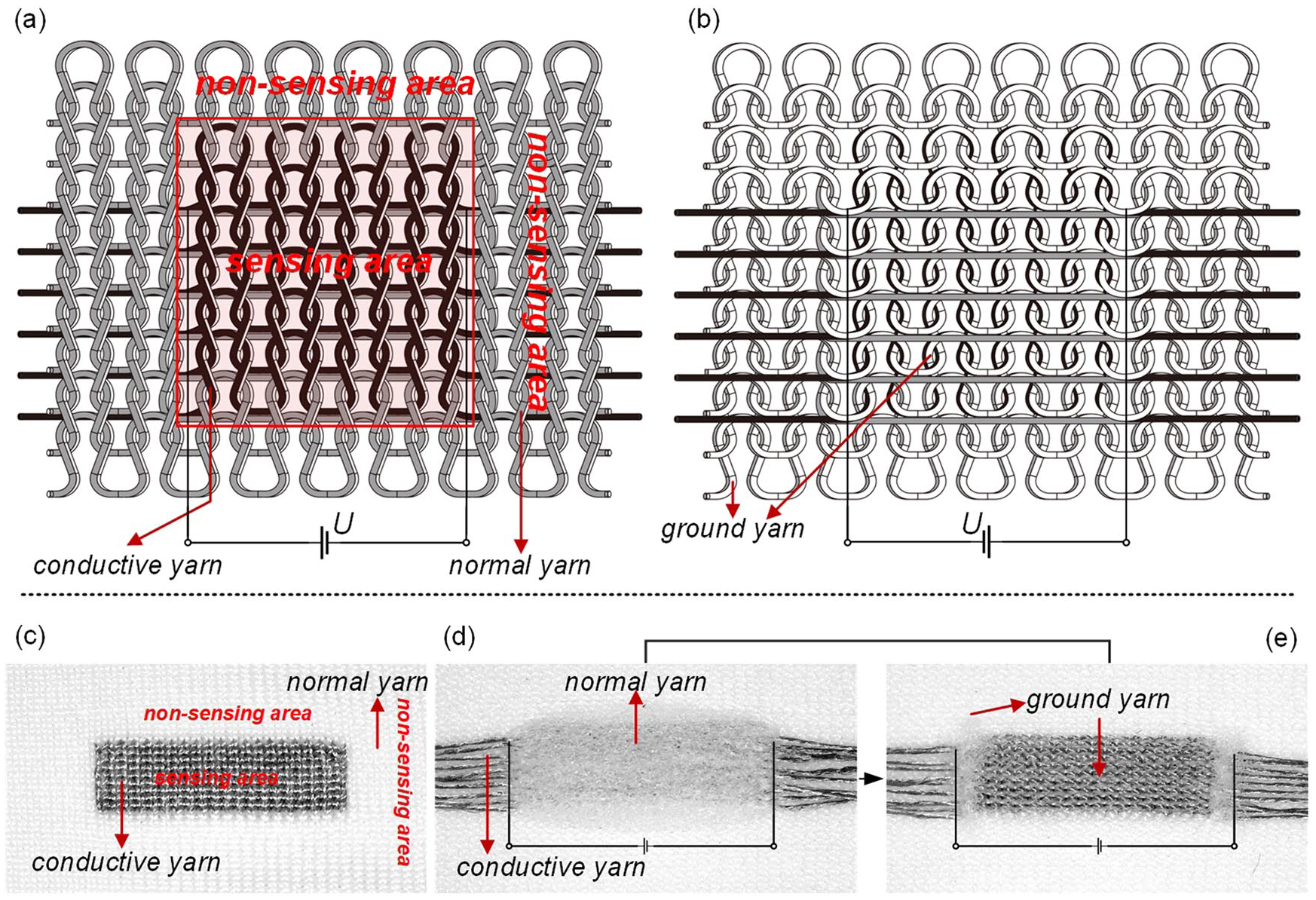
Schematic and physical diagrams of weft-knitted strain sensor prepared by the weft jacquard plating technology: (a, b) Schematic diagrams of the strain sensor, including (a) Front Side and (b) Reverse Side, being composed of sensing area and non-sensing area, and (c–e) the corresponding physical diagrams of the strain sensor, containing (c) Front Side and (d, e) Reverse Side.

Figure 1(c)–(e) displays the real knitted strain sensor. Herein, the conductive yarn in the sensing area is silver-plated nylon filament. In contrast, the face yarn in the non-sensing area is low-elastic nylon filament, and the ground yarns of both areas are nylon/spandex covered yarn. Besides, the floats of normal yarns (see Figure 1(d)) in the reverse side of the sensing area were cut off (see Figure 1(e)) in order not to interfere with the stretch and recovery of the sensor. Besides, the voltage is loaded on the conductive floats along the two ends of the loop courses.

The definitions of the concerning contact resistances

The weft plating technology makes the plating fabric (shown in Figure 2(c)–(d)) tighter and more uniform than the plain fabric, as displayed in Figure 2(a)–(b), due to the addition of elastic ground yarn. The plain fabric only has the interlocking contacts between conductive yarns (Figure 2(a)–(b)). In contrast, the plating fabric shows the jamming contacts between conductive yarns both along the width and length direction (Figure 2(c)–(d)). Thus, the corresponding contact resistances are defined as RC₁, RC₂, RC₄, and RC₃, respectively; among them, RC₁ and RC₂ represent the jamming contact resistances along the width direction, RC₄ is the jamming contact resistance along the length direction, and RC₃ indicates the interlocking contact resistance. As illustrated in the enlarged views in Figure 2(c)–(d), the ground yarn isolates the contacts between conductive yarns of the interlocking points, which causes the disappearance of RC₃. Therefore, two resistive network models are established in this article. The first model deals with both the jamming and interlocking contact resistances, and the second one only focuses on the jamming contact resistances.

Figure 2.

Comparison of physical diagrams of the weft-knitted strain sensor without and with the plating stitch separately and definitions of the concerning contact resistances: (a, b) Physical diagrams of the strain sensor without the plating stitch, including (a) Front Side and (b) Reverse Side (b), with the enlarged views of interlocking points with RC₃, and (c, d) physical diagrams of the strain sensor with the plating stitch marked with RC₁, RC₂, and RC₄, containing (c) Front Side and (d) Reverse Side, with the enlarged views of interlocking points without RC₃.

Establishment and theoretical calculation of the resistive network models under static relaxation

In this section, the following models are therefore discussed separately:

Resistive network model with RC₁, RC₂, RC₃, and RC₄;

Resistive network model with RC₁, RC₂, and RC₄;

From now on, it should be noted that M and N mean the number of loop courses and wale in the sensing area, respectively.

Resistive network model with RC₁,RC₂,RC₃, and RC₄

After specifying the various contact resistances, the length-related resistances re-divided by the jamming and interlocking contacts between conductive yarn loops should be defined. Peirce’s geometrical model of the plain stitch is used to observe the distribution of the different resistors (see Figure 3).²⁶ The actual contact area is minimal due to the current constriction at the contact points,^17,27 so the contact areas are simplified to small points dividing the conductive yarns to some length sections. In Figure 3(a) and (c), L₁ represents the total length of the needle loop, L_{1_1} and L_{1_2} are the partial lengths of the needle loop divided by the points of RC₁ and RC₄, L₂ indicates the total length of the sinker loop, L_{2_1} and L_{2_2} are the partial lengths of the sinker loop divided by the points of RC₂ and RC₄, and L₃ refers to the length of the leg, respectively. Therefore, the corresponding length-related resistances are defined as RL₁, RL_{1_1}, RL_{1_2}, RL₂, RL_{2_1}, RL_{2_2}, and RL₃. Besides, assuming L as the total loop length, its corresponding length-related resistance is expressed as RL. Then, according to the geometry model, the relationships of these length-related resistances can be described as

{\begin{cases} R L = R L_{1} + R L_{2} + 2 R L_{3} \\ R L_{1} = R L_{1_1} + 2 R L_{1_2} \\ R L_{2} = 2 (R L_{2_1} + R L_{2_2}) \end{cases}

(1)

Figure 3.

Distributions and definitions of the contact resistances and length-related resistances, using Peirce’s ²⁶ geometrical model of the plain stitch: (a) Front Side marked with resistances, (b) Cross-Section corresponded with (a), and (c) Reverse Side corresponded with (a).

Hence, referring to the distribution of diverse resistances in the geometrical models (see Figures 4(a) and (c) and 5(a) and (c)), the prototypical resistive networks of the weft-knitted sensor with different M and N can be constructed as shown in Figures 4(b) and (d) and 5(b) and (d). It can be concluded as the following:

When M ⩾ 1, the resistive networks all contain RC₁ and RC₂ when N ⩾ 2 and only contain RC₂ when N = 1;

When M ⩾ 2, RC₃ occurs in the network due to the interlocking between conductive yarns;

When M ⩾ 3, RC₄ appears in the network because of the contact between the courses separated by one course.

During the theoretical calculations of the resistive network models, some equivalent transformations are used to simplify the model to the easy-to-solve resistive network. The existing theoretical models have been confirmed that the equivalent resistances of the knitted plain strain sensors are proportional to the wale number when the voltage is applied to both ends of the course direction.^16,17,22

Figure 4.

Distributions of diverse resistances and prototypical resistive network model concerning RC₃: (a) Distribution of diverse resistances in the geometrical model when M = 1, (b) prototypical resistive network when M = 1, (c) distribution of diverse resistances in the geometrical model when M = 2, and (d) prototypical resistive network when M = 2.

Figure 5.

Distributions of diverse resistances and prototypical resistive network model concerning RC₃: (a) Distribution of diverse resistances in the geometrical model when M = 3, (b) prototypical resistive network when M = 3, (c) distribution of diverse resistances in the geometrical model when M ⩾ 4, and (d) prototypical resistive network when M ⩾ 4.

Therefore, in this article, under applying the voltage to both ends of the course direction, the resistance network model can be rearranged based on the distribution of conductive loops along the course direction. As embodied in Figure 6, after exchanging the two semi-wales named P₁ and P₂ in Figure 6(a), a new simplified sensor structure illustrated in Figure 6(b) is obtained. The two semi-wales at the course ends are combined to form a conductive wale without RC₁ (referred to as the N-RC₁-wale, Figure 6(c)), and the rest part of the sensor is repeated N − 1 times by another conductive wale with RC₁ (referred to as the RC₁-wale, Figure 6(d)) along the course direction. Therefore, the rearranged sensor’s voltage distribution conforms to equation (2), where U₁ and U₂ are applied to the N-RC₁-wale and RC₁-wale, respectively

U = U_{1} + (N - 1) \times U_{2}

(2)

According to Ohm’s law,²⁸ the relationship between the total resistance and each series resistance can be deduced as

\begin{array}{l} N C R_{s t (M_N)} = N C R_{s t (M_1)} \\ + (N - 1) \times N C R_{s t t (M_1)} \dots (M \geq 1, N \geq 1) \end{array}

(3)

where NCR_st _{(M_N)} represents the total equivalent resistance of the sensor with M courses and N wales, NCR_st _{(M_1)} indicates the equivalent resistance of the sensor with M courses and one wale which refers to the N-RC₁-wale, and NCR_stt _{(M_1)} is the equivalent resistance of the sensor’s repeat area which refers to the RC₁-wale.

Figure 6.

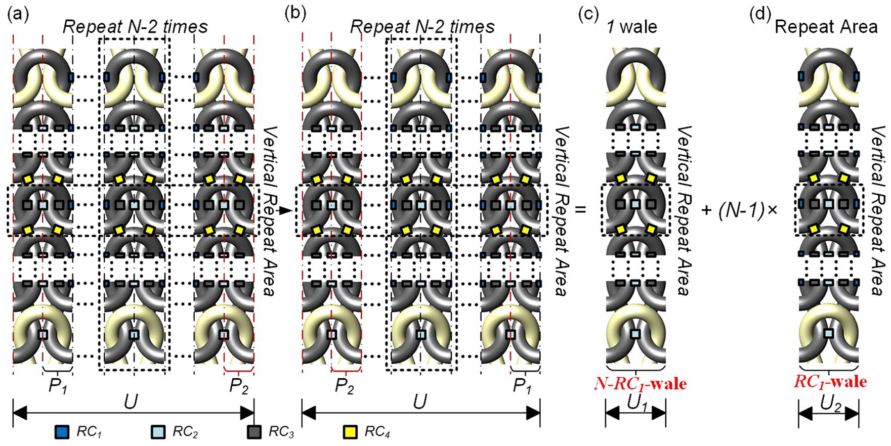
Simplifying the weft-knitted sensor’s geometrical model when voltage is applied to both ends of the course direction: (a) The initial structure marked with resistances, (b) the final structure after exchanging P₁ and P₂ in (a), (c) the N-RC₁-wale composed of the two semi-wales at the course ends in (a), and (d) the RC₁-wale meaning the repeat area along the course direction in (a).

By Supplementary Theoretical Calculation 1, the final equivalent resistive circuits of NCR_st _{(M_1)} and NCR_stt _{(M_1)} with different M and their corresponding equations can be summarized in Figure 7, where the symbol “//” indicates the parallel of resistances. During the calculation, a series of equivalent transformations (Supplemental Figures S1–S6), such as evenly dividing the contact resistors into the branches connected to themselves,^16,21,22 splitting the nodes on the symmetry line, the merge of equipotential points, the Y − Δ transformations,²⁸ the nodal analysis,²⁸ the series-parallel rule of resistance,²⁸ and removing the bridge resistors in the generalized Wheatstone bridge,¹⁶ were used. So far, the theoretical calculation of NCR_st _{(M_N)} with different M and N can be summarized as shown in equation S20 in Supplemental Material.

Figure 7.

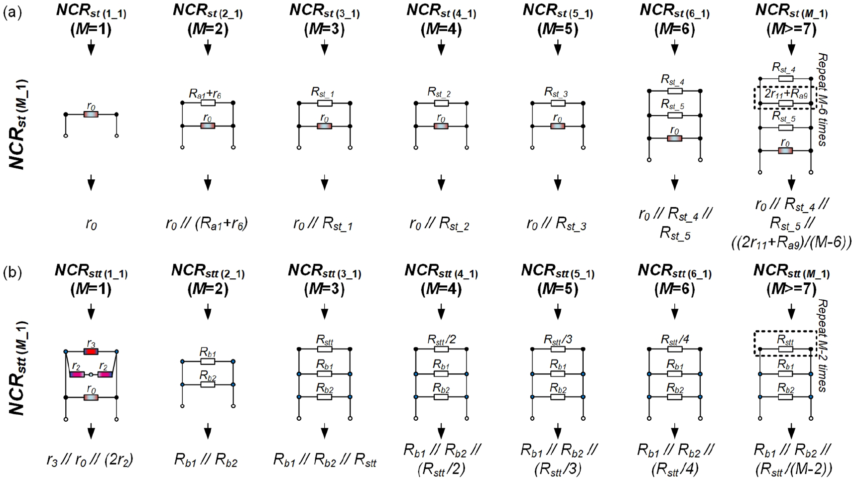
Final equivalent resistive circuits of NCR_st _{(M_1)} and NCR_stt _{(M_1)} with different M and their corresponding formulas: (a) Circuits and formulas of NCR_st _{(M_1)} with different M and (b) circuits and formulas of NCR_stt _{(M_1)} with different M.

Resistive network model with RC₁, RC₂, and RC₄

The resistive network model with RC₁, RC₂, and RC₄ is only considering the jamming contact resistance. Here, the total equivalent resistance of the sensing area with M courses and N wales is named as CR_st _{(M_N)}, and the equivalent resistances of N-RC₁-wale and RC₁-wale are labeled as CR_st _{(M_1)} and CR_stt _{(M_1)}, respectively. Then, as shown in Figure 6, the relationship between the total resistance and each series resistance can be described as

\begin{array}{l} C R_{s t (M_N)} = C R_{s t (M_1)} \\ + (N - 1) \times C R_{s t t (M_1)} \dots (M \geq 1, N \geq 1) \end{array}

(4)

It should be noted that in this resistive model, the conductive courses can only be connected by the point of RC₄ that exists between the courses separated by one course. For example, the needle loops in the first course are in contact with the sinker loops in the third course from bottom to top, as shown in Figure 3. Then, the total resistive network is divided into two sub-resistive networks in parallel, as illustrated in Figure 8(a); the odd-numbered courses (connected by red lines) form one and the even-numbered courses (connected by blue lines) constitute another one. At the same time, J₁ and J₂ are assumed to be the respective total number of odd-numbered and even-numbered courses while J₁ and J₂ depend on M. J₁ and J₂ are uniformly represented by J because that each sub-resistive network varies with the number of internal courses in the same pattern. Herein, the relationships among J₁, J₂, J, and M can be deduced as shown in equation (5). It can get that the values of J₁ and J₂ are different, with a difference of one when M is odd and are the same when M is even. Figure 8(b)–(d) displays the prototypical sub-resistive networks with J courses. In addition, CR_Jst _{(J_1)} and CR_Jstt _{(J_1)} are used to signify the equivalent resistances of N-RC₁-wale and RC₁-wale separately in the sub-resistive network in the following

\begin{array}{l} {\begin{cases} {\begin{cases} J_{1} = \frac{M - 1}{2} = J - 1 \\ J_{2} = \frac{M + 1}{2} = J \end{cases} \dots (M = 2 J - 1 \geq 1, J \geq 1) \\ {\begin{cases} J_{1} = \frac{M}{2} = J \\ J_{2} = \frac{M}{2} = J \end{cases} \dots (M = 2 J \geq 2, J \geq 1) \end{cases} \end{array}

(5)

Hence, the key steps to solve CR_st _{(M_N)} in this part are as follows:

To determine the values of J, J₁, J₂ under the given M;

To obtain CR_Jst _{(J_1)} and CR_Jstt _{(J_1)} according to the equivalent circuits of the sub-resistance network after various transformations under the expected J;

To find out CR_st _{(M_1)} and CR_stt _{(M_1)} according to the parallel relationship of the sub-network.

Figure 8.

Prototypical sub-resistive networks of the weft-knitted sensor without RC₃ with different conductive loop courses J: (a) The relationship among the conductive course number of the entire resistive network M, the total number of odd-numbered courses J₁, and the total number of even-numbered courses J₂, (b) prototypical sub-resistive network when J = 2, (c) prototypical sub-resistive network when J = 3, and (d) prototypical sub-resistive network when J ⩾ 4.

Following these crucial steps, CR_st _{(M_1)} and CR_stt _{(M_1)} with the specific M can be solved by Supplementary Theoretical Calculation 2. Some equivalent transformations (Supplemental Figures S1 and S7–S9) are used, for example, evenly dividing the contact resistances into connected branches,^16,21,22 splitting nodes on the symmetry line, merging and rearranging the equipotential points, and using the series-parallel rule. Moreover, the final equivalent resistive circuits of CR_st _{(M_1)} and CR_stt _{(M_1)} with different M and their corresponding equations can be concluded in Figure 9, revealing the relationships between CR_st _{(M_1)} and CR_Jst _{(J_1)}, CR_stt _{(M_1)} and CR_Jstt _{(J_1)}. So far, the theoretical calculation of CR_st _{(M_N)} with different M and N can be deduced as shown in equation S42 in Supplemental Material.

Figure 9.

Final equivalent resistive circuits of CR_st _{(M_1)} and CR_stt _{(M_1)} with different M and their corresponding formulas: (a) Circuits and formulas of CR_st _{(M_1)} with different M and (b) circuits and formulas of CR_stt _{(M_1)} with different M.

Experiment and model calculation

Materials, sample preparation, and testing set

111dtex silver-plated nylon filament as the conductive yarn was used as the face yarn in the sensing area, with resistivity ρ and diameter d of 571.5 Ω/m and 0.1596×10^-3 m, respectively. In contrast, 86dtex low-elastic nylon yarn as the normal insulated yarn was used as the face yarn in the non-sensing area, and the same ground yarns in the two areas are 44dtex/33dtex nylon/spandex covered yarn. All strain sensors were prepared on SANTONI SM8 TOP2 MP seamless knitting machine with gauge 28 under the same process parameters. The four-wire method accomplished by a digital multimeter was introduced (see Figure 10) to test the resistance of the sensor.

Figure 10.

The four-wire resistance measurement for measuring the resistance of the prepared samples using a digital multimeter.

Sample specification design and experimental data

The numbers of course and wale in the sensing area are significant parameters affecting the resistance and properties of the knitted strain sensor, so two groups of sensor samples were designed to verify the resistive network models freshly made. In the first group of samples, the course number is from 1 to 10, while the wale number is from 1 to 10, respectively, as illustrated in Table 1, where each listed resistance is the average value of three same samples. The numbers of course and wale for the second group of samples are displayed in Table 2, where the method of obtaining the resistance values is the same as the first group. R_st _{(M_N)} stands for the experimental resistance data of the strain sensors in the following.

Table 1.

R_st _{(M_N)} of the first group of strain sensors with different courses and wales.

N value	N wales (Ω)
N value	1	2	3	4	5	6	7	8	9	10
1 course	1.9413	2.7188	3.4856	4.2635	5.0092	5.8056	6.5479	7.2961	8.0758	8.8631
2 courses	0.6517	1.0454	1.4611	1.8545	2.2438	2.6570	2.9586	3.4760	3.8063	4.2346
3 courses	0.4684	0.7237	1.1069	1.2731	1.5029	1.7123	2.0459	2.2604	2.4350	2.8353
4 courses	0.3245	0.5233	0.7025	0.8945	1.1105	1.3233	1.4822	1.6836	1.9244	2.0646
5 courses	0.2467	0.4152	0.5483	0.7131	0.8685	1.0443	1.1986	1.3582	1.5062	1.6614
6 courses	0.2085	0.3374	0.4776	0.5933	0.7363	0.8373	0.9826	1.0762	1.2383	1.3596
7 courses	0.1707	0.2953	0.3855	0.5052	0.6314	0.7426	0.8394	0.9338	1.0854	1.1565
8 courses	0.1474	0.2315	0.3414	0.4366	0.5349	0.6339	0.7156	0.8109	0.9174	0.9996
9 courses	0.1245	0.2274	0.3155	0.3892	0.4669	0.5654	0.6343	0.7335	0.8049	0.9004
10 courses	0.1145	0.1974	0.2723	0.3425	0.4232	0.4995	0.5659	0.6636	0.7327	0.7954

Table 2.

R_st _{(M_N)} of the second group of strain sensors with different courses and wales.

N value	N wales (Ω)			N value	N wales (Ω)
N value	50	100	150	N value	50	100	150
5 courses	8.2488	16.4058	24.5628	35 courses	1.2143	2.4222	3.6302
10 courses	4.1954	8.3598	12.5241	50 courses	0.8513	1.6985	2.5456
15 courses	2.8136	5.6095	8.4053	60 courses	0.7099	1.4163	2.1228
20 courses	2.1166	4.2209	6.3252	70 courses	0.6087	1.2146	1.8204
25 courses	1.6964	3.3834	5.0705	100 courses	0.4265	0.8509	1.2754
30 courses	1.4154	2.8233	4.2311	140 courses	0.3048	0.6082	0.9115

Calculations of the two resistive network models

The critical task is solving the diverse length-related and contact resistances, as depicted in Supplementary Model Calculation. First, based on Peirce’s two-dimensional geometric model of the plain stitch with symmetric the needle loop and the sinker loop,²⁶ as shown in Supplemental Figure S10, the length-related resistances can be achieved as shown in equation (6). The contact resistances can be calculated as shown in equation (7), using the experimental data in Table 1 and the concerning equations in Supplementary Theoretical Calculation 1.

Finally, equations (8)–(9), including all resistances of these two resistive network models, are obtained by using the MATLAB symbolic operation in combination with the relevant formulas in Supplementary Theoretical Calculation 1 and Supplementary Theoretical Calculation 2

{\begin{cases} R L_{1_1} = R L_{1_2} = R L_{2_1} = 1.5708 ρ d = 0.1433 Ω \\ R L_{2_2} = 0.7854 ρ d = 0.0716 Ω \\ R L_{1} = R L_{2} = 4.7124 ρ d = 0.4298 Ω \\ R L_{3} = 3.6192 ρ d = 0.3301 Ω \\ R L = 16.6632 ρ d = 1.5199 Ω \end{cases}

(6)

{\begin{cases} R C_{1} = R C_{2} = 3.0230 Ω \\ R C_{3} = 0.3528 Ω \\ R C_{4} = 0.9524 Ω \end{cases}

(7)

{\begin{cases} N C R_{s t (1_N)} = 0.7682 N + 1.1731 \dots (N \geq 1) \\ N C R_{s t (2_N)} = 0.3973 N + 0.2544 \dots (N \geq 1) \\ N C R_{s t (3_N)} = 0.2621 N + 0.2063 \dots (N \geq 1) \\ N C R_{s t (4_N)} = 0.1955 N + 0.1309 \dots (N \geq 1) \\ N C R_{s t (5_N)} = 0.1559 N + 0.0934 \dots (N \geq 1) \\ N C R_{s t (6_N)} = 0.1297 N + 0.0719 \dots (N \geq 1) \\ N C R_{s t (M_N)} = \frac{N}{1.2986 M - 0.0800} \\ + \frac{1}{0.9491 M - 0.7343} \\ - \frac{1}{1.2986 M - 0.0800} \dots (M \geq 7, N \geq 1) \end{cases}

(8)

{\begin{cases} C R_{s t (1_N)} = 0.7682 N + 1.1731 \dots (N \geq 1) \\ C R_{s t (2_N)} = 0.3841 N + 0.5866 \dots (N \geq 1) \\ C R_{s t (M_N)} = \frac{N}{1.1754 M + 0.2527} \\ + \frac{1}{0.9643 M - 0.8983} \\ - \frac{1}{1.1754 M + 0.2527} \dots (M \geq 3, N \geq 1) \end{cases}

(9)

Results and discussion

Relationship between the equivalent resistance and N

For Table 1, fixing M (the course number of conductive loops), respectively, a set of linear fitting processing between R_st _{(M_N)} (the experimental resistance value) and N (the wale number of conductive loops) were performed. As shown in Figure 11, the linear fitting curves are highly consistent with the experimental values. The slope and intercept values of the linear formulas can be viewed from Table 3, where Rf_st _{(M_N)} is the linear fitting resistance equation based on the tested resistance data from the first group of samples, and the subscript M and N are dependent integer variables. The statistics (R²) here, implying the goodness of fit, is very close to 1, further demonstrating the high consistency of the linear fitting and the experimental values and verifying the correctness of the initial simplification about the resistive network (see Figure 4).

Figure 11.

Fixing the number of conductive courses M, the linear fitting between the experimental resistance value R_{st (M_N)} and the number of conductive wales N of the first group of samples: (a) Raw figure of the fitting result and (b, c) the enlarged figures of the corresponding parts in (a), respectively.

Table 3.

The linear fitting data of the first group of samples.

Fitting equation	Intercept		Slope		Statistics(R2)
Fitting equation	Value	Standard error	Value	Standard error	Statistics(R2)
Rfst (1_N)	1.18412	0.00927	0.76665	0.00149	0.99997
Rfst (2_N)	0.25982	0.02292	0.3962	0.00369	0.99922
Rfst (3_N)	0.2505	0.0398	0.25198	0.00641	0.9942
Rf_st _{(4_N)}	0.12499	0.01295	0.19606	0.00209	0.99898
Rf_st _{(5_N)}	0.08769	0.00605	0.15788	9.74648E−4	0.99966
Rf_st _{(6_N)}	0.0871	0.00874	0.12684	0.00141	0.99889
Rf_st _{(7_N)}	0.06595	0.00993	0.11066	0.0016	0.99812
Rf_st _{(8_N)}	0.05177	0.0048	0.09548	7.73615E−4	0.99941
Rf_st _{(9_N)}	0.05126	0.00575	0.08454	9.26127E−4	0.99892
Rf_st _{(10_N)}	0.04146	0.00467	0.07622	7.53E−4	0.99912

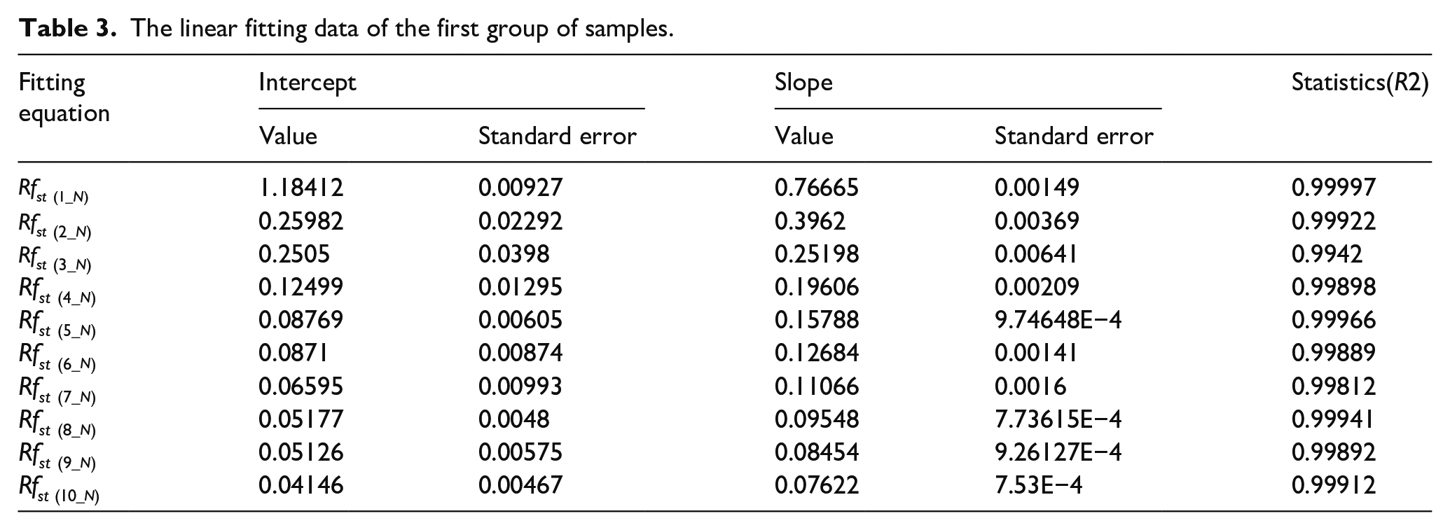
Figure 11 displays that when the voltage is applied to both ends of the course direction, R_st _{(M_N)} is proportional to N under fixing M. The slope and intercept values decrease at a slowing down rate as M increases (can be seen in Table 3).

The slope and intercept values from equations (8)–(9) compared with the linear fitting results in Table 3 are listed in Table 4. It can be seen that the calculated equation of NCR_st _{(M_N)} with RC₃ is closer to the fitting equation Rf_st _{(M_N)} than the CR_st _{(M_N)} without RC₃, which implies that RC₃ exists in the real prepared sensors. The main reason for the existence of RC₃ is the difference in elasticity between the conductive face yarn and the elastic ground yarn in the sensing area, as well as the input tension control of the ground yarn during knitting. Then, the ground yarn at the interlocking position has deviated from the ideal position, which creates a contact space for the conductive face yarn generating RC₃.

Table 4.

The linear fitting and calculating data from the first group of samples.

Equation	Intercept value	Slope value		Intercept value	Slope value
Rf_st (1_N)	1.17485~1.19339	0.76516~0.76814	Rf_st _{(6_N)}	0.07836~0.09584	0.12543~0.12825
NCR_st _{(1_N)}	1.1731	0.7682	NCR_st _{(6_N)}	0.0719	0.1297
CR_st _{(1_N)}	1.1731	0.7682	CR_st _{(6_N)}	0.0677	0.1369
Rf_st _{(2_N)}	0.2369~0.28274	0.39251~0.39989	Rf_st _{(7_N)}	0.05602~0.07588	0.10906~0.11226
NCR_st _{(2_N)}	0.2544	0.3973	NCR_st _{(7_N)}	0.0582	0.1110
CR_st _{(2_N)}	0.5866	0.3841	CR_st _{(7_N)}	0.0530	0.1180
Rf_st (3_N)	0.2107~0.2903	0.24557~0.25839	Rf_st _{(8_N)}	0.04697~0.05657	0.09471~0.09625
NCR_st _{(3_N)}	0.2603	0.2621	NCR_st _{(8_N)}	0.0488	0.0970
CR_st (3_N)	0.2367	0.2646	CR_st _{(8_N)}	0.0432	0.1036
Rf_st (4_N)	0.11204~0.13794	0.19397~0.19815	Rf_st _{(9_N)}	0.04551~0.05701	0.08361~0.08547
NCR_st _{(4_N)}	0.1309	0.1955	NCR_st (9_N)	0.0419	0.0862
CR_st _{(4_N)}	0.1361	0.2018	CR_st _{(9_N)}	0.0362	0.0923
Rf_st _{(5_N)}	0.08164~0.09374	0.15691~0.15885	Rf_st _{(10_N)}	0.03679~0.04613	0.07547~0.07697
NCR_st _{(5_N)}	0.0934	0.1559	NCR_st _{(10_N)}	0.0367	0.0775
CR_st _{(5_N)}	0.0918	0.1631	CR_st _{(10_N)}	0.0311	0.0833

The differences in the slope and intercept values of the fitting and calculating results in Table 4 are shown as below:

When M = 1, the intercept and the slope values of CR_st _{(1_N)} are equal to those of NCR_st _{(1_N)};

When M = 2, the intercept and slope values of CR_st _{(2_N)} are half of those of CR_st _{(1_N)} due to the model. The intercept value of CR_st _{(2_N)} is more than twice of that of NCR_st _{(2_N)}, while the slope value of CR_st _{(2_N)} is lightly smaller to that of NCR_st _{(2_N)};

When M = 3, the differences in the intercept and slope value of CR_st _{(3_N)} and NCR_st _{(3_N)} become smaller, and the intercept value of CR_st _{(3_N)} is slightly smaller to that of NCR_st _{(3_N)}, while the slope value of CR_st _{(3_N)} goes negligibly higher than that of NCR_st _{(3_N)};

When M = 4, the intercept and slope values of CR_st _{(4_N)} become faintly higher than those of CR_st _{(4_N)};

When M ⩾ 5, the intercept values of CR_st _{(M_N)} keep slightly smaller than those of NCR_st _{(M_N)}, while the slope values of CR_st _{(M_N)} remain slightly higher than those of NCR_st _{(M_N)} which also can be deduced by equations (8)–(9).

Relationship between the equivalent resistance and M

The resistances NCR_st _{(M_N)} and CR_st _{(M_N)} of the two models with the specific integer M and N were calculated, respectively, by equations (8)–(9). Fixing N, respectively, analysis of R_st _{(M_N)}, CR_st _{(M_N)}, and NCR_st _{(M_N)} was performed by plotting data where the integer M changes from 1 to 10, as shown in Figure 12. It is found that R_st _{(M_N)}, CR_st _{(M_N)}, and NCR_st _{(M_N)} decrease at a reducing rate as M increases. In addition, Figure 12(b)–(e) is the enlarged view of some parts of data curves in Figure 12(a) to explicit the curves. It can be gotten that when M ⩾ 5, CR_st _{(M_N)} is always higher than NCR_st _{(M_N)}, and the difference gradually increases as the increase of N. Also, NCR_st _{(M_N)} is closer to the experimental value R_st _{(M_N)} than CR_st _{(M_N)}.

Figure 12.

Fixing the number of conductive wales N, the comparison of the experimental and calculated data of the first group of samples: (a) Raw plots of the experimental data and calculated data and (b–e) enlarged views of the corresponding parts in (a), respectively.

To further verify the correctness of the model, Table 2 was analyzed by the data curves of R_st _{(M_N)}, CR_st _{(M_N)}, and NCR_st _{(M_N)}, where N equals 50, 100, and 150, respectively, as depicted in Figure 13. Similarly, CR_st _{(M_N)} is always higher than NCR_st _{(M_N)} for specific M and N, and the difference gradually grows as the increase of N and decreases as the increase of M.

Figure 13.

Fixing the number of conductive wales N, the comparison of the experimental and calculated data of the second group of samples: (a) Plots of the experimental data and calculated data when M equals from 5 to 35 with the interval of 5 and (b) plots of the experimental data and calculated data when M equals to other values.

Comparison of the two established resistive network models

Finally, to compare the two established models, three-dimensional surface plots of the calculated resistances, NCR_st _{(M_N)} and CR_st _{(M_N)}, were made according to equations (8)–(9). Here M is from 7 to 500, and N is from 1 to 500, as displayed in Figure 14 containing the projections on the coordinate planes (Figure 14(b)–(d) and (f)–(h)). For the two models, the various forms of the calculated resistances with M and N are the same as those in Figure 13. The resistances decrease non-linearly as the increase of M (see projections on the x-z plane in Figure 14(b) and (f)) and increase linearly as the increase of N (see projections on the y-z plane in Figure 14(c) and (g)). The color bars (see Figure 14(d) and (h)) illustrate that the value range of CR_st _{(M_N)} is slightly more extensive than that of NCR_st _{(M_N)}. The projections on the x-y plane in Figure 14(d) and (h) indicate that the difference between CR_st _{(M_N)} and NCR_st _{(M_N)} becomes slightly small as the increase of M where the resistance value approaches zero.

Figure 14.

When M ⩾ 7, N ⩾ 1, the three-dimensional surface plots of the resistance, M and N of the two models and their projections on each plane: (a) Three-dimensional surface plots of the resistive network model with RC₃ and the corresponding projections (b–d) and (e) three-dimensional surface plots of the resistive network model without RC₃ and the corresponding projections (f–h).

Conclusion

In the present study, two resistive network models of the weft-knitted strain sensor with the plating stitch have been established accordingly. The first model was based on the jamming and interlocking contact resistances, while the second one only focused on the jamming contact resistances, which can improve the existing static relaxation resistive network models.^12,13,16,17 In the case of applying voltage along the two ends of the course, the theoretical resistance calculation of the corresponding model was performed through using a series of equivalent transformations to simplify the model to the final easy-to-solve resistive network. It can be found that the two established resistive network models both can be simplified to a series-parallel resistive network connected in series along course direction and parallel along the wale direction, which is consistent with the conclusions of other researchers.^16,17

Finally, the correctness and usability of the two models were verified by experiments and calculations based on the models. It can be concluded that both models can predict the change law of the equivalent resistance with the number of conductive courses and wales, that is, the equivalent resistance increases with the number of wales and decreases with the number of courses, which coincides with the discoveries of other investigators.^16,18

In addition, the calculating resistances of the first model are closer to the experimental data and smaller than those of the second model. Moreover, the difference will become smaller as the number of courses increases, which reflects that the jamming contact resistance has a more considerable influence on the resistive network than the interlocking contact resistance. Furthermore, the two established resistive network models can be further used to analyze the effect of different contact and length-related resistances on the total equivalent resistance by numerical analysis.

Admittedly, because it is challenging to calculate the contact resistances in building the models theoretically, the determining of the contact resistances in verifying the model depends on the experiment. Moreover, this article only investigates the resistance network model of the knitted strain sensor under static relaxation. However, when the sensor works, the corresponding resistance network dynamically changes, so the next article in this series will deal with the resistance network model under the elongation along course direction.

Supplemental Material

Figure_S1 – Supplemental material for Resistive network model of the weft-knitted strain sensor with the plating stitch-Part 1: Resistive network model under static relaxation

Supplemental material, Figure_S1 for Resistive network model of the weft-knitted strain sensor with the plating stitch-Part 1: Resistive network model under static relaxation by Yujing Zhang and Hairu Long in Journal of Engineered Fibers and Fabrics

Supplemental Material

Figure_S10 – Supplemental material for Resistive network model of the weft-knitted strain sensor with the plating stitch-Part 1: Resistive network model under static relaxation

Supplemental material, Figure_S10 for Resistive network model of the weft-knitted strain sensor with the plating stitch-Part 1: Resistive network model under static relaxation by Yujing Zhang and Hairu Long in Journal of Engineered Fibers and Fabrics

Supplemental Material

Figure_S2 – Supplemental material for Resistive network model of the weft-knitted strain sensor with the plating stitch-Part 1: Resistive network model under static relaxation

Supplemental material, Figure_S2 for Resistive network model of the weft-knitted strain sensor with the plating stitch-Part 1: Resistive network model under static relaxation by Yujing Zhang and Hairu Long in Journal of Engineered Fibers and Fabrics

Supplemental Material

Figure_S3 – Supplemental material for Resistive network model of the weft-knitted strain sensor with the plating stitch-Part 1: Resistive network model under static relaxation

Supplemental material, Figure_S3 for Resistive network model of the weft-knitted strain sensor with the plating stitch-Part 1: Resistive network model under static relaxation by Yujing Zhang and Hairu Long in Journal of Engineered Fibers and Fabrics

Supplemental Material

Figure_S4 – Supplemental material for Resistive network model of the weft-knitted strain sensor with the plating stitch-Part 1: Resistive network model under static relaxation

Supplemental material, Figure_S4 for Resistive network model of the weft-knitted strain sensor with the plating stitch-Part 1: Resistive network model under static relaxation by Yujing Zhang and Hairu Long in Journal of Engineered Fibers and Fabrics

Supplemental Material

Figure_S5 – Supplemental material for Resistive network model of the weft-knitted strain sensor with the plating stitch-Part 1: Resistive network model under static relaxation

Supplemental material, Figure_S5 for Resistive network model of the weft-knitted strain sensor with the plating stitch-Part 1: Resistive network model under static relaxation by Yujing Zhang and Hairu Long in Journal of Engineered Fibers and Fabrics

Supplemental Material

Figure_S6 – Supplemental material for Resistive network model of the weft-knitted strain sensor with the plating stitch-Part 1: Resistive network model under static relaxation

Supplemental material, Figure_S6 for Resistive network model of the weft-knitted strain sensor with the plating stitch-Part 1: Resistive network model under static relaxation by Yujing Zhang and Hairu Long in Journal of Engineered Fibers and Fabrics

Supplemental Material

Figure_S7 – Supplemental material for Resistive network model of the weft-knitted strain sensor with the plating stitch-Part 1: Resistive network model under static relaxation

Supplemental material, Figure_S7 for Resistive network model of the weft-knitted strain sensor with the plating stitch-Part 1: Resistive network model under static relaxation by Yujing Zhang and Hairu Long in Journal of Engineered Fibers and Fabrics

Supplemental Material

Figure_S8 – Supplemental material for Resistive network model of the weft-knitted strain sensor with the plating stitch-Part 1: Resistive network model under static relaxation

Supplemental material, Figure_S8 for Resistive network model of the weft-knitted strain sensor with the plating stitch-Part 1: Resistive network model under static relaxation by Yujing Zhang and Hairu Long in Journal of Engineered Fibers and Fabrics

Supplemental Material

Figure_S9 – Supplemental material for Resistive network model of the weft-knitted strain sensor with the plating stitch-Part 1: Resistive network model under static relaxation

Supplemental material, Figure_S9 for Resistive network model of the weft-knitted strain sensor with the plating stitch-Part 1: Resistive network model under static relaxation by Yujing Zhang and Hairu Long in Journal of Engineered Fibers and Fabrics

Supplemental Material

Supplementary_Materials – Supplemental material for Resistive network model of the weft-knitted strain sensor with the plating stitch-Part 1: Resistive network model under static relaxation

Supplemental material, Supplementary_Materials for Resistive network model of the weft-knitted strain sensor with the plating stitch-Part 1: Resistive network model under static relaxation by Yujing Zhang and Hairu Long in Journal of Engineered Fibers and Fabrics

Footnotes

Declaration of conflicting interests

The author(s) declared no potential conflicts of interest with respect to the research, authorship, and/or publication of this article.

Funding

The author(s) received no financial support for the research, authorship, and/or publication of this article.

ORCID iD

Yujing Zhang

Supplemental material

Supplemental material for this article is available online.

References

Miao

Niu

, et al. Human motion recognition of knitted flexible sensor in walking cycle. Sensors 2020; 20(35): 1–14.

Tian

, et al. Multiscale disordered porous fibers for self-sensing and self-cooling integrated smart sportswear. Acs Nano 2020; 14: 559–567.

Sun

Tian

Sun

, et al. Stretchable conductive fibers of ultrahigh tensile strain and stable conductance enabled by a worm-shaped graphene microlayer. Nano Letters 2019; 19: 6592–6599.

Seyedin

Zhang

Naebe

, et al. Textile strain sensors: a review of the fabrication technologies, performance evaluation and applications. Mater Horiz 2019; 6: 219–249.

Park

Ahn

Sun

, et al. Highly bendable and rotational textile structure with prestrained conductive sewing pattern for human joint monitoring. Adv Funct Mater 2019; 29(10): 1–12.

Rozevika

Katashev

Okss

, et al. On the monitoring of breathing volume, using textile strain gauges. In: Lhotska

Sukupova

Lackovic

, et al. (eds) World congress on medical physics and biomedical engineering 2018 IFMBE Proceedings, Cham, Switzerland: Springer, 2019, pp. 921–925.

Raji

Miao

Wan

, et al. Knitted piezoresistive smart chest band and its application for respiration patterns assessment. J Eng Fibers Fabr 2019; 14(4): 1–14.

Han

Miao

Chen

, et al. Research on finger movement sensing performance of conductive gloves. J Eng Fibers Fabr 2019; 14: 1–7.

Miao

Raji

RK.

Flexible knitted sensing device for identifying knee joint motion patterns. Smart Mater Struct 2019; 28(11): 1–9.

10.

Yang

Pan

, et al. Conductive cotton fabrics for motion sensing and heating applications. Polymers 2018; 10(6): 1–12.

11.

Yang

Pang

Han

, et al. Graphene textile strain sensor with negative resistance variation for human motion detection. Acs Nano 2018; 12: 9134–9141.

12.

Zhang

Relationship between mechanical-electrical properties and fabric structures made from intrinsically conductive fibers. In: X

Tao

(ed) Handbook of smart textiles, Singapore: Springer, 2015, pp. 719–737.

13.

Zhang

Tao

Wang

, et al. Electro-mechanical properties of knitted fabric made from conductive multi-filament yarn under unidirectional extension. Text Res J 2005; 75: 598–606.

14.

Liu

Ding

, et al. Mechanical-electrical analysis of length-related resistance and contact resistance of conductive knitted fabrics. Text Res J 2012; 82: 2062–2070.

15.

Tao

, et al. Design of a conductive fabric network by the sheet resistance method. Text Res J 2011; 81: 1568–1577.

16.

Wan

, et al. A resistive network model for conductive knitting stitches. Text Res J 2010; 80: 935–947.

17.

Wang

Long

Soltanian

, et al. Mechanical—electrical properties of knitted wearable sensors: part I—theory. Text Res J 2014; 84: 3–15.

18.

Wang

Long

Soltanian

, et al. Electro-mechanical properties of knitted wearable sensors: part 2-parametric study and experimental verification. Text Res J 2014; 84: 200–213.

19.

Xie

Long

HR.

Investigation on the relation between structure parameters and sensing properties of knitted strain sensor under strip biaxial elongation. J Eng Fibers Fabr 2015; 10: 166–178.

20.

Xie

Long

HR.

Equivalent resistance calculation of knitting sensor under strip biaxial elongation. Sens Actuator A-phys 2014; 220: 118–125.

21.

Liu

Tong

Yang

, et al. Smart E—textile: resistance properties of conductive knitted fabric—single pique. Text Res J 2017; 87: 1669–1684.

22.

Liu

Yang

Zhao

, et al. The impact of float stitches on the resistance of conductive knitted structures. Text Res J 2016; 86: 1455–1473.

23.

Atalay

Tuncay

Husain

, et al. Comparative study of the weft-knitted strain sensors. J Ind Text 2017; 46: 1212–1240.

24.

Wang

Long

HR.

Research on wearable sensors based on knitted fabrics with silver plating fiber. Adv Mater Res-switz 2011; 331: 36–39.

25.

Hong

Pan

Zhe

, et al. A large-strain weft-knitted sensor fabricated by conductive UHMWPE/PANI composite yarns. Sens Actuator A-phys 2016; 238: 307–316.

26.

Peirce

FT.

Geometrical principles applicable to the design of functional fabrics. Text Res J 1947; 17: 123–147.

27.

Holm

Electric contacts: theory and application. 4th ed. New York: Springer Science & Business Media, 1967.

28.

Alexander

Sadiku

MNO

. Part1: DC circuits fundamentals of electric circuits. 6th ed. New York: McGraw-Hill Education, 2017, pp. 3–77.

Supplementary Material

Please find the following supplemental material available below.

For Open Access articles published under a Creative Commons License, all supplemental material carries the same license as the article it is associated with.

For non-Open Access articles published, all supplemental material carries a non-exclusive license, and permission requests for re-use of supplemental material or any part of supplemental material shall be sent directly to the copyright owner as specified in the copyright notice associated with the article.

0.00 MB

0.23 MB

0.18 MB

0.59 MB

1.05 MB

0.86 MB

0.61 MB

0.89 MB

0.60 MB

0.80 MB

2.96 MB

Resistive network model of the weft-knitted strain sensor with the plating stitch-Part 1: Resistive network model under static relaxation

Abstract

Keywords

Introduction

The basic unit of the weft-knitted strain sensor with the plating stitch

Weft jacquard plating technology

The definitions of the concerning contact resistances

Establishment and theoretical calculation of the resistive network models under static relaxation

Resistive network model with RC1,RC2,RC3, and RC4

Resistive network model with RC1, RC2, and RC4

Experiment and model calculation

Materials, sample preparation, and testing set

Sample specification design and experimental data

Calculations of the two resistive network models

Results and discussion

Relationship between the equivalent resistance and N

Relationship between the equivalent resistance and M

Comparison of the two established resistive network models

Conclusion

Supplemental Material

Figure_S1 – Supplemental material for Resistive network model of the weft-knitted strain sensor with the plating stitch-Part 1: Resistive network model under static relaxation

Supplemental Material

Figure_S10 – Supplemental material for Resistive network model of the weft-knitted strain sensor with the plating stitch-Part 1: Resistive network model under static relaxation

Supplemental Material

Figure_S2 – Supplemental material for Resistive network model of the weft-knitted strain sensor with the plating stitch-Part 1: Resistive network model under static relaxation

Supplemental Material

Figure_S3 – Supplemental material for Resistive network model of the weft-knitted strain sensor with the plating stitch-Part 1: Resistive network model under static relaxation

Supplemental Material

Figure_S4 – Supplemental material for Resistive network model of the weft-knitted strain sensor with the plating stitch-Part 1: Resistive network model under static relaxation

Supplemental Material

Figure_S5 – Supplemental material for Resistive network model of the weft-knitted strain sensor with the plating stitch-Part 1: Resistive network model under static relaxation

Supplemental Material

Figure_S6 – Supplemental material for Resistive network model of the weft-knitted strain sensor with the plating stitch-Part 1: Resistive network model under static relaxation

Supplemental Material

Figure_S7 – Supplemental material for Resistive network model of the weft-knitted strain sensor with the plating stitch-Part 1: Resistive network model under static relaxation

Supplemental Material

Figure_S8 – Supplemental material for Resistive network model of the weft-knitted strain sensor with the plating stitch-Part 1: Resistive network model under static relaxation

Supplemental Material

Figure_S9 – Supplemental material for Resistive network model of the weft-knitted strain sensor with the plating stitch-Part 1: Resistive network model under static relaxation

Supplemental Material

Supplementary_Materials – Supplemental material for Resistive network model of the weft-knitted strain sensor with the plating stitch-Part 1: Resistive network model under static relaxation

Footnotes

Declaration of conflicting interests

Funding

ORCID iD

Supplemental material

References

Supplementary Material

Resistive network model with RC₁,RC₂,RC₃, and RC₄

Resistive network model with RC₁, RC₂, and RC₄