Methods for improving the accuracy of Commission Internationale de L’Eclairage tristimulus values of object color by calculation – Part I: Improvement on measurement bandpass and intervals

Abstract

Color is one of the most important appearance properties of objects. To digitize color, measuring and calculating tristimulus values are the most basic work besides obtaining reflectance spectrum. However, the accuracy of tristimulus values varies with instruments, measuring, and calculation methods. Textiles and some other application of color demand high color quality due to their special utilization. The series of our studies aim to analyze and evaluate some mathematical solutions in order to improve the accuracy of tristimulus values. The studies include two parts: (1) Part I concentrates on measurement bandpass and intervals and their corresponding improvement algorithms, (2) Part II focuses on the influence of measurement ranges and their truncation errors and some algorithms to overcome the truncation errors. In Part I (current article), measurement errors caused by bandpass and test intervals in the spectrophotometer are analyzed. Then, algorithms including two bandpass corrections (3-point correction and 5-point correction), three interpolations (third-order polynomial interpolation Lagrange and Spline, a fifth-order polynomial interpolation Sprague), two Oleari deconvolution methods (zero- and second-order), and three optimization weighting table methods (ASTM Table 6, Table LLR, and Table LWL) are studied systemically by programming MATLAB software and basing on measuring the spectral reflectance of 1301 chips in Munsell Color Book with Commission Internationale de L’Eclairage (CIE) 1964 color-matching functions and D₆₅ standard illuminant. The results show that all algorithms mentioned above yield very positive effects, and among them, Table LWL performs best with reducing the bandpass error and intervals error to 7‰ of its original error and is recommended.

Introduction

Tristimulus values (TSVs) are the basic parameters describing color quantitatively; they can be transformed to other colorimetric parameters used in color management and color communication. Commission Internationale de L’Eclairage (CIE) TSVs of a color are the qualities of three primary colors needed to match the color, defined as integrals over the spectral range 360–830 nm as shown in equation (1) by CIE ¹

$$\{\begin{array}{l}X=k\underset{\lambda }{\int }R\left(\lambda \right)S\left(\lambda \right)\overline{x}\left(\lambda \right)d\lambda \\ Y=k\underset{\lambda }{\int }R\left(\lambda \right)S\left(\lambda \right)\overline{y}\left(\lambda \right)d\lambda \\ Z=k\underset{\lambda }{\int }R\left(\lambda \right)S\left(\lambda \right)\overline{z}\left(\lambda \right)d\lambda \\ k=\frac{100}{\underset{\lambda }{\int }S\left(\lambda \right)\overline{y}\left(\lambda \right)d\lambda }\end{array}$$

(1)

where X, Y, and Z are the CIE TSVs and will be presented by V or XYZ in this article; R(λ) is the spectral reflectance; S(λ) is the relative spectral distribution of illuminant; $\overline{x}(\lambda )$ , $\overline{y}\left(\lambda \right)$ , and $\overline{z}(\lambda )$ are the color-matching functions and will be presented by $\overline{v}(\lambda )$ later; and k is a normalized factor to make Y = 100 for the illuminant.

Since the integrands in equation (1) have no analytical equivalent expressions, CIE published a standard method for computing these integrals, that is to calculate the numerical summation from 360 to 830 nm at wavelength intervals Δλ = 1 nm as shown in equation (2), where the R(λ) should be measured using a symmetrical triangular or trapezoidal bandpass with half-wave width equal to 1 nm¹

$$\{\begin{array}{l}V=k\sum _{\lambda }R\left(\lambda \right)S\left(\lambda \right)\overline{v}\left(\lambda \right)d\lambda \\ k=\frac{100}{\sum _{\lambda }S\left(\lambda \right)\overline{y}\left(\lambda \right)d\lambda }\end{array}$$

(2)

In practical application, many spectrophotometers for color measuring (spectrocolorimeter) can only measure the spectral reflectance in narrower band like 360–750 nm or 400–700 nm and with larger intervals like 10 nm or even 20 nm. If we use these data to calculate the TSVs, it will yield a calculation error since the data do not meet CIE’s requirement of 360-830 nm and 1-nm intervals. This error will further mislead the subsequent computation and comparison of colorimetric parameters. The ideal solution to keep accuracy is of course to improve the performance of spectrophotometers. However, the solution will need to change some key optical hardwares and increase the cost greatly; what is more, it still cannot solve the current problem of the existing spectrophotometers widely used in factories and laboratories.

At present, the inconsistent calculation methods caused by the measurement range and intervals lead to a discrepancy of TSVs of the same sample when calculating with different intervals, ranges, or algorithms. Therefore, it is necessary to develop a calculation method for accurate TSVs; then, it can be properly used in color communication and management, such as color reproduction, color quality control, color difference evaluation, metamerism, and computer color matching, color duplication, and so on, so as to reduce the error and avoid needless and excessive operations caused by error. This investigation focuses on the algorithms to improve the accuracy of TSVs by reducing the errors caused by larger measurement intervals and narrower band range. Part I (current article) is about measurement intervals and Part II (forthcoming article) is on measurement ranges.

When measurement intervals are greater than 1 nm, there will be another joint problem of bandpass. To solve the problem of measurement intervals and bandwidth being greater than 1 nm, experts proposed many algorithms to improve the accuracy. Among these methods, the mainly recognized are the following: SS bandpass correction method, ² Fairman correction method,^3,4 interpolation methods,^5,6 Oleari methods, ⁷ American Society of Testing Materials (ASTM) tables, ⁸ Table Li-Luo-Rigg (LLR), ⁹ Table Li-Wang-Luo (LWL), ¹⁰ and so on. In this article, these methods are employed and compared by programming MATLAB software and statistical analysis in order to obtain the best solution.

Measurement errors of spectrophotometer

The deviation between the value measured by the instrument and the true/standard value is the measurement error of the instrument. For convenient expression, the measurement errors of normal spectrophotometers are divided into three categories: measurement bandpass error, measurement intervals error, and measurement range error. The errors of measurement intervals and range are easy to be understood; hence, the bandpass error is further explained only.

Because of the performance of the monochromator in the spectrophotometer, when measuring the reflectance at a specific wavelength $\lambda$ , the light from the slit is not exactly the light at $\lambda$ , but a combined light beam contains ±A $\lambda$ (A is an arbitrary constant). Thus, all spectrophotometers measure reflectance of each measurement wavelength with a finite bandwidth, the bandwidth being chosen so as to pass a reasonable amount of power to the detector. For monochrome light, the narrower the slit, the smaller the bandwidth, the higher purity of light, but the weaker the intensity. Therefore, the slit cannot be reduced unlimitedly, the minimum width of the slit depends on the minimum light energy that the detector can accurately measure.

Assume the relative strength of the light at wavelength $\lambda$ is 100, at wavelength Δ ${\lambda }_1$ being shorter and Δ ${\lambda }_2$ longer than that at $\lambda$ by 50, then Δλ = Δλ₁ + Δλ₂ is the spectral bandwidth. ¹¹ If we use $R(\lambda )$ to represent the pure 1-nm interval’s reflectance, and $\tilde{R}(\lambda )$ to stand for the measured 10- or 20-nm interval’s reflectance with the bandwidth, the measured values $\tilde{R}(\lambda )$ at any bandpass are the integral of the product of the instrument function $P_i(\lambda )$ and the true values $R(\lambda )$ over the range of the bandwidth. The relationship between these two kinds of reflectance is shown in equation (3)

$${\tilde{R}}_i\left(\lambda \right)=\underset{a}{\overset{b}{\int }}{P}_i\left(\lambda \right)R\left(\lambda \right)d\lambda$$

(3)

where, $P_i\left(\lambda \right)$ is the instrumental function or bandpass function, scaled by equation (4)

$$\underset{a}{\overset{b}{\int }}{P}_i\left(\lambda \right)d\lambda =1$$

(4)

Many spectrophotometers have the bandpass function with a symmetrical triangular shape, as shown in Figure 1. Then $P_i\left(\lambda \right)$ can be expressed by equation (5).

$$P_i\left(\lambda \right)=\left\{\begin{array}{cc}\frac{\lambda -{\lambda }_{i-1}}{{\left(\Delta \lambda \right)}^2}& {\lambda }_{i-1}\le \lambda \le {\lambda }_i\\ \frac{{\lambda }_{i+1}-\lambda }{{\left(\Delta \lambda \right)}^2}& {\lambda }_i\le \lambda \le {\lambda }_{i+1}\\ 0& \lambda <{\lambda }_{i-1},\lambda >{\lambda }_{i+1}\end{array}\right\}$$

(5)

Figure 1.

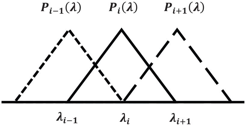
The spectral bandpass function. ¹⁰

All spectral data measured from the spectrophotometer have a certain bandwidth. If it is not processed mathematically, the calculated TSVs will be in error. The measurement intervals should be equal to the bandwidth in order to keep the result more accuracy.^12,13 And the error caused by bandwidth is usually much larger than that caused by the measurement intervals on the order of magnitude. ¹

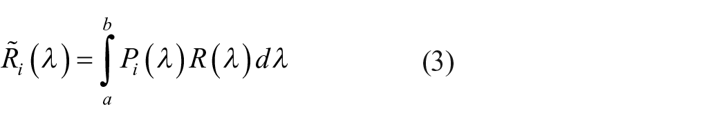
As a result of the presence of bandwidth, the measured $\tilde{R}(\lambda )$ is a kind of average of the true R(λ) near λ. If the spectral reflectance function R(λ) is a linear function over the range of $[{\lambda }_{i-1},{\lambda }_{i+1}]$ , the measured value obtained by the equation integral is equal to the true value. If the spectral reflectance function is concave in the range, the measured value obtained by the integral is larger than the true value, and vice versa.

Methods for higher accuracy of TSVs

In view of the status of the existing and commonly used 10-nm interval instruments at present, we seek to make up the deficiencies of the instruments through mathematical methods so as to improve the accuracy of the TSVs.

Reduce bandpass error by bandpass corrections

CIE points that ¹ the bandwidth of the instruments which is used to yield the spectral reflectance for TSVs computation should be 5 nm or less, otherwise the bandwidth should be corrected by available methods. The mainly used bandpass correction methods are SS method proposed by Stearns & Stearns ² and the Fairman method ⁴ recommended by ASTM. ³

Stearns & Stearns realized that the measured reflectance R_m,λ was a function of the true spectral reflectance R_s,λ within the bandpass. The measurement bandpass would be designated by the reflectance at wavelength λ₀, the next-previous λ₋₁, and the next-higher bandpass λ₁

$$R_{m,0}=a_{-1}{R}_{s,-1}+a_0{R}_{s,0}+a_1{R}_{s,1}$$

(6)

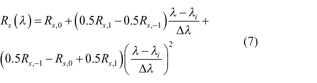
They assumed that the true spectral reflectance R_s was a quadratic passing through the three adjacent points (λ_i−1, R_s,₋₁), (λ_i, R_s,₀), and (λ_i+1, R_s,₁); this quadratic could be presented as equation (7)

$$\begin{array}{l}{R}_s\left(\lambda \right)=R_{s,0}+\left(0.5R_{s,1}-0.5R_{s,-1}\right)\frac{\lambda -{\lambda }_i}{\Delta \lambda }+\\ \left(0.5R_{s,-1}-R_{s,0}+0.5R_{s,1}\right){\left(\frac{\lambda -{\lambda }_i}{\Delta \lambda }\right)}^2\end{array}$$

(7)

The relationship between R_m,λ (have the same means with $\tilde{R}(\lambda )$ ) and R_s,λ (have the same means with $R(\lambda )$ ) conforms to equation (3); then, they substituted equation (7) into equation (3), getting equation (8)

$$R_{m,0}=\frac{1}{12}{R}_{s,-1}+\frac{5}{6}{R}_{s,0}+\frac{1}{12}{R}_{s,1}$$

(8)

This equation can be solved for R_s,0

$$R_{s,0}=-0.1R_{s,-1}+1.2R_{m,0}-0.1R_{s,1}$$

(9)

Now, the right-hand side of this equation is in terms of both measured and true spectral reflectance. Then, Stearns & Stearns used the approximation theory, substituting the measured reflectance (known) into this equation for the true reflectance (unknown), thus leading to equation (10)

$$R_{s,0}=-0.1R_{m,-1}+1.2R_{m,0}-0.1R_{m,1}$$

(10)

So, the final form of SS correction method is shown in equation (11)

$$\begin{array}{l}{R}_{s,1}=\left(1+\alpha \right)R_{m,1}-\alpha R_{m,2}\\ R_{s,i}=-\alpha R_{m,i-1}+\left(1+\alpha \right)R_{m,i}-\alpha R_{m,i+1}\\ R_{s,n}=\left(1+\alpha \right)R_{m,n}-\alpha R_{m,n-1}\end{array}$$

(11)

where $R_{s,i}$ is the reflectance at the wavelength i after correction. $R_{m,i}$ is the reflectance at the wavelength i before correction. The parameter α is initially 0.1 in equation (10), after several modifications, α = 0.083 suggested by Venable is considered to be more reasonable and adopted ever since. ⁴

The Fairman correction method has the same principle with SS correction, and this time assume the quadratic passing through five adjacent points. The Fairman correction method can be found in equations (12)–(14). The first point and the last point of the reflectance use equation (12), the second point and the second last point use equation (13), and the middle points use equation (14)

$$\begin{array}{l}{R}_{s,1}=R_{m,1}\\ R_{s,n}=R_{m,n}\end{array}$$

(12)

$$\begin{array}{l}{R}_{s,2}=-0.10R_{m,1}+1.21R_{m,2}-\\ 0.12R_{m,3}+0.01R_{m,4}\\ R_{s,n-1}=0.01R_{m,n-3}-0.12R_{m,n-2}+\\ 1.21R_{m,n-1}-0.10R_{m,n}\end{array}$$

(13)

$$\begin{array}{l}{R}_{s,i}=0.01R_{m,i-2}-0.12R_{m,i-1}+1.22R_{m,i}-\\ 0.12R_{m,i+1}+0.01R_{m,i+2}\end{array}$$

(14)

Reduce measurement intervals error

The simplest and most primitive method for calculating the TSVs is the direct selection method, that is, according to the intervals of the measured reflectance, the weighting coefficients at corresponding wavelength are extracted from the weighting table of 1 nm given by CIE. This calculation method exists both the bandpass error and the intervals error, and the errors are large and increase significantly with the increase of wavelength intervals.

For spectral reflectance with greater measurement intervals than 1 nm, there are three types of methods to improve the accuracy of TSVs computing. One is the interpolation method, the second is the Oleari method, and the third is the optimization weighting table method.

Interpolation methods

The interpolation method is to insert data to make the bandpass-corrected reflectance into 1-nm-interval in order to content with the CIE’s demand of 1-nm intervals for decreasing the intervals error. Before interpolation, the measured $\tilde{R}(\lambda )$ with bandpass should be corrected first to eliminate the bandpass error.

In regard to the interpolation methods, CIE15:2004 ⁵ recommends third-order polynomial interpolation (Lagrange), cubic Spline interpolation, and a fifth-order Sprague interpolation. CIE167:2005 ⁶ recommends that empirical data should be interpolated by a fifth-order Sprague equation when the independent variable is tabulated at uniform intervals, and by a cubic Spline method when the intervals are not uniform. The Table 5 in ASTM E308-15 ⁸ uses the Lagrange interpolation method. ¹⁴

This article combines the bandpass correction with the third-order (Lagrange, Spline) and the fifth-order (Sprague) polynomial interpolation to calculate and make intercomparison.

Oleari methods

Oleari methods were proposed by Oleari ⁷ in 2000 and simplified by Prof. Li et al. ¹⁵ by providing weighting tables in 2011. Oleari proposed to use a deconvolution method to determine the reflectance of an object at 1-nm intervals, which is similar to the interpolation method, that is, the reflectance of the larger intervals is deconvolved to that of 1-nm intervals by local-power expansion. While Oleari ⁷ did not compute the weighting table, thus, the original method is not convenient to use for calculating TSVs repeatedly for different objects. Li et al. ¹⁵ derived weighting tables of zero-order and second-order forms according to Oleari’s work. The zero-order weighting tables (OWT0) should be used with the bandpass-corrected reflectance, while the second-order weighting table (OWT2) can be adopted with the measured reflectance directly.

Optimization weighting table methods

Optimization weighting table methods take into account the influence of bandpass and intervals simultaneously to produce weighting tables with different intervals, different illuminants, and different observers. When calculating TSVs with the help of optimization weighting table, there is no need to conduct bandpass correction and interpolation, just using the weight coefficient W in the optimized weighting table to replace $S(\lambda )\overline{v}(\lambda )$ in equation (2) directly.

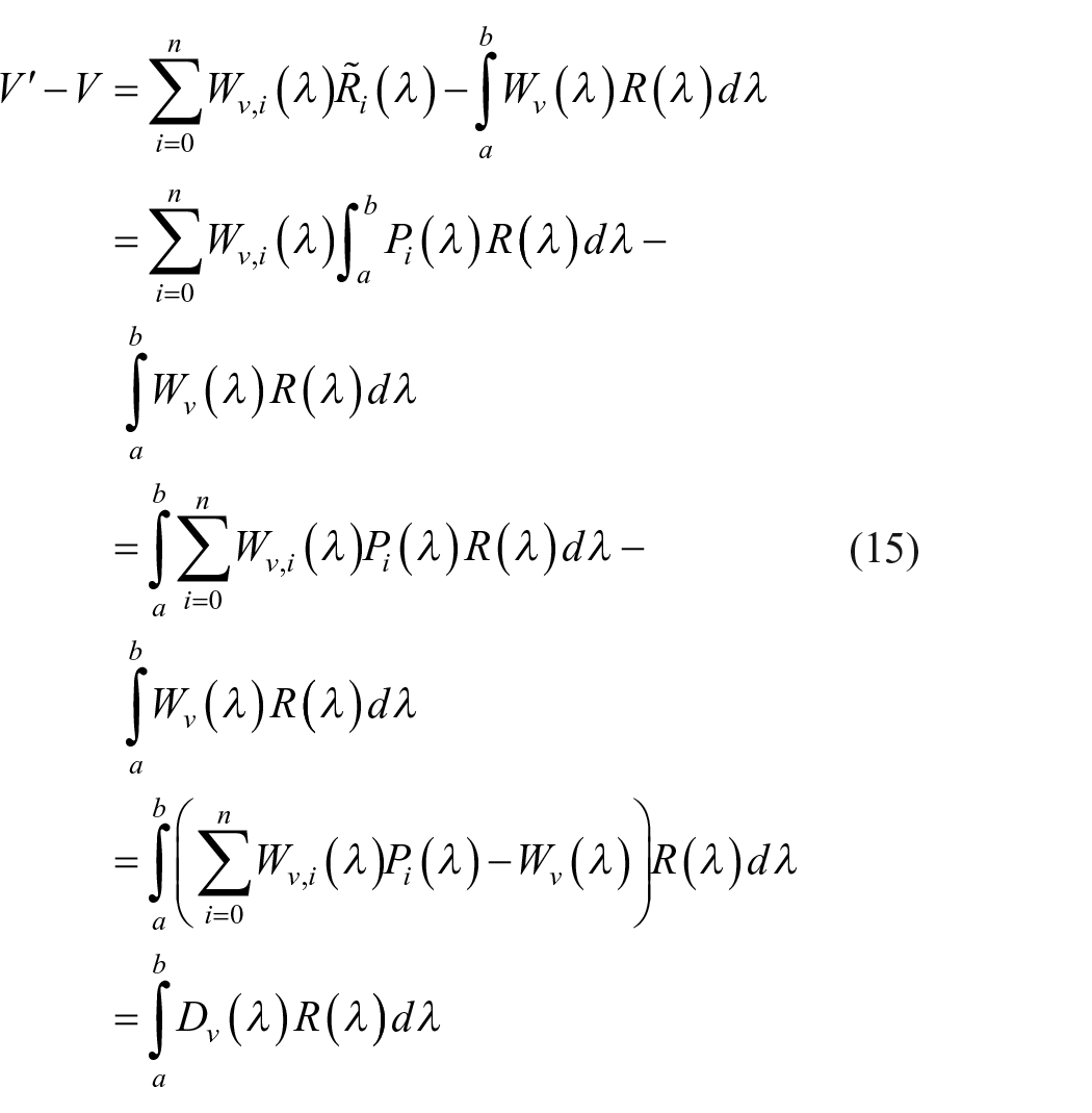
The optimization method ¹⁶ generates weighting tables by minimizing the difference between the calculated TSV V′ and the CIE standard TSV V. V′ is calculated by the 10-nm or 20-nm interval reflectance with the corresponding bandwidth. The process is shown in equation (15). This method does not process the reflectance $\tilde{R}\left(\lambda \right)$ of the non-1-nm interval with bandwidth, just calculates the TSVs using the new weighting table solved by the optimization algorithm directly

$$\begin{array}{c}{V}^{\prime }-V=\sum _{i=0}^n{W}_{v,i}\left(\lambda \right){\tilde{R}}_i\left(\lambda \right)-\underset{a}{\overset{b}{\int }}{W}_v\left(\lambda \right)R\left(\lambda \right)d\lambda \\ =\sum _{i=0}^n{W}_{v,i}\left(\lambda \right){\int }_a^b{P}_i\left(\lambda \right)R\left(\lambda \right)d\lambda -\\ \underset{a}{\overset{b}{\int }}{W}_v\left(\lambda \right)R\left(\lambda \right)d\lambda \\ =\underset{a}{\overset{b}{\int }}\sum _{i=0}^n{W}_{v,i}\left(\lambda \right)P_i\left(\lambda \right)R\left(\lambda \right)d\lambda -\\ \underset{a}{\overset{b}{\int }}{W}_v\left(\lambda \right)R\left(\lambda \right)d\lambda \\ =\underset{a}{\overset{b}{\int }}\left(\sum _{i=0}^n{W}_{v,i}\left(\lambda \right)P_i\left(\lambda \right)-W_v\left(\lambda \right)\right)R\left(\lambda \right)d\lambda \\ =\underset{a}{\overset{b}{\int }}{D}_v\left(\lambda \right)R\left(\lambda \right)d\lambda \end{array}$$

(15)

The main optimization methods are weighting table Table 6 suggested by ASTM E308-15, ⁸ the optimum weighting table Table LLR, ⁹ and the least-squares method optimized table Table LWL ¹⁰ proposed by Li et al. in 2004 and 2016 separately.

ASTM Table 6 (Table 6) carries out the optimization weighting table by the iterative method. At present, ASTM provides 36 weighting tables in 360-780 nm range at 10- and 20-nm intervals under illuminates of A, C, D, and F. Since there is no relative paper publish the detail of its algorithm, the specific processing method has been lost. ¹⁰ Therefore, this method can only be used for the given illuminates and observers.

Table LLR and Table LWL provide simple ways to generate weighing tables according to equation (15); hence, it is easy to derive other tables for any intervals, any ranges, any illuminants, and any observers.

Comparing the above three methods, the interpolation method and the Oleari OWT0 are only considering wavelength intervals, so they should be used with the bandpass-corrected $\tilde{R}(\lambda )$ . The optimization weighting tables and the Oleari OWT2 have incorporated the bandpass factors and should be used with the measured reflectance $\tilde{R}(\lambda )$ of certain wavelength intervals with bandwidth.

Experimental

Selection of samples

1301 chips from the Munsell Color Book (Matt version) were selected as the color samples in this study. These 1301 samples give a good coverage of Hue, Value, and Chroma in color space. Figure 2 shows them in chromatic coordinates, and Figure 3 gives a picture of color chips in the Munsell Color Book with H = 5YR.

Figure 2.

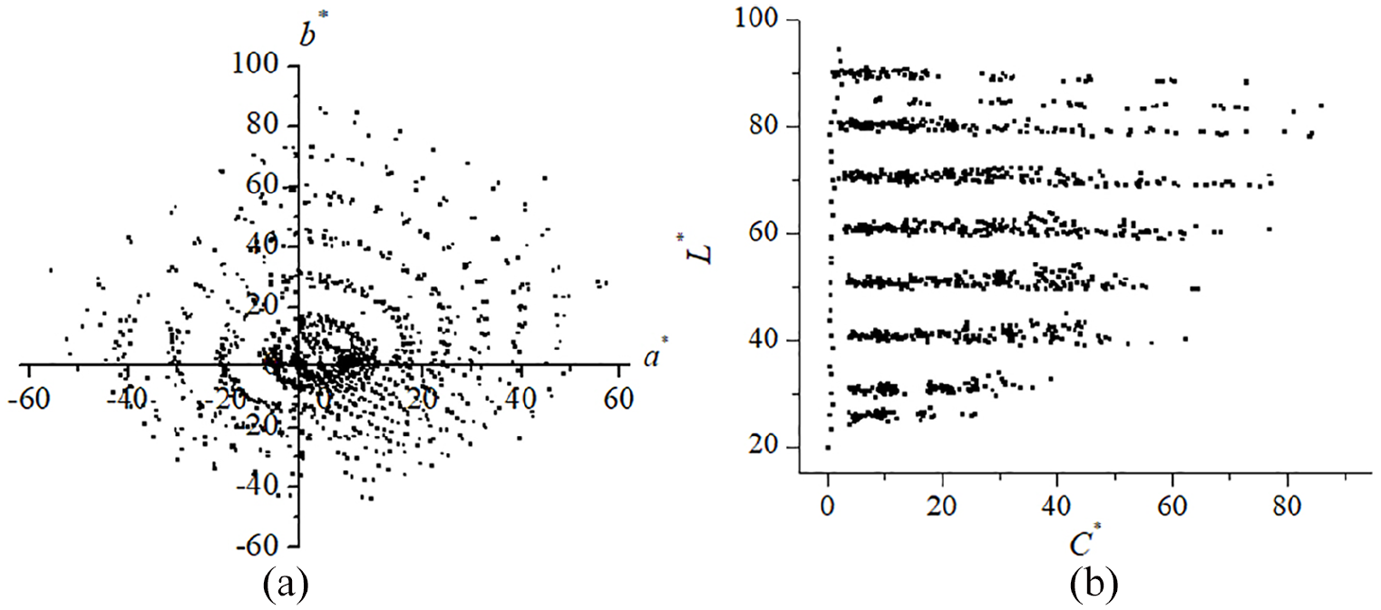
Chromatic coordinates (a) (a*, b*) and (b) (C*, L*) of the 1301 chips from the Munsell Color Book.

Figure 3.

A picture of Hue 5YR in the Munsell Color Book. ¹⁷

Measurement of samples

The 1301 color chips were measured to obtain their reflectance spectrum by utilizing a Cary 5000 UV-VIS-NIR spectrophotometer over the range of 360–830 nm at 1-nm-interval with 1-nm bandwidth at room temperature. The diffuse reflectance accessory this instrument used is internal DRA 2500.

Selection of basic parameters

Standard illuminant D₆₅ recommended by CIE and used most widely for textiles are selected, and its relative spectral power distribution S(λ) data in the range of 360–830 nm are available at 1-nm intervals. ¹⁸ Their S(λ)₁₀ at 10-nm intervals are extracted from the standard 1-nm S(λ) correspondingly.

CIE 1964 standard observer (10 degree) widely accepted in industrial practice is employed, and the color-matching functions $\overline{x}(\lambda )$ , $\overline{y}(\lambda )$ , and $\overline{z}(\lambda )$ at 1-nm intervals in band of 360–830 nm are obtained from CIE. ¹⁹ The data of 10-nm interval’s $\overline{x}{(\lambda )}_{10}$ , $\overline{y}{\left(\lambda \right)}_{10}$ , and $\overline{z}{(\lambda )}_{10}$ are extracted from the standard 1-nm $\overline{x}(\lambda )$ , $\overline{y}(\lambda )$ , and $\overline{z}(\lambda )$ . In order to simplify the expression, the subscript 10 conventionally used for the 10 degree observer is omitted, and 10 after (λ) represents the wavelength intervals of 10 nm.

Evaluation methods

The standard TSVs are computed by the standard algorithm recommended by CIE, and the TSVs obtained by other kinds of algorithms are taken as the test. This article compares the color difference between the standard’s and the test’s TSVs in order to evaluate the accuracy of the various methods.

With respect to the color difference formulas, in 1976, CIE officially recommended the CIELAB color difference formula; ²⁰ since it is not as uniform as expected, a series of improved formulas have been proposed basing on CIELAB. Among them, CMC_(l:c) is mostly used in textile and CIEDE2000^21,22 is the latest CIE standard. Both CMC_(l:c) and CIEDE2000_(2:1:1) are small color difference formulas for calculating the difference of 0–5 CIELAB units, ⁵ which coincide with the color differences obtained by various algorithms in this study. Therefore, besides CIELAB, CMC_(2:1) and CIEDE2000_(2:1:1) are also utilized in this article. The coefficients in CMC_(2:1) and CIEDE2000_(2:1:1) formulas are set as 2:1 and 2:1:1 which are used in textiles for acceptable evaluation.^23,24 The smaller the color difference, the better the accuracy of the method. For each method, total 3903(1301 samples × 3 color difference formulas) color difference values are calculated.

In the following part, Average represents the arithmetic mean. Median, means half of the total values are less (or greater) than. 80 percentile, means 80 percent of the total values are less than, so does the 95 percentile. Numbers in parentheses are the ranks for each statistical measure, which are summed in the last column. The statistics are based on an analysis of color differences. The smaller the rank sum is, the better the method performs.

Calculation, results, and discussion

All calculations in this article are sketched in Figure 4.

Figure 4.

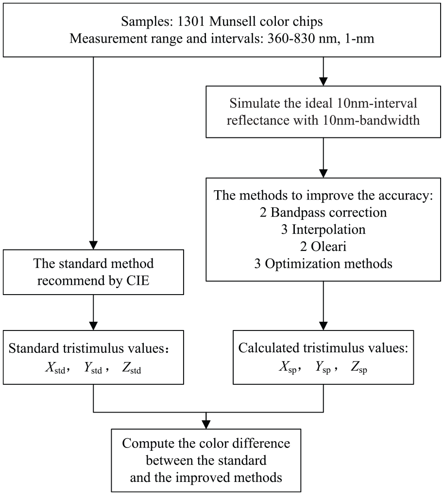
Flowchart of calculation process for improving the accuracy of TSVs.

Calculation of standard TSVs

Use the 1-nm interval’s S(λ), $\overline{x}(\lambda )$ , $\overline{y}(\lambda )$ , $\overline{z}(\lambda )$ , and reflectance R(λ) in the full range of 360–830 nm of 1301 samples to compute the standard TSVs XYZ_std according to equation (2) recommended by CIE.

Calculation of reflectance with bandpass in 10-nm intervals

During the reflectance measurement, the precision of the instrument is determined by the random error. ²⁵ Reflectance measured twice also shows difference even operated at the same position of the same sample. Hence, in practice, the instrument cannot output 1-nm interval data with 1-nm bandwidth as well as ∆λ nm intervals data with ∆λ nm bandwidth without an error. Besides, early research^12,13 showed that the measurement intervals should equal to the bandwidth in order to keep the result more accuracy. Therefore, in this article, equation (3) is used to generate the ideal 10-nm interval reflectance $\tilde{R}{(\lambda )}_{10}$ with 10-nm bandwidth.

Bandpass corrections

In order to compare the effects of the bandpass correction methods, the direct selection method (no bandpass correction), SS correction, and Fairman correction are calculated separately.

• Step 1: Use the method in section “Calculation of reflectance with bandpass in 10-nm intervals” to generate the ideal 10-nm intervals $\tilde{R}{(\lambda )}_{10}$ and then combine 10-nm S(λ)₁₀ and 10-nm $\overline{x}{(\lambda )}_{10}$ , $\overline{y}{(\lambda )}_{10}$ , and $\overline{z}{(\lambda )}_{10}$ to calculate the TSV XYZ_{_non} without bandpass correct.

• Step 2: Apply the SS bandpass correction method to 10-nm intervals $\tilde{R}{(\lambda )}_{10}$ , by equation (11), to compute the corrected reflectance ${\tilde{R}}_{\_SS}{(\lambda )}_{10}$ and together with the 10-nm S(λ)₁₀ and 10-nm $\overline{x}{(\lambda )}_{10}$ , $\overline{y}{(\lambda )}_{10}$ , and $\overline{z}{(\lambda )}_{10}$ to calculate XYZ_{_SS}.

• Step 3: Employ the Fairman bandpass correction method to 10-nm intervals $\tilde{R}{(\lambda )}_{10}$ , by equations (12)–(14), to compute the corrected reflectance ${\tilde{R}}_{\_F}{(\lambda )}_{10}$ and together with the 10-nm S(λ)₁₀ and 10-nm $\overline{x}{(\lambda )}_{10}$ , $\overline{y}{(\lambda )}_{10}$ , and $\overline{z}{(\lambda )}_{10}$ to calculate XYZ_{_F}.

• Step 4: Set XYZ_std calculated in section “Calculation of standard TSVs” as the standard and compute the color differences between XYZ_std and XYZ_{_non}, XYZ_{_SS}, and XYZ_{_F} in steps 1, 2, and 3.

Utilize MATLAB software to conduct programming, calculations, and statistical analysis. The results of two bandpass corrections and uncorrected data are listed in Table 1.

Table 1.

Color differences of non-correction and bandpass correction methods with standard method (numbers in parentheses are the ranks for each statistical measure).

Method	Formula	Median	Average	Max	80 percentile	95 percentile	Standard deviation	Rank sum
Without bandpass correction	CIELAB	0.0907(3)	0.1126(3)	0.5463(3)	0.1759(3)	0.2761(3)	0.0852(3)	18
	CMC(2:1)	0.0633(3)	0.0686(3)	0.2020(3)	0.0975(3)	0.1337(3)	0.0351(3)	18
	CIEDE2000	0.0559(3)	0.0595(3)	0.1781(3)	0.0831(3)	0.1119(3)	0.0293(3)	18
SS correction	CIELAB	0.0358(2)	0.0363(2)	0.1077(2)	0.0457(2)	0.0606(2)	0.0140(2)	12
	CMC(2:1)	0.0294(2)	0.0307(2)	0.0809(2)	0.0437(2)	0.0566(2)	0.0147(2)	12
	CIEDE2000	0.0238(2)	0.0249(2)	0.0611(2)	0.0366(2)	0.0443(2)	0.0117(2)	12
Fairman correction	CIELAB	0.0334(1)	0.0346(1)	0.1066(1)	0.0428(1)	0.0592(1)	0.0134(1)	6
	CMC(2:1)	0.0276(1)	0.0288(1)	0.0737(1)	0.0410(1)	0.0523(1)	0.0135(1)	6
	CIEDE2000	0.0223(1)	0.0234(1)	0.0591(1)	0.0343(1)	0.0417(1)	0.0109(1)	6

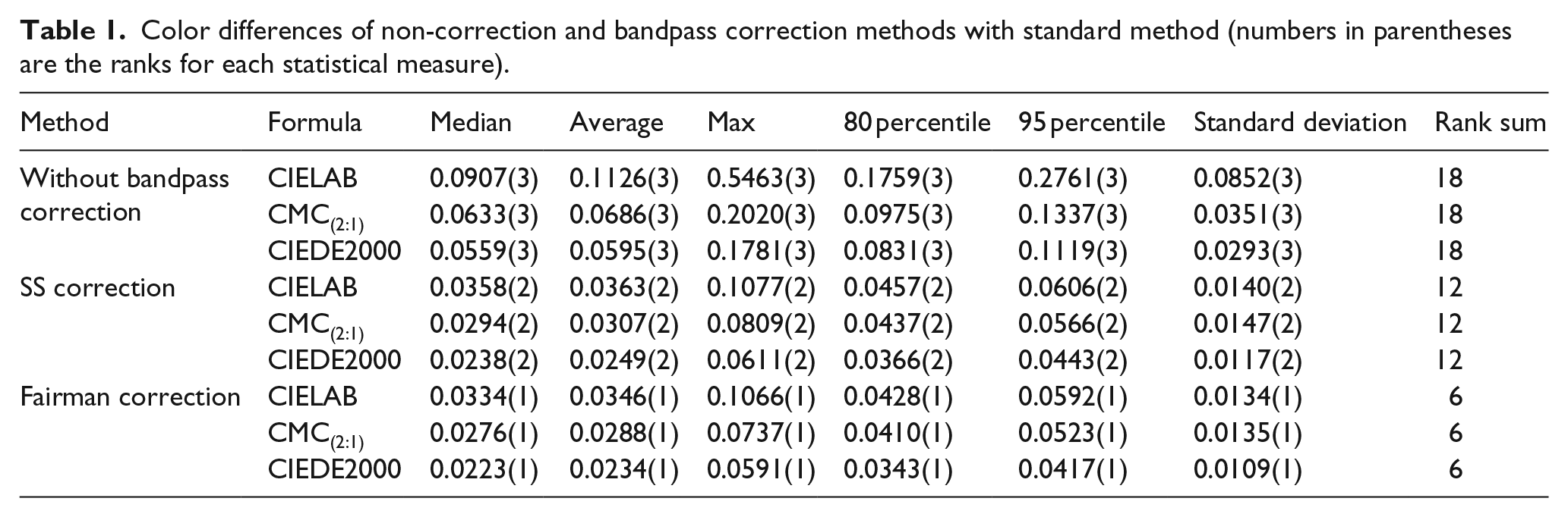
From Table 1, it is clear that bandpass correction methods have an obvious positive effect to reduce the color difference and increase the accuracy. The Fairman 5-point correction is just a little better than the SS 3-point correction. The color differences of the Fairman correction (median: 0.0334, 0.0276, 0.0223) is about 44% of the uncorrected processing (median: 0.0907, 0.0633, 0.0559).

Interpolation methods

• Step 1: Apply the three interpolation methods (Lagrange, Spline, and Sprague) to make the 10-nm ${\tilde{R}}_{\_SS}{(\lambda )}_{10}$ (gained in section “Bandpass corrections” step 2) into 1-nm ${\tilde{R}}_{\_SS\_Langrange}(\lambda )$ , ${\tilde{R}}_{\_SS\_Spline}(\lambda )$ , and ${\tilde{R}}_{\_SS\_Sprague}(\lambda )$ , calculate XYZ_{SS_Lagrange}, XYZ_{SS_Spline}, and XYZ_{SS_Sprague} with 1-nm $S(\lambda )$ , $\overline{x}(\lambda )$ , $\overline{y}(\lambda )$ , and $\overline{z}(\lambda )$ .

• Step 2: Apply the three interpolation methods (Lagrange, Spline, and Sprague) to make the 10-nm ${\tilde{R}}_{\_F}{(\lambda )}_{10}$ (obtained in section “Bandpass corrections” step 3) into 1-nm R_{F_Lagrange}(λ), R_{F_Spline}(λ), and R_{F_Sprague}(λ), calculate XYZ_{F_Lagrange}, XYZ_{F_Spline}, and XYZ_{F_Sprague} with 1-nm $S(\lambda )$ , $\overline{x}(\lambda )$ , $\overline{y}(\lambda )$ , and $\overline{z}(\lambda )$ .

• Step 3: Calculate color differences of the TSVs in step 1 and 2 with the standard XYZ_std.

The results are exhibited in Table 2 and will be analyzed with the Oleari methods together.

Table 2.

Color differences of three interpolation methods and Oleari methods under two bandpass correction methods.

Method	Formula	Median	Average	Max	80 percentile	95 percentile	Standard deviation	Rank sum
SS_Lagrange	CIELAB	0.0055(7)	0.0059(6)	0.0243(6)	0.0084(6)	0.0125(6)	0.0036(7)	38
	CMC(2:1)	0.0040(7)	0.0045(7)	0.0133(6)	0.0068(7)	0.0090(7)	0.0025(7)	41
	CIEDE2000	0.0034(7)	0.0038(7)	0.0129(8)	0.0056(7)	0.0077(7)	0.0021(7)	43
SS_Spline	CIELAB	0.0028(1)	0.0030(1)	0.0106(2)	0.0042(1)	0.0058(2)	0.0017(1)	8
	CMC(2:1)	0.0021(1)	0.0023(2)	0.0073(1)	0.0036(3)	0.0049(3)	0.0014(3)	13
	CIEDE2000	0.0017(1)	0.0019(1)	0.0057(3)	0.0030(3)	0.0040(3)	0.0011(3)	14
SS_Sprague	CIELAB	0.0029(2)	0.0030(1)	0.0099(1)	0.0044(2)	0.0057(1)	0.0017(1)	8
	CMC(2:1)	0.0021(1)	0.0024(4)	0.0078(4)	0.0037(4)	0.0052(4)	0.0015(4)	21
	CIEDE2000	0.0018(2)	0.0020(3)	0.0056(2)	0.0031(4)	0.0041(4)	0.0012(4)	19
F_Lagrange	CIELAB	0.0050(6)	0.0061(7)	0.0283(8)	0.0089(7)	0.0148(8)	0.0044(8)	44
	CMC(2:1)	0.0037(6)	0.0041(6)	0.0133(6)	0.0057(6)	0.0077(6)	0.0021(5)	35
	CIEDE2000	0.0032(6)	0.0035(6)	0.0124(6)	0.0049(6)	0.0068(6)	0.0018(6)	36
F_Spline	CIELAB	0.0030(3)	0.0037(4)	0.0172(4)	0.0056(5)	0.0087(5)	0.0027(5)	26
	CMC(2:1)	0.0021(1)	0.0023(2)	0.0077(3)	0.0032(2)	0.0046(2)	0.0012(2)	12
	CIEDE2000	0.0019(4)	0.0020(3)	0.0057(3)	0.0027(2)	0.0037(2)	0.0010(2)	16
F_Sprague	CIELAB	0.0030(3)	0.0035(3)	0.0162(3)	0.0055(4)	0.0084(4)	0.0026(4)	21
	CMC(2:1)	0.0021(1)	0.0022(1)	0.0075(2)	0.0031(1)	0.0044(1)	0.0011(1)	7
	CIEDE2000	0.0018(2)	0.0019(1)	0.0052(1)	0.0026(1)	0.0035(1)	0.0009(1)	7
SS_OWT0	CIELAB	0.0033(5)	0.0037(4)	0.0200(5)	0.0050(3)	0.0079(3)	0.0023(3)	23
	CMC(2:1)	0.0027(5)	0.0031(5)	0.0123(5)	0.0046(5)	0.0071(5)	0.0021(5)	30
	CIEDE2000	0.0024(5)	0.0026(5)	0.0105(5)	0.0037(5)	0.0056(5)	0.0016(5)	30
F_OWT0	CIELAB	0.0058(8)	0.0063(8)	0.0249(7)	0.0092(8)	0.0125(6)	0.0035(6)	43
	CMC(2:1)	0.0053(8)	0.0053(8)	0.0166(8)	0.0077(8)	0.0107(8)	0.0031(8)	48
	CIEDE2000	0.0044(8)	0.0044(8)	0.0124(6)	0.0061(8)	0.0086(8)	0.0024(8)	46
OWT2	CIELAB	0.0087(9)	0.0099(9)	0.0444(9)	0.0138(9)	0.0221(9)	0.0065(9)	54
	CMC(2:1)	0.0066(9)	0.0073(9)	0.0245(9)	0.0106(9)	0.0144(9)	0.0039(9)	54
	CIEDE2000	0.0058(9)	0.0062(9)	0.0233(9)	0.0087(9)	0.0121(9)	0.0033(9)	54

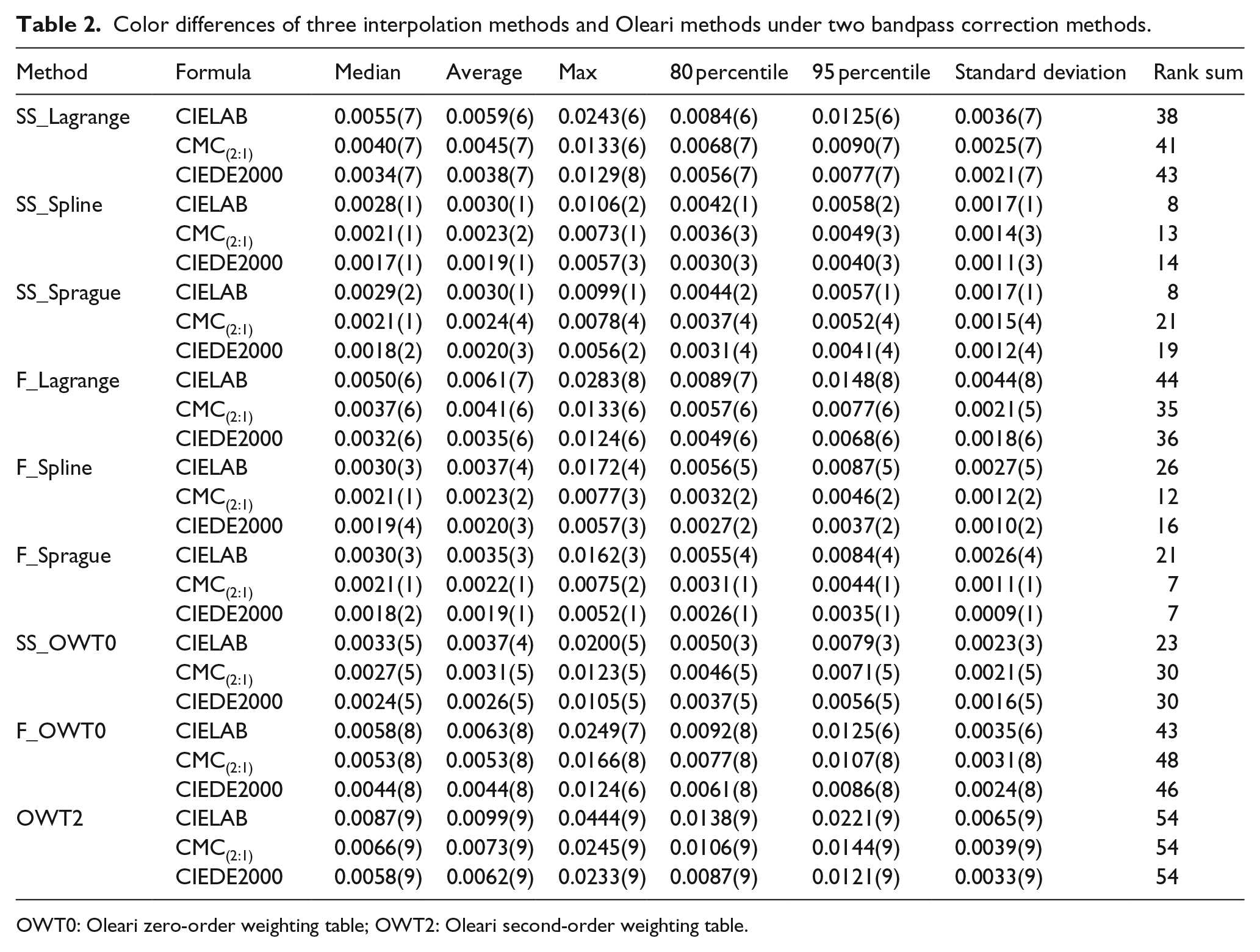
OWT0: Oleari zero-order weighting table; OWT2: Oleari second-order weighting table.

Oleari methods

• Step 1: Calculate the Table OWT0 and OWT2 with illuminant D₆₅ and 1964 observer according to the algorithm proposed by Oleari ⁷ and Li et al. ¹⁵

• Step 2: Calculate XYZ_{ss_OWT0}, XYZ_{F_OWT0} with the bandpass-corrected ${\tilde{R}}_{\_SS}{(\lambda )}_{10}$ , ${\tilde{R}}_{\_F}{(\lambda )}_{10}$ , and Table OWT0. Calculate XYZ_{_OWT2} with the non-bandpass-corrected $\tilde{R}{(\lambda )}_{10}$ and Table OWT2.

• Step 3: Calculate color differences of the TSVs XYZ_{ss_OWT0}, XYZ_{F_OWT0}, and XYZ__OWT2 in step 2 with the standard XYZ_std. The results are displayed in Table 2.

According to Table 2, at uniform 10-nm intervals, among the two bandpass correction methods combined with the three interpolation methods and Oleari methods, the rank is SS_Spline = F_Sprague > SS_Sprague > F_Spline > SS_OWT0 > F_Lagrange > SS_Lagrange > F_OWT0 > OWT2. The result in Table 1 shows that Fairman is a little better than SS correction, but the effect of Fairman and SS cannot be separately judged in Table 2. This may indicate that bandpass correction and interpolation show a combined effect, so SS correction plus Spline interpolation and Fairman correction plus Sprague interpolation perform the same, better than the others. Their color differences (median: 0.0028/0.0030, 0.0021/0.0021, 0.0017/0.0018) are less than 3% of the uncorrected uninterpolated method (median: 0.0907, 0.0633, 0.0559), improving the accuracy of TSVs greatly.

Optimization weighting table methods

• Step 1: Find ASTM E308 Table 6 with the condition of D₆₅ and CIE 1964 observers and compute XYZ_T6 with the 10-nm $\tilde{R}{(\lambda )}_{10}$ .

• Step 2: Apply the method introduced in the literature of Li et al. to derive Table LLR and Table LWL and calculate XYZ_LLR and XYZ_LWL with the 10-nm $\tilde{R}{(\lambda )}_{10}$ .

• Step 3: Calculate the color differences of the above TSVs XYZ_T6, XYZ_LLR, and XYZ_LWL with the standard XYZ_std.

ASTM gives Table 6 only in the range of 360–780 nm. In order to make comparison under the same condition, Table LLR and Table LWL are also utilized in the same range.

From Table 3, we can see that Table LWL is significantly better than Table 6 and Table LLR. Comparing the data in Tables 2 and 3, Table LWL still yields the best improvement on accuracy with color difference (median: 0.0007, 0.0005, 0.0004) approximate zero and only 7‰ of uncorrected and uninterpolated data (median: 0.0907, 0.0633, 0.0559).

Table 3.

Color differences of different optimization weighting table methods.

Method	Formula	Median	Average	Max	80 percentile	95 percentile	Standard deviation	Rank sum
Table 6	CIELAB	0.0053(3)	0.0053(3)	0.0115(3)	0.0066(3)	0.0075(3)	0.0015(2)	17
	CMC(2:1)	0.0042(3)	0.0046(3)	0.0139(3)	0.0062(3)	0.0086(3)	0.0021(3)	18
	CIEDE2000	0.0039(3)	0.0043(3)	0.0100(3)	0.0059(3)	0.0082(3)	0.0019(3)	18
Table LLR	CIELAB	0.0021(2)	0.0024(2)	0.0099(2)	0.0035(2)	0.0053(2)	0.0015(2)	12
	CMC(2:1)	0.0015(2)	0.0017(2)	0.0049(2)	0.0025(2)	0.0031(2)	0.0009(2)	12
	CIEDE2000	0.0013(2)	0.0013(2)	0.0031(2)	0.0020(2)	0.0025(2)	0.0006(2)	12
Table LWL	CIELAB	0.0007(1)	0.0007(1)	0.0031(1)	0.0009(1)	0.0012(1)	0.0003(1)	6
	CMC(2:1)	0.0005(1)	0.0005(1)	0.0024(1)	0.0008(1)	0.0012(1)	0.0003(1)	6
	CIEDE2000	0.0004(1)	0.0004(1)	0.0018(1)	0.0007(1)	0.0009(1)	0.0002(1)	6

Discussions

This article studies 14 algorithms of five types to improve the computation accuracy of CIE TSVs measured by the spectrophotometer, and they are summarized in Table 4.

Table 4.

14 algorithms in five types studied in this article.

Categories	Method	Function	Number of algorithms
M1	Bandpass correction	Reduces bandpass error	2
M2	Bandpass correction + interpolation	Reduces bandpass and intervals error	2×3 = 6
M3	Bandpass correction + Oleari zero-order weighting table	Reduces bandpass and intervals error	2×1 = 2
M4	Oleari second-order weighting table	Solving both bandpass and intervals error	1
M5	Optimization weighting table	Solving both bandpass and intervals error	3

Among the five types of methods, M4 and M5 can provide a weighting table at any intervals, any illuminants, and any colorimetric observers. So, the TSVs can be directly computed with the measured reflectance values. M1, M2, and M3 are a little bit more complicated because they had to deal with reflectance.

To make comparison, all the methods with their median color differences are drawn into Figure 5. From Figure 5 and Tables 1–3, the following results are concluded:

1. All the 14 algorithms yield very positive effects.

2. For the bandpass correction methods in M1, the Fairman correction is better than SS correction, and its median color difference is 44% of the unsolved data.

3. For the interpolation and Oleari methods in M2, M3, and M4, Spline interpolation based on SS bandpass correction is the best; its median color difference is about 3% of the unsolved data. Sprague interpolation under Fairman bandpass correction yield very close result to it.

4. For the optimization method in M5, Table LWL has the highest accuracy, and the median color difference drops to only 7‰ of unsolved data.

Figure 5.

Median color differences of different algorithms (10-nm intervals).

Among all the 14 algorithms above, the top 6 algorithms in view of improving accuracy are the following: Table LWL > Table LLR > SS_Spline > F_Sprague > SS_Sprague > Table 6. Further compare on the top six preferable methods, the calculation of the SS_Spline, F_Sprague, and SS_Sprague method is not as convenient as the weighting table. The accuracy of Table 6 method is not bad, and this method is recommended by ASTM and adopted by some spectrophotometers. However, due to the loss of the calculation method and only weighting tables under certain conditions are provided, Table 6 method lacks expansibility. From the results of this study, Table LWL algorithm is undoubtedly the best choice in solving the bandpass and 10-nm wavelength intervals error under D₆₅ illuminant.

Conclusion

TSVs are basic parameters to calculate colorimetric parameters. At present, when measuring the same color sample by different spectrophotometers, one gets different TSVs because of both measurement error and calculation error; this may confuse the users. So, a unified and high-precision method to calculate TSVs is demanded to reduce the errors when used in color management and communication. By analyzing the errors caused by spectrophotometers, this article focuses on overcoming the shortage of measurement bandpass and intervals. For the normal spectral reflectance data which do not comply with CIE’s recommendation of 1-nm intervals, 14 algorithms in five types were investigated to improve the accuracy of CIE TSVs, including bandpass correction, bandpass correction plus interpolation, bandpass correction plus Oleari OWT0, Oleari OWT2, and optimization weighting table.

Through a systematic comparison of 14 algorithms, the top 6 algorithms in view of improving accuracy are the following: Table LWL > Table LLR > SS_Spline > F_Sprague > SS_Sprague > Table 6. From the respect of convenience, the three Table algorithms are superior to interpolation method. Table LWL and Table LLR also have wider applicability and expansibility than Table 6, since algorithm for achieving Table 6 has lost.

Integrate consideration from convenience and accuracy, Table LWL algorithm is undoubtedly the best choice, which reduces the color difference to only 7‰ of the untreated data. It means that Table LWL method provides a wonderful solution for the users, and they do not need to buy a new spectrophotometer or change firmware in order to get 1-nm interval’s reflectance for accurate TSVs, and instrument with 10-nm intervals can be directly used with the Table LWL method to replace the original algorithm to obtain a better precision.

All the above results are discussed under the condition of D₆₅ illuminant, CIE 1964 standard colorimetric observer, and 10-nm uniform measurement intervals. For other illuminants, other observer, other intervals, or even for fluorescence samples, further tests can be conducted.