Sage Journals: Discover world-class research

Abstract

In this research, a statistical classification algorithm based on sparse coding is presented to classify the defects on E-glass fiber fabrics adaptively. First, all images are preprocessed by being convolved with the MR8 filter banks to obtain the filter responses. For the filter response space of each type of image, we will learn a Class-specific dictionary, and all the Class-specific dictionaries are concatenated to form a complete dictionary. Then, the reconstructed contribution rate of each atom of the complete dictionary to the image filter response is counted to obtain two types of histogram features of each image. Finally, the improved sparse representation classification is used to classify test defect images based on the histogram features. The proposed adaptive classification method has achieved an average classification accuracy of 96.67% on the dataset collected onsite. The results validate the superiority of the proposed method to E-glass fiber fabrics.

Keywords

E-glass fiber fabrics sparse representation sparse representation classification histogram features

Introduction

Glass fiber is formed when thin strands of silica-based or other formulation glass are extruded into many fibers with small diameters suitable for textile processing.¹ The most common type of glass fiber used in fiberglass is E-glass; E-glass (“E” because of initial electrical application) is alkali free and is the first glass prescription used in continuous filament formation. It now composes most of the fiberglass production in the world. The E-glass fiber fabric is the basic material of the copper clad laminate (CCL), which is the basic material of the printed circuit board (PCB).² Any presence of fabric defects in the CCL causes change in the electronic properties that might cause failure to the PCB. Using remedies to repair these defects will increase the processing time and costs. Classifying E-Glass fiber fabric defects is crucial for detecting any undesired defects in the produced part and for avoiding corrective actions. Therefore, early defects classification is critical.³

In most cases, the quality inspection of fabrics is carried out by visual inspection performed by human inspectors on some appraisal equipment, which will lead to the subjective error of the human inspectors in the classification task, thereby reducing the fabric quality. In recent years, with the development of machine learning, various methods have been applied to the classification of fabric defects. Jing et al.⁴ have extracted the texture defect from the regular texture by the Gabor filters and classified defects using local binary patterns and Tamura method, which have a good performance for fabrics with obvious texture. Mottalib et al.⁵ focused on classifying fabric defects based on geometric features of defects, which leads to the problem of poor generality. Kang and Zhang⁶ have proposed to incorporate the idea of the integral image into the Elo-rating algorithm(IIER), so that various fabric defects can be quickly detected. The generality of the algorithm for the identification of various types of fabric defects was confirmed in the final experimental stage.

Recently, sparse representation has shown great capabilities in handling problems such as audio processing,⁷ data expression,⁸ column selection,⁹ emotion recognition,¹⁰ face recognition,¹¹,¹² image compression,¹³ image denoising,¹⁴ color image representation,¹⁵ image super-resolution,¹⁶ medical imaging,¹⁷ motion segmentation¹⁸ and data segmentation,¹⁹ image classification,²⁰ and texture analysis.²¹ In these models, an input testing image or signal is encoded as a sparse linear combination of dictionary or training sample. Although sparse representation has a good performance in applications where the primary target is to reconstruct original signals or images as accurately as possible, such as in image expression, denoising, and coding, it is not the final goal in classification tasks as discriminating signals or images is more important here.²²

There is a new type of skill that applies label information in computing coefficients or dictionary, which is called supervised dictionary learning and sparse representation (S-DLSR).²³ According to Gangeh et al.,²³ S-DLSR methods can be categorized based on the following six criteria. (1) Learning one dictionary per class. The learning method can be either K-means²¹ or metaface.²⁴ (2) Unsupervised dictionary learning (DL) followed by supervised pruning.²⁵,²⁶ (3) Joint dictionary and classifier learning.²⁷ In this method, the dictionary and the classifier parameters are learned in a combined optimization problem. (4) Embedding class labels into the learning of dictionary.²⁸,²⁹ (5) Embedding class labels into the learning of sparse coefficients. And (6) learning a histogram of dictionary atoms over signal or image constituents.²¹ Wright et al.¹¹ have proposed a general classification algorithm for face recognition based on sparse representation computed by l1-minimization. Xu et al.³⁰ have improved the method¹¹ using the mathematically tractable l2 regularization rather than the l1 regularization, for which almost has a closed-form solution. And it is pointed out in Gangeh et al.²³ that the main drawback of the method in Wright et al.¹¹ is that they may cause a very large dictionary, as the size of the joint dictionary grows linearly with the number of classes.

The texton-based method^31–33 is one of the original methods which compute the histogram of dictionary atoms (textons) to model a texture image based on patches extracted. In this method, first learn a dictionary and then construct the histogram features using the training images. Varma and Zisserman³² model the image textures by the frequency histogram of filter response cluster centers (textons). In this method, supervised k-means was used to acquire the cluster centers to construct the dictionary. To compute the textons histogram, each patch was represented by the closest atom in the dictionary. This is the possible maximum sparsity as each patch is represented by only one dictionary atom.²³ The method³⁴ computes the dictionary and the corresponding sparse coefficients over the feature extracted from an image, and the ultimate classification task is to classify the whole image, not the patches in the previous methods. Therefore, the method is suitable for fabric defect classification.

Inspired by above researches, a novel feature extraction and classifier design is developed for effective defect classification. Representative features are extracted from the defect image by computing a histogram of dictionary atoms, and the adaptive sparse representation classification (SRC) classifier is used to classify defect images. The rest of the article is organized as follows: section “Brief introduction of SRC” presents the SRC. Section “The developed classification method for E-glass fiber fabric defects” introduces in detail the classification algorithm of E-glass fiber fabric defects. Section “Experimental evaluation” conducts extensive experiments, and section “Conclusion” concludes the article.

Brief introduction of SRC

SRC is one of the original DL methods used for face recognition, in which all training images of class i are viewed as class-specific dictionary $A_{i}$ , and then getting the complete dictionary A which is the concatenation of all the class-specific dictionaries $A = [A_{1}, A_{2}, \dots, A_{N}]$ , where N is the class number of all samples.

The SRC method is primarily divided into two steps: sparse coding and classification.

Sparse coding. The unknown test sample y $(y \in R^{M * 1})$ can be sparsely represented by the nearest few atoms (training images) in the class-specific dictionaries $A_{i}$ via the following formula

{\hat{x}}_{i} = \arg \min_{x_{i}} {{‖ y - A_{i} x_{i} ‖}_{2}^{2} + γ {‖ x_{i} ‖}_{1}}

(1)

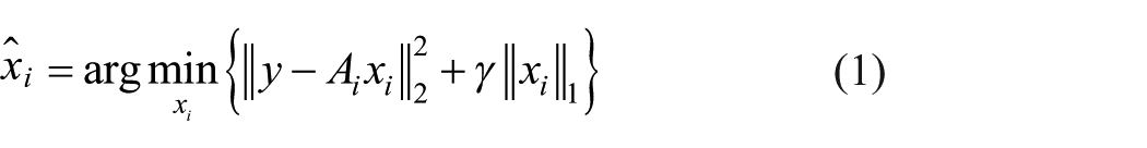
where $γ$ is a constant which is used to balance two terms in equation (1).

2. Classification. Sample y is then assigned to class i by minimizing the residual between y and its approximation

i d e n t i t y (y) = \arg \min e_{i} (y)

(2)

where $e_{i} (y) = {‖ y - A_{i} {\hat{x}}_{i} ‖}_{2}$ , $A = [A_{1}, A_{2}, \dots, A_{N}]$ , coefficient matrix $\hat{x}$ could be viewed as the concatenation of coefficient vectors $\hat{x} = [{\hat{x}}_{1}, {\hat{x}}_{2}, \dots, {\hat{x}}_{N}]$ , each of which corresponding to one class-specific dictionary.

The developed classification method for E-glass fiber fabric defects

In this section, we introduce the proposed defect classification method in detail. There are two major components in the proposed approach: image feature acquisition and classification.

Image feature acquisition

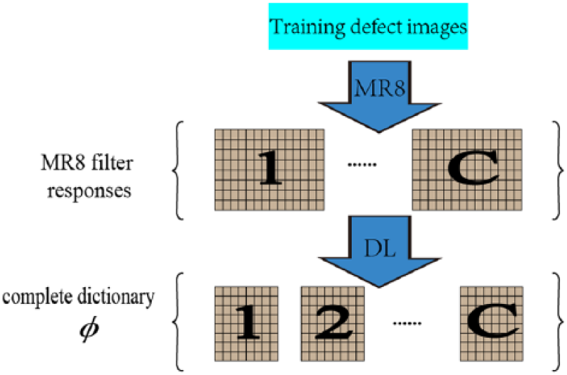
The picture collected from cooperative enterprise may be affected by various factors such as the intensity of light, the camera, or the surface of fabrics, and the image should be preprocessed first. All training images are convolved with the MR8 filter banks, and each image will acquire a filter response space where each filter response corresponds to a pixel which makes a large contribution to the defect image. Then, a complete dictionary was constructed by combining all class-specific dictionaries which were learned from filter responses of each defect. Finally, histogram features of each defect image are learned for complete dictionary atoms over filter response. This section mainly includes two parts: class-specific DL and the generation of histogram features.

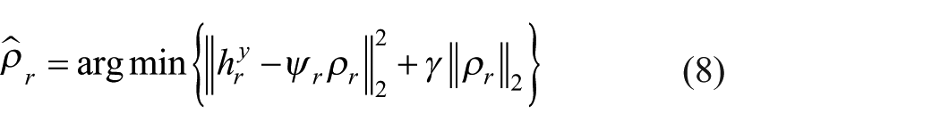
Class-specific DL. There are only six types of defects in the dataset, and we could learn a sub-dictionary per class (i.e. class-specific dictionary) without considering the problem of large dictionary size. Sparse representation is used to learn class-specific dictionary in our method. Assume there are C defects. C class-specific dictionaries for C defects can be learned, as shown in Figure 1. First, filter responses of each defect are clustered together, and an appropriate dimension reduction processing is performed to obtain a filter response matrix per class. And then the sparse representation of the matrix Y_i is used to learn a class-specific dictionary A_i for class i. The DL model is as follows

\min_{A_{i}, X_{i}} ({‖ Y_{i} - A_{i} X_{i} ‖}_{2}^{2} + λ {\sum_{i = 1}^{N} ‖ x_{i} ‖}_{1}) s . t . a_{j}^{T} a_{j} = 1

(3)

where $Y_{i} = [y_{i}^{1}, y_{i}^{2}, \dots, y_{i}^{N}] \in R^{M * N}$ represents filter response matrix for class i and N is the number of filter response. And $A_{i} = [a_{i}^{1}, a_{i}^{2}, \dots, a_{i}^{L}] \in R^{M * L}$ is the class-specific dictionary for class i and L is the number of dictionary atoms, and $X_{i} = [x_{i}^{1}, x_{i}^{2}, \dots, x_{i}^{N}] \in R^{L * N}$ is the coefficient matrix associated with dictionary A_i.

Figure 1.

Class-specific dictionary acquisition.

For the DL model, the solving process primarily includes sparse coefficient solution and dictionary updating. The sparse coefficient matrix X_i is obtained using the Matching Pursuit (MP) algorithm,³⁵ and the dictionary A_i is updated by the K-SVD algorithm³⁶ to obtain a new dictionary which can express the matrix Y_i better, the two processes are iterated until the iteration conditions are met to acquire the final class-specific dictionary.

2. Feature description. A class-specific dictionary can be learned for each defect using the DL model in the previous section, and all class-specific dictionaries are concatenated into a complete dictionary $ϕ = [A_{1}, A_{2}, \dots, A_{c}]$ . For each defect image, its defect can be mapped to the complete dictionary. Specifically, filter responses of each image can be denoted as $y = [y_{1}, y_{2}, \dots, y_{i}, \dots, y_{n}] \in R^{t * n}$ , where n is the number of filter response, and each filter response size is t*1. We refer to the filter response $y_{i}$ as the pixel feature vector. P atoms in the complete dictionary that are closest to the pixel feature vector $y_{i}$ are selected to constitute an adaptive dictionary $ϕ_{i}$ for sparse representation. The sparse representation (SR) model of the pixel feature vector $y_{i}$ is as follows

{\hat{θ}}_{i} = \arg \min_{θ_{i}} ({‖ y_{i} - ϕ_{i} θ_{i} ‖}_{2}^{2} + λ {‖ θ_{i} ‖}_{1})

(4)

where $ϕ_{i} = [a_{i}^{1}, a_{i}^{2}, \dots, a_{i}^{p}]$ , and $a_{i}^{p}$ denotes the Pth atom that is the closest to the vector $y_{i}$ . The corresponding coefficients $θ_{i} = [θ_{i}^{1}, θ_{i}^{2}, \dots, θ_{i}^{P}]^{T} \in R^{P * 1}$ are computed to obtain ${\hat{θ}}_{i}$ . The normalized coefficient $X_{i} = [x_{i}^{1}, x_{i}^{2}, \dots, x_{i}^{L * C}]$ over complete dictionary can be get, where L*C is the number of complete dictionary atoms. For each pixel feature y_i, most of the elements in the normalized coefficient X_i are zero, and the nonzero elements in X_i determine the atoms in the complete dictionary that contribute to the representation of the pixel feature y_i. All these coefficients are summed up for all pixel features of an image via the following function

h_{c} = \sum_{i = 1}^{n} X_{i}

(5)

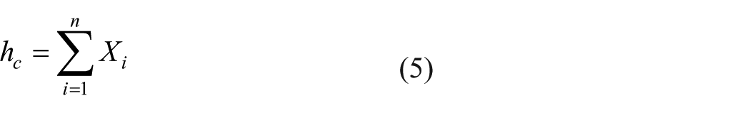
where n is the number of pixels that contribute significantly to the defect image, and the coefficient histogram $h_{c}$ of the defect image can be obtained. Since the original image cannot be approximated by the linear combination of dictionary atoms completely, there must be a residual. As such, the residual histogram h_r similar to the coefficient histogram is acquired from each image

h_{r} = \sum_{i = 1}^{n} e_{i}

(6)

where $e_{i} = [e_{i}^{1}, e_{i}^{2}, \dots, e_{i}^{j}, \dots, e_{i}^{L * C}]$ and $e_{i}^{j} = {‖ y_{i} - ϕ_{i}^{j} θ_{i}^{j} ‖}_{2},$ and n denotes the number of pixels that contribute significantly to the defect image.

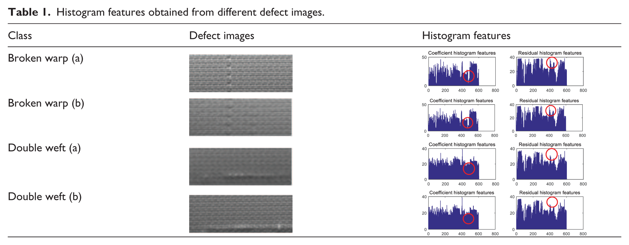
Two feature histograms of different class defect images are shown in Table 1. We can see that the two histogram features of the same defect images are almost the same; however, the two histogram features of the different defect images are obviously different. In addition, both class feature histograms also differ in the same defect image, which indicates that the two types of histogram features are complementary to the representation of fiberglass defects.

Table 1.

Histogram features obtained from different defect images.

Class	Defect images	Histogram features
Broken warp (a)
Broken warp (b)
Double weft (a)
Double weft (b)

Classification

Two histogram features h_c and h_r are extracted for all test images. In the SRC, replace all the images with histogram features of all images to complete the classification. In the method by Xu et al.,³⁰ the robustness and computational efficiency of the l₂ regularization-based representation method have been proved. We apply the l₂ regularization-based representation method to SRC. In detail, we assume that there are C defects and each defect has w defect images. Histogram features of ith class training sample are used to construct two kinds of class-specific dictionaries $ψ_{c}^{i} = [h_{c, 1}^{i}, h_{c, 2}^{i}, \dots, h_{c, w}^{i}], ψ_{r}^{i} = [h_{r, 1}^{i}, h_{r, 2}^{i}, \dots, h_{r, w}^{i}]$ , where $h_{c, j}^{i}, h_{r, j}^{i}$ denotes two histogram feature vectors of the jth image in the defect, then all class-specific dictionaries are concatenated into two complete dictionaries $ψ_{c}, ψ_{r}$ , where $ψ_{c} = [ψ_{c}^{1}, ψ_{c}^{2}, \dots, ψ_{c}^{C}]$ , $ψ_{r} = [ψ_{r}^{1}, ψ_{r}^{2}, \dots, ψ_{r}^{C}]$ . For a test image y, first its two histogram features $h_{c}^{y}, h_{r}^{y}$ are obtained and then are encoded by the histogram dictionary $ψ_{c}, ψ_{r}$

{\hat{ρ}}_{c} = \arg \min {{‖ h_{c}^{y} - ψ_{c} ρ_{c} ‖}_{2}^{2} + γ {‖ ρ_{c} ‖}_{2}}

(7)

{\hat{ρ}}_{r} = \arg \min {{‖ h_{r}^{y} - ψ_{r} ρ_{r} ‖}_{2}^{2} + γ {‖ ρ_{r} ‖}_{2}}

(8)

where $ρ_{c}$ , $ρ_{r}$ are the coefficient matrix associated with dictionary $ψ_{c}, ψ_{r}$ , respectively. The constraints of the sparse coefficients in model (7) (8) are both l2 norm, because it is easy to solve. Let the partial derivative of equations (7) and (8) with respect to ${\hat{ρ}}_{c}$ , ${\hat{ρ}}_{r}$ equal to 0, respectively, we have

{\hat{ρ}}_{c} = {(ψ_{c}^{T} ψ_{c})}^{- 1} ψ_{c}^{T} h_{c}^{y}

(9)

{\hat{ρ}}_{r} = {(ψ_{r}^{T} ψ_{r})}^{- 1} ψ_{r}^{T} h_{r}^{y}

(10)

Equations (9) and (10) can be written as: ${\hat{ρ}}_{c} = P_{c} * h_{c}^{y}$ , ${\hat{ρ}}_{r} = P_{r} * h_{r}^{y}$ where $P_{c} = {(ψ_{c}^{T} ψ_{c})}^{- 1} ψ_{c}^{T}$ ; $P_{r} = {(ψ_{r}^{T} ψ_{r})}^{- 1} ψ_{r}^{T}$ can be pre-calculated as two projection matrices, then the reconstruction error of the test image histogram feature over the ith class-specific dictionary is calculated as

e r r_{c}^{i} = {‖ h_{c}^{y} - ψ_{c}^{i} {\hat{ρ}}_{c}^{i} ‖}_{2}

(11)

e r r_{r}^{i} = {‖ h_{r}^{y} - ψ_{r}^{i} {\hat{ρ}}_{r}^{i} ‖}_{2}

(12)

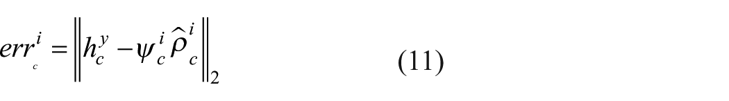
Apply equations (11) and (12) to calculating two reconstruction errors of the histogram feature of the test image y over each class-specific dictionary

E r r_{c} = [e r r_{c}^{1}, e r r_{c}^{2}, \dots, e r r_{c}^{i}, \dots, e r r_{c}^{C}]

(13)

E r r_{r} = [e r r_{r}^{1}, e r r_{r}^{2}, \dots, e r r_{r}^{i}, \dots, e r r_{r}^{C}]

(14)

We have found that both histogram features are discriminative and complementary to the image defects from Table 1, therefore the test image y will be classified by the weighting average method

E r r_{f} = ω \cdot E r r_{c} + (1 - ω) \cdot E r r_{r}

0 \leq ω \leq 1

(15)

where $ω$ is the weight and the image y is classified by the following function

i d e n t i t y (y) = \arg \min E r r_{k} (y)

k = 1, 2, \dots, C

(16)

Experimental evaluation

There are few researches on the classification of E-glass fiber fabric defects. The main difficulty for defect classification is the lack of publicly available datasets. We tried to provide a dataset containing the major defects of E-glass fiber fabric in order to facilitate the development of future algorithms. To create the dataset, the ccd camera with 4k pixels is used to actually collect the defect image in the factory. There are four primary types of E-glass fiber fabric defects: edge, broken warp, double weft, and pilling. We conducted a practical investigation on the E-glass fiber fabric defects in the factory and found that the above four defects accounted for about 85% of all defects, and remaining defects were messy and difficult to distinguish. To enhance the effect of the experiment, the shading and defect-free (normal) on the fabric were also considered as two classes. Therefore, the image dataset includes six classes, as shown in Figure 2. In this experiment, there are 120 images for each defect and every image size is set to 220*80.

Figure 2.

Six class fiberglass fabric defect images: (a) edge, (b) broken warp, (c) double weft, (d) pilling, (e) shading, and (f) defect-free.

All experiments were conducted in a MATLAB R2014b environment on a desktop PC with a 3.2GHZ quad-core Intel processor and 8G memory. 30, 40, 50, 60, 70, 80, 90, 100, and 110 images are randomly selected to form the training dataset, and for each setting, the experiment was run 20 times and the average classification accuracy is recorded. At the stage of DL and sparse coding, the parameter λ in equations (3) and (4) are both set to 0.5. In the process of adaptive dictionary encoding, the adaptive dictionary atom number is set to 7 because the pixel feature vector is eight-dimensional.

In the process of classification, when 30-110 were used as training sample numbers for each defect, separately, the weight for two reconstruction errors were 0.05, 0.05, 0.05, 0.35, 0.85, 0.25, 0.25, 0.85, and 0.95.

Evaluation of the proposed method

In order to verify again that two types of histogram features are complementary for the expression of defect images, all errors, containing err_c, err_r, and err_f, are used to classify the test defect images. The classification results are shown in Figure 3. It can be seen from the figure that it is obviously much better to classify the test image by $e r r_{f} .$ Figure 4 shows some of the two most common misclassification examples.

Figure 3.

Different reconstruction error classification accuracy.

Figure 4.

For images (a) broken warp and (b) defect-free, due to the fact that the defects in the radial direction of the defect image are even hardly distinguished by the human eye, the two types of images are easily misclassified by the proposed method.

Comparison evaluation

The proposed method is first compared with the SRC method. The experiment draws the defect classification accuracy of the two methods by constantly changing the number of training samples. The classification results are shown in Figure 5. The experimental results show that the proposed method is more suitable for E-glass fiber fabric defects than the traditional SRC method, and it is verified that the dictionary obtained from the image histogram feature is better than the dictionary constructed directly from the training image.

Figure 5.

Classification accuracy of SRC and proposed method with different training samples.

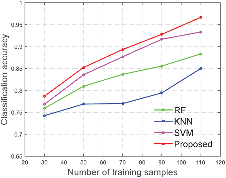
Then, we compare the proposed method with three popular classification methods: random forest (RF),³⁷ K-nearest neighbor (KNN),³⁸ and support vector machine (SVM).³⁹ As the number of training samples increases, the classification accuracy of each classification method will become higher. All classification methods adopt the histogram features proposed in the paper as image features. The classification accuracy of different classification methods with different training samples is shown in Figure 6. We can see that the proposed method has advantages over the popular classification methods in different training samples.

Figure 6.

Classification accuracy of different methods in different training samples.

The classification accuracy of all classification methods was listed in the table when the classification sample is 110, as shown in Table 2. Obviously, the application of the proposed method in the classification of E-glass fiber fabric defects shows a very good advantage.

Table 2.

Classification rates by different methods when the number of training samples is relatively large.

Method	Classification accuracy (%)
MR8 + RF	88.33
MR8 + KNN	85.00
MR8 + SVM	93.33
Proposed	96.67

RF: random forest; KNN: K-nearest neighbor; SVM: support vector machine.

In the actual factory, the classification speed for image defects is very important and has a serious impact on plant efficiency. We compared the average running time of above methods. All training samples used in the comparison experiment were 110 and the average running time is shown in Table 3. Although the proposed method is not the fastest, the proposed method is adaptable to the classification of E-glass fiber fabric defects due to its good classification accuracy.

Table 3.

The average running time for different classification methods when the training samples number is 110.

Method	Average running time (s)
MR8 + RF	0.2766
MR8 + KNN	0.0865
MR8 + SVM	0.4544
Proposed	0.1004

RF: random forest; KNN: K-nearest neighbor; SVM: support vector machine.

Conclusion

In this article, we have proposed an improved statistical classification method for the E-glass fiber fabric defects. The actual image is preprocessed by the MR8 filter bank to suppress the large changes that may appear in the image. And the sparse representation is applied to the histogram features acquisition, which enhance the ability of the histogram feature to characterize the defect image. In the classification stage, we have improved the SRC classifier using l₂ regularization-based representation method to achieve the classification of the defect image. The experimental results confirm the superiority of the proposed method. At the same time, in order to solve the problem of less available databases, three Basler line array cameras were used to image the fabric with a width of 1.8 m under the transmission of OPT’s line light source when the fabric inspection machine runs at 80 m/min. The camera model is raL4096-24gm with a 35 mm Nikon lens, and the camera is mounted at a height of 0.7 m and the corresponding width of a single camera is 0.574 m. A more consistent dataset was obtained under the device. In future work, we will study how to use a smaller number of training samples to achieve high classification accuracy.

Footnotes

Declaration of conflicting interests

The author(s) declared no potential conflicts of interest with respect to the research, authorship, and/or publication of this article.

Funding

The author(s) received no financial support for the research, authorship, and/or publication of this article.

References

Zhang

Matinlinna

JP.

E-glass fiber reinforced composites in dental applications. Silicon 2012; 4(1): 73–78.

Wang

Chen

Zheng

et al . Study on the filament yarns spreading techniques and assessment methods of the electronic fiberglass fabric. IOP Conf Ser-Mat Sci 2018; 322(2): 22–37.

Gaja

Liou

Defect classification of laser metal deposition using logistic regression and artificial neural networks for pattern recognition. Int J Adv Manuf Tech 2018; 94(1–4): 315–326.

Jing

Zhang

Wang

et al . Fabric defect detection using Gabor filters and defect classification based on LBP and Tamura method. J Text I 2013; 104(1): 18–27.

Mottalib

Rokonuzzaman

Habib

et al . Fabric defect classification with geometric features using Bayesian classifier. In: Proceedings of the international conference on advances in electrical engineering (ICAEE), Dhaka, Bangladesh, 17–19 December 2015, pp. 137–140. New York: IEEE.

Kang

Zhang

A universal defect detection approach for various types of fabrics based on the Elo-rating algorithm of the integral image. Textile Research Journal 2019. doi: 10.1177/0040517519840636.

Chan

TST

Yang

. Informed group-sparse representation for singing voice separation. IEEE Signal Proc Let 2017; 24(2): 156–160.

Elhamifar

Sapiro

Vidal

See all by looking at a few: sparse modeling for finding representative objects. Proc CVPR IEEE 2012; 157: 1600–1607.

Farahat

Elgohary

Ghodsi

et al . Distributed column subset selection on MapReduce. In: Proceedings of the international conference on data mining (ICDM), Dallas, TX, 7–10 December 2013, pp. 171–180. New York: IEEE.

10.

Gangeh

Fewzee

Ghodsi

et al . Multiview supervised dictionary learning in speech emotion recognition. IEEE-ACM T Audio Spe 2014; 22(6): 1056–1068.

11.

Wright

Yang

Ganesh

et al . Robust face recognition via sparse representation. IEEE T Pattern Anal 2009; 31(2): 210–227.

12.

Yang

Zhang

Feng

et al . Fisher discrimination dictionary learning for sparse representation. IEEE I Conf Comp Vis 2011; 24(4): 543–550.

13.

Neethu

Jabbar

Improved quality of JPEG compressed image using approximate K-SVD algorithm. In: Proceedings of the international conference on innovations in information, embedded and communication systems (ICIIECS), Coimbatore, India, 19–20 March 2015, pp. 1–6. New York: IEEE.

14.

Elad

Aharon

Image denoising via sparse and redundant representations over learned dictionaries. IEEE T Image Process 2006; 15(12): 3736–3745.

15.

et al . Vector sparse representation of color image using quaternion matrix analysis. IEEE T Image Process 2015; 24(4): 1315–1329.

16.

Yang

Wright

Huang

et al . Image super-resolution via sparse representation. IEEE T Image Process 2010; 19(11): 2861–2873.

17.

Gangeh

Sørensen

Shaker

et al . A texton-based approach for the classification of lung parenchyma in CT images. Med Image Comput Comput Assist Interv 2010; 13: 595–602.

18.

Rao

Tron

Vidal

et al . Motion segmentation via robust subspace separation in the presence of outlying, incomplete, or corrupted trajectories. In: Proceedings of the conference on computer vision and pattern recognition (CVPR), Anchorage, AK, 23–28 June 2008, pp. 1–8. New York: IEEE.

19.

Elhamifar

Vidal

Sparse subspace clustering: algorithm, theory, and applications. IEEE T Pattern Anal 2013; 35(11): 2765–2781.

20.

Wang

Yang

et al . Locality-constrained linear coding for image classification. Proc CVPR IEEE 2010; 119: 3360–3367.

21.

Gangeh

Ghodsi

Kamel

MS.

Dictionary learning in texture classification. Int Conf Image Anal Recognit 2011; 6753: 335–343.

22.

Huang

Aviyente

Sparse representation for signal classification. ADV Neur In 2007; 19: 609–616.

23.

Gangeh

Farahat

Ghodsi

et al . Supervised dictionary learning and sparse representation—a review. Comp Sci 2015; 2: 1–56.

24.

Yang

Zhang

Yang

et al . Metaface learning for sparse representation based face recognition. IEEE Image Proc 2010; 119: 1601–1604.

25.

Fulkerson

Vedaldi

Soatto

Localizing objects with smart dictionaries. Eur Conf Comp Vis 2008; 5302: 179–192.

26.

Winn

Criminisi

Minka

Object categorization by learned universal visual dictionary. IEEE I Conf Comp Vis 2005; 2: 1800–1807.

27.

Zhang

Discriminative K-SVD for dictionary learning in face recognition. Proc CVPR IEEE 2010; 119: 2691–2698.

28.

Zhang

Huang

TS.

Simultaneous discriminative projection and dictionary learning for sparse representation based classification. Pattern Recogn 2013; 46(1): 346–354.

29.

Lazebnik

Raginsky

Supervised learning of quantizer codebooks by information loss minimization. IEEE T Pattern Anal 2009; 31(7): 1294–1309.

30.

Zhong

Yang

et al . A new discriminative sparse representation method for robust face recognition via 12 regularization. IEEE T Neur Net Lear 2017; 28(10): 2233–2242.

31.

Varma

Zisserman

A statistical approach to texture classification from single images. INT J Comput Vision 2005; 62(1–2): 61–81.

32.

Varma

Zisserman

A statistical approach to material classification using image patch exemplars. IEEE T Pattern Anal 2009; 31(11): 2032–2047.

33.

Julesz

Textons, the elements of texture perception, and their interactions. Nature 1981; 290(5802): 91–97.

34.

Xie

Zhang

You

et al . Effective texture classification by texton encoding induced statistical features. Pattern Recogn 2015; 48(2): 447–457.

35.

Chardon

Necciari

Balazs

Perceptual matching pursuit with Gabor dictionaries and time-frequency masking. In: Proceedings of the international conference on acoustics, speech and signal processing (ICASSP), Florence, 4–9 May 2014, pp. 3102–3106. New York: IEEE.

36.

Rubinstein

Peleg

Elad

Analysis K-SVD: a dictionary-learning algorithm for the analysis sparse model. IEEE T Signal Proces 2013; 61(3): 661–677.

37.

Breiman

Random forests. Mach Learn 2001; 45(1): 5–32.

38.

Wang

KNN classification algorithm for multiple statuses detection of through-wall human being. In: Proceedings of the international conference in communications, signal processing, and systems (CSPS), Chongqing, China, 21–22 October 2016, pp.229–235. New York: Springer

39.

Demirhan

Salor

. Classification of targets in SAR images using SVM and k-NN techniques. In: Proceedings of the signal processing and communication application conference (SIU), Zonguldak, Turkey, 16–19 May 2016, pp. 1581–1584. New York: IEEE.

Statistical classification for E-glass fiber fabric defects based on sparse coding

Abstract

Keywords

Introduction

Brief introduction of SRC

The developed classification method for E-glass fiber fabric defects

Image feature acquisition

Classification

Experimental evaluation

Evaluation of the proposed method

Comparison evaluation

Conclusion

Footnotes

Declaration of conflicting interests

Funding

References