Sage Journals: Discover world-class research

Abstract

We studied the algorithms of button defect detection, while metal button defect detection is seldom explored in the literature. In this paper, we propose to effectively improve the detecting speed, accuracy, and robustness of the model. We propose a new method of cascading Extreme Learning Machine (ELM) and Sparse Representation Classification (SRC). This method transforms the defect detection problem into a pattern classification problem. First, we preprocess the input button images via eliminating reflection, edges extraction, and dimensionality reduction. ELM has a faster learning speed and better detecting accuracy than the single layer perceptron and support layer machine. ELM was utilized to estimate the probability of the defective buttons, with parameters obtained from the five-fold cross-validation method. SRC was used to reclassify those button images with high noise. Our method improved the detection accuracy, as well as guaranteed the detecting speed. We showed state-of-the-art performance in comparison to other approaches.

Keywords

Button Defect Detection Computer Vision Extreme Learning Machine Five-Fold Cross-Validation Sparse Representation Classification

Introduction

Buttons with various shapes and styles are widely-used in the modern clothing industry. To improve the quality of products, clothing industries and researchers have paid more attention to the techniques of button quality inspection.¹ In recent decades, image classification and machine vision have been widely utilized in defect detection, security systems, human-computer interaction, and other various applications.²

Recently, many algorithms have been developed for button defect detection. In 2015, Chen³ proposed an on-line defect detection method of button hole and color difference. In 2016, Zhou⁴ proposed an on-line monitoring algorithm to detect button character defects. In Zhou's paper, a grid method is used to extract features of button characters, and then buttons were classified by the Support Vector Machine (SVM).⁵ In 2018, Li⁶ proposed a method, using Gaussian filtering, edge detection, and threshold segmentation, to achieve the classification between positive and negative buttons. However, most methods are mainly about edge and inner hole defect detection of plastic buttons. Compared to plastic buttons, it is a more challenging task to detect metal button defects because metal buttons are smaller and sensitive to light.⁷

Compared to the traditional analytical modeling method, Extreme Learning Machine (ELM),^8,9 which is a single hidden layer network, has an efficient real-time processing speed. It initializes input weights and bias within a certain range randomly, optimizes the output weight matrix based on the least squares approximation, and calculates the generalized inverse of the data matrix. It has strong generalization and can be used in various applications including button defect detection. However, ELM is not robust enough for interference, such as high noise. Sparse Representation Classification (SRC)¹⁰ has excellent robustness, generalization ability, and anti-interference ability. It can transform the general signal classification problem into a sparse representation problem. A large number of experiments have proved that such classifier is insensitive to exceptional data, and the selected feature space can be well applied to image classification. Consequently, it is complementary to cascade ELM and SRC in terms of time efficiency and classification accuracy.¹¹ However, our method is different as follows.

Our regularization parameters are selected as the best ones by using the five-fold cross-validation method.

In the training stage of ELM, the number of hidden nodes is selected as the one corresponding to the optimal f1-score through experiments under the use of multiple parameters.

In the training stage of ELM, the number of input parameters is selected as the best one through multiple experiments under the dimensionality reduction of metal button images.

In this study, we present a network cascading ELM and SRC, named ELM-SRC, which combines the advantages of ELM and SRC. The regularization parameters of ELM are selected as the best ones by the five-fold cross-validation method, which is different from other methods using ELM. The first results of button classification are obtained by ELM, and then SRC was used to reclassify and obtain the final classification results by querying a complete dictionary of the sparsely represented. In the classification stage, button images are evaluated by Single Hidden Layer Feedforward Neural Networks (SLFNs). Tat is, the two outputs of ELM model represent the probability of the button quality. The larger difference between predicted probability of two different classes, the better the classification result. When the difference of two outputs’ probability is less than the predefined threshold, SRC can be used to reclassify those buttons as a validation for its excellent robustness and outstanding recognition ability. The final result of the classification was obtained by querying the complete dictionary of the SRC. The experimental results show that the proposed cascaded network had a more significant improvement than only using ELM.

Our contributions are the following:

We propose a method cascading Extreme Learning Machine and Sparse Representation Classification to detect metal buttons. It efficiently improves the detecting speed, accuracy, and robustness.

Five-folder cross validation is used to get the regularization parameters of ELM, which improves detection accuracy.

The misclassified samples are reclassified by using SRC, which further improves the accuracy of the model.

The rest of this paper is organized as follows. Collecting, labeling, and preprocessing of button images are introduced. The cascaded network ELM-SRC is described for metal button defect detection. The experimental procedure and results are given. Finally, the conclusion and future work are presented.

Image Preprocessing

In this section, a new preprocessing flow for metal buttons is proposed. The flow chart is shown in Fig. 1.

Fig. 1

Preprocessing flowchart.

Collecting Images

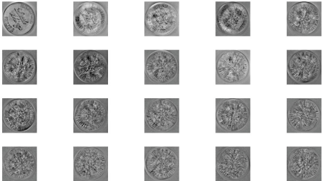
The dataset collected included 2000 positive and 1200 negative samples of metal buttons. Fig. 2 shows some samples of positive and negative buttons in the dataset. Positive samples are buttons with no problems. Negative samples are buttons with spots, scratches, pattern errors, and so forth.

Fig. 2

Samples of buttons. The left one is a positive sample, the middle one is a negative sample with a wrong pattern, and the right one is a negative sample with speckle on the surface.

Eliminating Reflection

Because the surface of the metal button is easily affected by the light, if the focal length and size of the aperture are not selected appropriately, it will cause a local area reflection problem that will often interfere with the subsequent detection of the defect.¹² Therefore, in the experiment, firstly, we set the camera to a small aperture, long distance, plus polarizer filter, and installed the camera holder in front of the lens to reduce the influence of reflection on the device. Secondly, we also took measures to eliminate reflection of collected images algorithmically. Here we use an iteratively updated template matching algorithm, an exemplar-based algorithm,¹² using pixel information in neighboring area of reflective points to update their pixel values. Thereby, this algorithm can reduce the interference of high-light noise on the subsequent detection.

On the button image, the highlight area is often caused by camera exposure and ambient light intensity, and these areas are close to saturation with large pixel values. We can calculate the difference between the RGB three-channel pixel values of a certain point of the image and a certain upper threshold at first. If the difference is equal to zero, the point is a reflection point. Therefore, a highlight region can be obtained. We will illustrate the idea of the exemplar-based algorithm with reference to Fig. 3.

Fig. 3

Algorithm for eliminating image reflection.

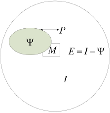
In Fig. 3, I represents image area, Ψ denotes the reflective area, E represents the normal area, P = ∂Ψ denotes the boundary of the reflective area, and M represents the local matrix neighborhood of a point on the boundary. The reflective area is filled from the outside to the inside by the exemplar-based algorithm, constantly reducing the reflective area. The algorithm selects the filling order of the reflective points according to the information contained in the rectangular regions, which corresponds to the different peripheral points. The amount of information is expressed by Eq. 1.

I n f o (p) = \frac{\sum_{q \in E \cap^{​} M} C (q)}{S (M)} • \frac{| \nabla I_{p}^{*} n_{p} |}{α}

(Eq. 1)

M and E are the rectangular area and non-reflective area respectively. C(q) is the sum of the pixel values that represent the intersection of M and E, S(M) is the area value of M, ∇I _p is the gradient at the pixel point p, n _p is the unit normal vector at the pixel point of P, and α is a regularization factor. The above formula indicates that the area of P is expected to contain as much information as possible so that the point is in a strong edge extension area, and the algorithm needs to preferentially fill the reflective part of the rectangular area corresponding to the point.

The point with the highest priority of Info(p) is denoted as $\hat{p}$ , and the corresponding local matrix neighbor region is M_p. Ten, the reflective region of M_p needs to be filled first, and the filling method uses Eq. 2.

{\hat{M}}_{p} = \arg \min_{M_{q}} d (M_{q}, M_{p})

(Eq. 2)

M _q ∊ E is a rectangular block in the known non-reflective area, d(M_q, M_p) is the sum of the squares of the difference between the pixel values of the corresponding points of the two area blocks, and the pixel value of the rectangular block M having the smallest distance is selected to fill the reflective part. The reflective area is reduced with each filling operation, and it iterates until all the reflective areas are filled. The comparison results before and after processing are shown in Fig. 4.

Fig. 4

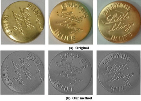
Comparison before and after processing. The first row are original images, the second row are processed images.

Edges Extraction and Dimensionality Reduction

After eliminating reflection, we convert button images to grayscale images, then sharpen them by the Laplace transform algorithm, and extract the edge information. Negative samples after transformation and corresponding original images are shown in Fig. 5. Because ELM is a relatively shallow network, too many dimensions will overfit the network. Therefore, we extract the principal components from the images using the Principal Component Analysis (PCA)¹³ algorithm. Here the 200-dimensional principal component vector is retained, which is visualized in Fig. 6. Finally, the 200-dimensional vector is normalized to obtain standard data.

Fig. 5

Comparison of negative samples and Laplace transform.

Fig. 6

The main component of buttons.

ELM-SRC Network Model

In this section, we introduce the ELM classifier, SRC classifier, and ELM cascading SRC classifier respectively. The latter is a new classification network architecture cascading sparse feature representation, which is applied to the secondary detection of button defects.

ELM Classifier

In ELM, the weights and biases are randomly initialized.14 The output layer is used as the decision layer of the classification, and its weights are obtained by solving the generalized inverse of the matrix.

Assuming the dataset in Eq. 3:

X = {(x_{j}, t_{j}) ∣ x_{j} \in R^{n}, t_{j} \in R^{m}}_{j = 1}^{N}

(Eq. 3)

Where x _i = [x_i₁, x_i₂,...x_im] ^T , t _i = [t _i ₁,t_i ₂,...t_in] ^T ,i =1,2...M, the expression of the ELM algorithm is shown in Eq. 4.¹⁵

\sum_{i = 1}^{L} β_{i} g_{i} (x_{j}) = \sum_{i = 1}^{L} β_{i} g_{i} (w_{i} x_{j} + b_{i}) = o_{j}

(Eq. 4)

w_i is the input weight, b_i is the bias (they are randomly initialized and fixed), and β_i is the output weight, which needs to be obtained by the model. ELM needs to solve the following convex programming problem shown in Eqs. 5–7.¹⁶

\min_{β} ∥ H β - T ∥_{F}

(Eq. 5)

\begin{matrix} H (w_{1}, \dots, w_{L}, b_{1}, \dots, b_{L}) \\ = [\begin{matrix} g (w_{1} x_{1} + b_{1}) & L & g (w_{L} x_{1} + b_{L}) \\ M & L & M \\ g (w_{1} x_{N} + b_{1}) & L & g (w_{L} x_{N} + b_{L}) \end{matrix}] \end{matrix}

(Eq. 6)

β = [\begin{matrix} β_{1}^{T} \\ M \\ β_{L}^{T} \end{matrix}], T = [\begin{matrix} t_{1}^{T} \\ M \\ t_{N}^{T} \end{matrix}]

(Eq. 7)

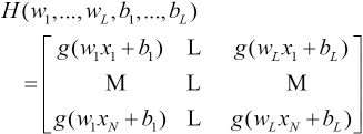
H is the hidden layer output matrix and β is the output weight matrix. The above minimization problem is actually a least squares problem, and Eq. 5, after introducing regularization, becomes as shown in Eq. 8.¹⁷

\min_{β} ∥ H β - T ∥_{F} + \frac{1}{λ} ∥ β ∥_{F}

(Eq. 8)

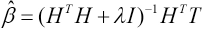
The value of β is given by Eq. 9.

β = H^{†} Y, Y = {[y_{1}, \dots y_{N}]}^{T}

(Eq. 9)

H^† is the generalized inverse matrix of H. Y is the output matrix and actually is equal to T, so the value of β is given by Eq. 10.

\hat{β} = {(H^{T} H + λ I)}^{- 1} H^{T} T

(Eq. 10)

For the new sample x _new , bringing it into the original expression, you can get o_m, where m is the number of categories. The final predicted output value is expressed by Eq. 11.

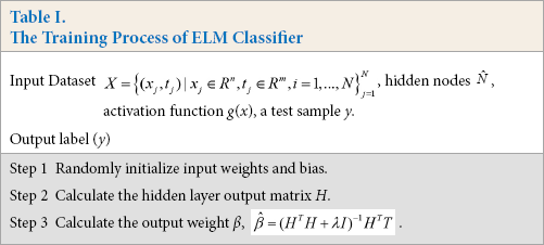
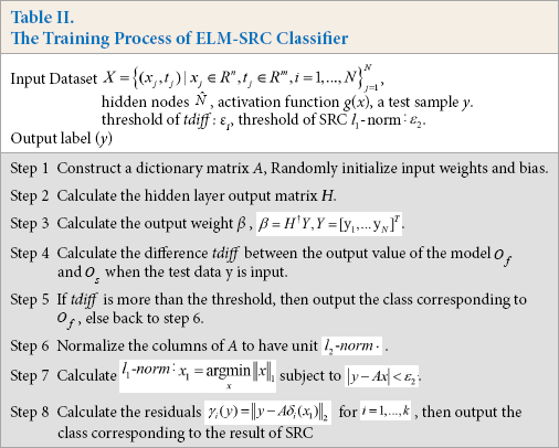
L a b e l (y) = \underset{j \in {1, 2, \dots, m}}{a r g m a x} (o_{j})

(Eq. 11)

We can use Table I to summarize the workflow of the ELM classifier.

Table I

The Training Process of ELM Classifier

Input Dataset $X = {(x_{j}, t_{j}) ∣ x_{j} \in R^{n}, t_{j} \in R^{m}, i = 1, \dots, N}_{j = 1}^{N}$ , hidden nodes $\hat{N}$ , activation function g(x), a test sample y.

Output label (y)

Step 1 Randomly initialize input weights and bias.

Step 2 Calculate the hidden layer output matrix η.

Step 3 Calculate the output weight β, $\hat{β} = {(H^{T} H + λ I)}^{- 1} H^{T} T$

Compared to other classifiers, the biggest advantage of ELM is that the traditional neural network, especially SLFNs, is faster than traditional learning algorithms as well as guaranteeing learning accuracy. However, in practical applications, the ELM model is not robust enough for interference, such as high noise. ELM is a single hidden layer network and once the parameters of the input and hidden layers are set, they will not be changed. If the inputs have noise or disturbance, ELM may make wrong judgments, so its robustness is not very good.

SRC Classifier

The sparse representation model constructs an overcomplete dictionary firstly based on all button training samples, then it uses the sparse linear combination of the dictionary to represent the test samples, and finally the model recognizes and classifies through the reconstruction error. Therefore, the button defect detection problem based on the sparse representation can be regarded as a linear regression problem.

In button defect detection, if the size of a button image is w × h, a two-dimensional matrix, can be converted into a column vector v of dimension m = w × h. Given a training set Z consisting of k categories of samples, where v_i,j ∊ R^m represents the j-th sample of the i-th button, m is the eigenvector dimension of the sample. In the i-th button image, all the column vectors of n_i samples are merged.

According to the linear subspace principle,¹⁸ the test sample y belonging to the i-th class can be approximated as being in the linear space composed of the i-th training samples (Eq. 12).

y = α_{i, 1} v_{i, 1} + α_{i, 2} v_{i, 2} + \dots + a_{i, n_{i}} v_{i, n_{i}}

(Eq. 12)

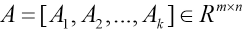
Where $x_{i} = [α_{i, 1}, α_{i}, \dots, a_{i n}] \in R^{m}$ is the sparse coefficient and reconstruction coefficient of the test sample y, corresponding to the i-th training sample.

Because the class of the test sample y is unknown at first, it is necessary to combine the sample set A_i of k classes to obtain a dictionary matrix A (Eq. 13).

A = [A_{1}, A_{2}, \dots, A_{k}] \in R^{m \times n}

(Eq. 13)

$n = \sum_{i = 1}^{k} n_{i}$ represents the total number of samples. At this point, the test sample can be linearly represented by the dictionary matrix A as in Eq. 14.

y = A x

(Eq. 14)

$x = [0, \dots 0, a_{i, 1}, a_{i, 2}, \dots, a_{i, n_{i}}, 0, \dots, 0]$ is the coefficient vector. To achieve the ideal effect of the coefficient representation, all coefficients are 0, except those which correspond to the i-th training sample in the coefficient vector. It can be seen that the coefficient vector itself carries category information of the test samples. Therefore, the class of test sample can be obtained by solving the sparse coefficient of Eq. 14.

It can be seen from Eq. 14 that when the dimension of the dictionary matrix A is m > n, the equation has a unique solution x. This is why all the original data have to be dimensionally reduced in the process of image classification. Therefore, the sparse representation problem can be transformed into an optimization problem, usually solved by minimizing l ₀ - norm, and the optimization model is shown in Eq. 15.

\min_{x} ∥ x ∥_{0} s . t y = A x

(Eq. 15)

$∥ \cdot ∥_{0}$ represents the number of non-zero elements in the sparse coefficient x, but research demonstrates that the solution of the l₀ - norm is an NP-HARD problem. According to the theory of compressed sensing, l₁ - norm minimization can be used to replace the above optimization method.¹⁹ The premise is to satisfy that the coefficient x is sparse enough. So the formula can be converted to Eq. 16.

\min_{x} ∥ x ∥_{1} s . t y = A x

(Eq. 16)

Because Eq. 16 is a standard convex optimization model, in practice, it can be transformed into Eq. 17, where ε is the error allowed.

\min_{x} ∥ x ∥_{1} s . t ∥ y - A x ∥_{2} \leq ε

(Eq. 17)

Compared with other classifiers, SRC is not sensitive to data defects, and the selection of feature space becomes less important. Therefore, SRC has excellent robustness, generalization ability, and anti-interference ability without training.

However, it suffers from complicated calculation and is time consuming due to minimizing the l ₁ norm based on large dictionary matrix A.

ELM-SRC Classifier

In this method, the training process of the ELM is first introduced based on the preprocessed dataset. Then, the ELM model is trained as a classifier for noisy button images by cooperating with the SRC complete dictionary.

On the basis of the ELM classification, for each class, the sample can get the output called o_i. The ELM algorithm considers that the larger the o value, the greater probability that the sample belongs to the class, but the fact is that ELM is difficult to accurately classify images with high noise, so we can define the error classification tdiff in Eq. 18.

t d i f f = o_{f} - o_{s}

(Eq. 18)

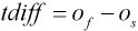
o_f is the maximum value of the output, and o_s is the second largest value of the output. For the two-category problem of this study, there are only two output values, and the larger the value of tdiff, the clearer the boundary of the classification, and the smaller the probability of misclassification. When tdiff is less than a certain threshold, it is considered that the sample is misclassified to a large probability and needs to be sent to SRC for reclassification. This threshold is selected by multiple experiments under the regularization λ = 0.6.

We can use Table II to summarize the workflow of the ELM-SRC classifier. The regularization parameters of ELM are obtained by the five-fold cross-validation method. The specific implementation steps are as follows.

Table II

The Training Process of ELM-SRC Classifier

Input Dataset $X = {(x_{j}, t_{j}) ∣ x_{j} \in R^{n}, t_{j} \in R^{m}, i = 1, \dots, N}_{j = 1}^{N}$ , hidden nodes $\hat{N}$ , activation function g(x), a test sample y. threshold of tdiff: ε₁, threshold of SRC l₁ -norm^: ε₂.

Output label (y)

Step 1 Construct a dictionary matrix A, Randomly initialize input weights and bias.

Step 2 Calculate the hidden layer output matrix η.

Step 3 Calculate the output weight β, $β = H^{†} Y, Y = {[y_{1}, \dots y_{N}]}^{T}$ .

Step 4 Calculate the difference tdiff between the output value of the model

o_f and o_s when the test data y is input.

Step 5 If tdiff is more than the threshold, then output the class corresponding to o _f, else back to step 6.

Step 6 Normalize the columns of A to have unit l₂ -norm.

Step 7 Calculate $l_{1} - n o r m : x_{1} = \underset{x}{a r g m i n} ∥ x ∥_{1}$ subject to $| y - A x | < ε_{2}$ .

Step 8 Calculate the residuals $γ_{i} (y) = ∥ y - A δ_{i} (x_{1}) ∥_{2}$ for i = l,..., k, then output the class corresponding to the result of SRC

First, giving the regular item candidate set λ ∊ {λ_min, λ_max}, the dataset is divided into five parts, four of which are used for model training, and the other one is used for validation. Each validation set can obtain predicted values and calculate their f1-score, then the selected λ is given by Eq. 19.

λ_{s e l e c t} = \underset{λ \in {λ_{\min}, λ_{\max}}}{\arg \min} \frac{\sum_{i = 1}^{5} {(f 1 - s c o r e)}_{i}}{5}

(Eq. 19)

The evaluation criterion f1-score defines the prediction accuracy of the ELM algorithm. F1-score is the harmonic average of the precision and recall rate. We use the f1-score as the evaluation criterion of button defect detection. The larger the f1-score value, the higher the accuracy of the model.

Experiment

Experimental Procedure

The experimental environment was configured as Matlab 2013 and Intel i5 CPU. We designed two methods, ELM and ELM-SRC. First, 1000 test images and 3200 training images, including 2000 positive and 1200 negative samples, were collected by industrial cameras. Ten, the images were prepro-cessed in batches, including eliminating reflection, grayscale, dimensionality reduction, normalization, and so forth.

For the ELM-SRC algorithm, the preprocessed training data constructed a sparse dictionary, and also used the five-fold cross-validation to train the ELM model. The flow chart of ELM-SRC experiment is shown in Fig. 7.

Fig. 7

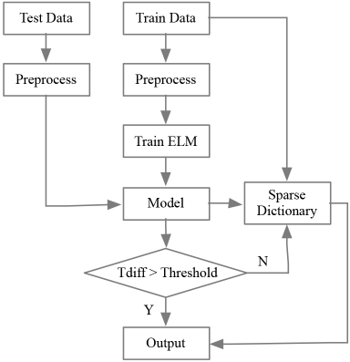
The flow chart of ELM-SRC.

Experimental Results and Analysis

In the first stage, we randomly divided the training set into five parts after preprocessing, four of which were used for training, and the other one was for validation. We selected the regularization parameter of ELM: λ_min = 0.1, λ_max = 1, step = 0.05, then conducted five cross-over experiments, and averaged the parameter values obtained from five experiments. We obtained the averaged f1-score of the validation set under different parameters. The results are shown in Fig. 8.

Fig. 8

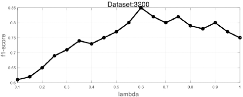
ELM regularization parameters f1-score curve.

From Fig. 8, the best regularization parameter obtained by the experiment was 0.6.

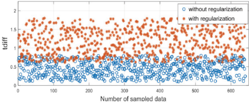
Next, we conducted a five-fold cross-validation experiment on ELM without regularization and with regularization (λ = 0.6). This was done to get its predicted output value o _f and o_s, where o _f is the probability of the positive sample, and o_s is the probability of the negative sample. We obtained tdiff = $t d i f f = | o_{f} - o_{s} |$ of different samples, as shown in Fig. 9.

Fig. 9

ELM and tdiff graph (without regularization and with regularization).

The experimental results show that the larger the tdiff value, the higher the accuracy of the classification. Finally, we gave the predicted results of the ELM and ELM-SRC algorithm on the validation set, as shown in Fig. 10.

Fig. 10

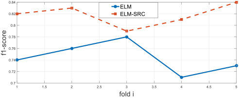
Difference of f1-score between ELM and ELM-SRC.

The f1-score values of ELM-SRC were larger than ELM's. Similarly, on 1000 test samples, we obtained the classification results of ELM and ELM-SRC, while the f1-score of the ELM algorithm was 0.79 and the f1-score of the ELM-SRC algorithm was 0.86.

We compared our method with other methods in terms of running time and detection accuracy. The result is shown in Table III.

Table III

Comparison between Our Method and Others

Method	Precision	Recall	f1-Score	Training Time	Testing Time
ELM	0.714	0.654	0.683	109.7 s	0.28 s
SRC	0.821	0.806	0.813	-	1.58 s
SiameseNet²⁰	0.751	0.728	0.739	15.32 h	0.35 s
Li⁶	0.803	0.794	0.798	-	0.26 s
Our Method	0.857	0.827	0.842	109.7 s	0.76 s

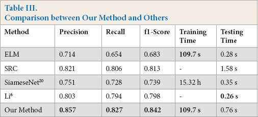
From Table III, although the ELM model took less time to test, the detection accuracy was lower. The SRC model was comparable to our method, but the SRC model took more time than ours when testing. In addition, the SiameseNet²⁰ was time-consuming to train and the detection accuracy was lower. Li⁶ took the least time to test, but the accuracy was lower than ours. Consequently, our method not only achieved the rapidity of button defect detection, but also improved the accuracy.

Conclusions

In this work, we proposed a novel cascaded classifier network with regularized ELM and SRC. First, we adopted an exemplar-based algorithm, Laplace transform algorithm, and PCA to preprocess the metal button images. The five-fold cross-validation method to optimize the regularization parameters of the ELM was then applied. In addition, using the positive and negative samples of the training data and the corresponding labels, we constructed an SRC network with a complete dictionary. The network performed a secondary classification when the ELM output was a high-noise result. This model improved the generalization performance while ensuring the accuracy. Future work will apply the network to the defect detection of shell buttons and plastic buttons, then retrain and fine-tune the network model to achieve better detection performance.

References

Yang

Ph.D. Degree, Fujian Normal University, Fujian, China, 2017.

Chen

; Yap

K.H.

IEEE Transactions on Cybernetics 2014, 44, 695–706.

Chen

M.S. Degree, Huazhong University of Science & Technology, Wuhan, China, 2015.

Zhou

Ph.D. Degree, Huazhong University of Science & Technology, Wuhan, China, 2016.

Burges

A. C. J. C.

Data Min. Knowl. Discov. 1998, 2, 121–167.

Technology Innovation and Application 2018, 8, 2–4.

Zheng

; Kong

L.X.

; Nahavandi

Journal of Materials Processing Technology 2002, 125, 427–433.

Huang

G.B.

; Zhu

Q.Y.

; Siew

C.K.

Neurocomputing 2006, 70, 489–501.

Huang

; Zhu

; Siew

C.-K.

Neural Networks 2004, 2, 985–990.

10.

Wright

; Yang

; Ganesh

; Sastry

S.S.

; Ma

IEEE Trans. Pattern Anal. Mach. Intell. 2009, 31 (2), 210–227.

11.

Cao

; Zhang

; Luo

; Yin

; Lai

Neural Networks 2016, 81, 91–102.

12.

Wang

Ph.D. Degree, Beihang University, Beijing, China, 2013.

13.

Xiao

; Zhou

IEEE Transactions on Neural Networks and Learning Systems 2018, 30 (7), 1–15.

14.

Huang

G.B.

; Ding

; Zhou

Neurocomputing 2010, 74, 155–163.

15.

Huang

G.-B.

; Siew

C.-K.

Proc. 8th Int. Conf. Control, Autom. Robot. 2004, 2, 1029–1036.

16.

Heeswijk

; Miche

Neurocomputing 2015, 149, 187–197.

17.

Zheng

; Shu

Signal Processing 2013, 29 (7), 888–895.

18.

Candes

E.J.

; Romberg

; Tao

IEEE Trans. Inform. Theory 2006, 52 (2): 489–509.

19.

Dai

Q.H.

; Fu

C.J.

; Ji

X.Y.

Chinese Journal of Computers 2011, 34 (3), 425–434.

20.

Zagoruyko

; Komodakis

Computer Vision and Pattern Recognition 2015, 4353–4361.

Method of Metal Button Defect Detection Based on Extreme Learning Machine and Sparse Representation

Abstract

Keywords

Introduction

Image Preprocessing

Collecting Images

Eliminating Reflection

Edges Extraction and Dimensionality Reduction

ELM-SRC Network Model

ELM Classifier

SRC Classifier

ELM-SRC Classifier

Experiment

Experimental Procedure

Experimental Results and Analysis

Conclusions

References