Sage Journals: Discover world-class research

Abstract

The software-defined networking paradigm enables wireless sensor networks as a programmable and reconfigurable network to improve network management and efficiency. However, several challenges arise when implementing the concept of software-defined networking in maritime wireless sensor networks, as the networks operate in harsh ocean environments, and the dominant underwater acoustic systems are with limited bandwidth and high latency, which render the implementation of software-defined networking central-control difficult. To cope with the problems and meet demand for high-speed data transmission, we propose a radio frequency–acoustic software-defined networking-based multi-modal wireless sensor network which leverages benefits of both radio frequency and acoustic communication systems for ocean monitoring. We first present the software-defined networking-based multi-modal network architecture, and then explore two examples of applications with this architecture: network deployment and coverage for intrusion detection with both grid-based and random deployment scenarios, and a novel underwater testbed design by incorporating radio frequency–acoustic multi-modal techniques to facilitate marine sensor network experiments. Finally, we evaluate the performance of deployment and coverage of software-defined networking-based multi-modal wireless sensor network through simulations with several scenarios to verify the effectiveness of the network.

Keywords

Software-defined networks wireless sensor networks ocean monitoring underwater sensor networks multi-modal networks

Introduction

As the ocean has made a significant contribution to the world economy, there has been a great surge of interest in ocean exploration.^1,2 To facilitate the in situ ocean observation, wireless sensor networks (WSNs) are deployed in the ocean in the form of ocean sensor networks (OSNs), which have a wide range of applications, such as ocean environmental monitoring, assisted navigation, scientific research, disaster prevention, and maritime military operations.³ Generally, except being deployed on the ocean surface, OSNs are also being deployed in the water, which is termed as underwater wireless sensor networks (UWSNs).¹ However, to facilitate the ocean exploration further with these networks, we may consider a paradigm shift by applying novel emerging techniques, because currently, most of the OSNs are with rigid, closed, and inflexible architectures, which are hard to reprogram, reconfigure, and update once deployed in the ocean.

Software-defined networking (SDN) is considered as one of such emerging architectures with promising advantages compared to traditional networks, which offers a new networking paradigm by separating the control plane from the data plane.⁴ Leveraging a global view of the whole network, researchers may harvest potential benefits, such as improving energy efficiency, simplifying network management, as well as enhancing assets interoperability and network evolution.⁵ Coupled with other software-defined technologies, for example, network function virtualization (NFV) and software-defined modem (SDM), SDN-based OSNs are also able to support multi-application networks. In such way, the conventional networks are transformed toward user-customizable, programmable, and service-oriented next-generation ocean monitoring networks.⁵

Although SDN has recently attracted much attention from the research community, new challenges arise when the original SDN concept is applied to ocean monitoring systems. The original SDN is ensured by reliable centralized control, but as the primary communication technology used in OSNs is acoustic currently, the implementation of centralized control faces several challenges. First, the unreliable underwater acoustic communication links incur uncertainty to the process of both network information collection and control message dissemination. Second, the underwater acoustic signal suffers severe propagation delay due to its slow transmission speed that is approximately 1500 m/s. Such a lengthy delay may render central control useless especially in response to emergency events in real-time when sensor nodes need to take actions immediately. Third, the separated control plane leads to extra control communication overhead as OSNs are mostly deployed in a highly dynamic underwater environments (e.g. spatio-temporal varying communication channels and frequent node mobility). This not only introduces considerable control overhead, but also results in serious performance degradation under limited underwater acoustic bandwidth.

Since underwater acoustic communication has inherent constraints, such as significant delay, high energy consumption, and low data rate, it cannot meet the huge demand for high-speed data transmission of emerging applications (e.g. real-time video, high definition (HD) images, and real-time control and synchronization). To overcome the drawbacks of acoustic technology, researchers are prompted to develop other non-acoustic alternative communication technologies, such as optical, radio frequency (RF), and electromagnetic (EM).⁶ However, these newly developed technologies also have their shortcomings. For example, compared to acoustic communication, the optical system enables high data rate, ultra-low delay and energy efficiency, and it also suffers from short-range wireless communications (e.g. less than 200 m in the deep ocean). Nevertheless, the paradigm of SDN supports multi-modal wireless technologies,^7–9 and as multi-modal design seeks to find solutions of combining different technologies to compensate for drawbacks of a given communication system, it is possible to meet the growing demand of diverse application requirements.

To overcome the above-mentioned problems of ocean monitoring, especially the monitoring of both ocean surface and beneath the ocean, we incorporate the RF and acoustic multi-modal communication systems into the SDN paradigm, and propose an SDN-based multi-modal wireless sensor network (SM-WSN) architecture for ocean monitoring. The initial work was in the study of Luo et al.,^2,10 and we extend it further in this article. Based on the proposed network architecture, to deal with the challenges of implementing central control of SDN in harsh ocean environments, we propose a semi-centralized control mechanism to improve control flexibility and reliability. Then, we explore two examples of SM-WSN: the deployment and coverage issues in intrusion detection, and a novel RF and acoustic testbed solution. We first discuss the deployment issue of SM-WSN, and present a coverage analysis under surveillance scenario of intrusion detection with both grid-based and random deployment, in which we leverage the floating radius to enlarge detection area and reduce deployed nodes. After that, we present a novel SDN-based multi-modal testbed design, in which we incorporate RF–acoustic multi-modal technologies to facilitate marine sensor network experiments.

The main contributions of this article are summarized as follows:

We present an SM-WSN architecture that leverages the ocean surface RF channel and underwater acoustic channels to satisfy diverse application demands.

We provide a mathematical analysis of deployment and coverage issues for marine intrusion detection with grid and random deployed SM-WSN.

We propose an SDN-based marine testbed for real ocean scenarios by implementing multiple RF and acoustic communication techniques to improve the flexibility and adaptability of the ocean monitoring testbed.

The rest of the article is organized as follows. In “The basic architecture design” section, we present the basic architecture of SM-WSN. In “The deployment of SM-WSN for intrusion detection” section, we describe the deployment issues of SM-WSN with intrusion detection scenarios. The testbed design is presented in the “Testbed design of SM-WSN” section. We provide evaluations and experiments in the “Deployment and coverage performance evaluation” section. The related state-of-the-art research is reviewed in the “Related work” section. Finally, in the “Conclusion” section, we give the conclusions.

The basic architecture design

In this section, the basic architecture of SM-WSN is described first, and then we present the details of both semi-centralized control and network node design. The list of acronyms and symbols are presented in Tables 2 and 3 in Appendix 1, respectively.

The basic architecture of SM-WSN

As depicted in Figure 1, the integrated architecture primarily includes: data plane, control plane, and application plane.^7,11 To facilitate decision-making and improve the flexibility of the architecture, cross-layer information sharing is also implemented among all the functional modules and planes. This architecture separates the different functions of the network, and at the same time, it also shares the information among different layers, especially from the physical systems and the communication environments to increase network adaptivity.

Figure 1.

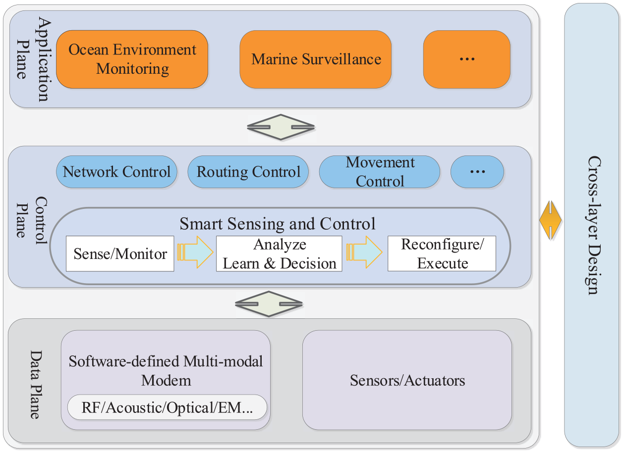
An architecture of integrated SDN and multi-modal network.

In the data plane, the multi-modal communication systems (e.g. RF, optical, and acoustic communication) are designed using SDM techniques. As shown in Table 1, different wireless communication technologies have their pros and cons, but these systems are also complementary to each other, so that, we are able to exploit their complementary characteristics with SDN architecture. Besides, the network sensors sense the environment, while actuators execute optimized decisions which come from the decision-making components.

Table 1.

Characteristics of multiple communication technologies.

Technologies	Range	Data rate	Latency	Energy	Weakness	Advantages
RF	~100 m	~Kbps	0.003 ms/km	50,000 bits/Joule	Affected by waves, severe weather, for example, storm	High data rate, low latency, low energy consumption
Acoustic	~km	~Kbps	667 ms/km⁸	100 bits/Joules¹²	High delay, low bandwidth	Long communication range
Optical	~100 m	~Mbps	0.03 ms/km⁸	30,000 bits/Joules¹²	Line-of-sight, tight alignment	High data rate, low latency, low energy consumption
EM	~10 m	~Mbps	0.03 ms/km⁸	–	Large antenna, very short communication range	Non-line-of-sight, cross boundary communications

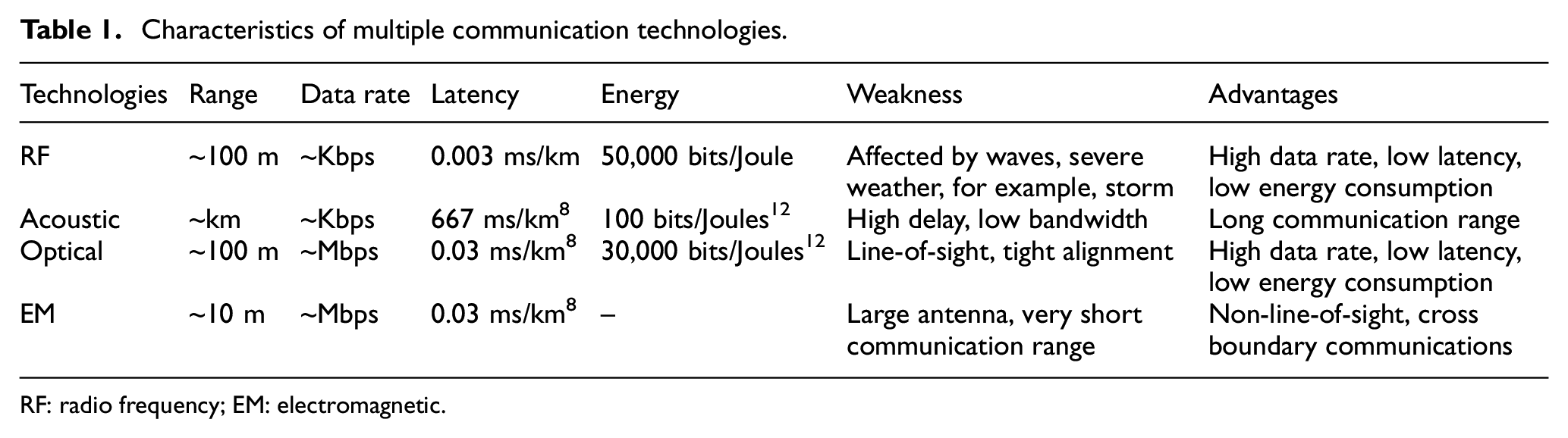
RF: radio frequency; EM: electromagnetic.

In the control plane, the smart sensing and control component serves as the local brain of the network. It consists of several parts, such as sensing and monitoring, analyzing and decision-making, reconfiguration, and executing. To perform sensing and monitoring, the timely raw data are provided by the sensors, which come either from the environment or from the feedback of the control operations of the network. To enable the decision core to perform intelligently, several artificial intelligence (AI) and data-driven tools, such as machine learning, reinforcement learning, could be incorporated into the decision-making component.

In the application layer, diverse applications are able to be performed, such as ocean environment monitoring, maritime surveillance, and so on. To meet the diverse demands of the application layer, and improve the network efficiency, multiple applications may be deployed in the same network leveraging NFV techniques.⁵

The semi-centralized control

There are several control techniques in SM-WSN, such as centralized, distributed, and semi-centralized control.¹³ Generally, semi-centralized control combines the advantages of both centralized and distributed control, so as to provide network control flexibility.

Although centralized control may perform well with limited nodes and a small network,¹⁴ its performance may be compromised especially with frequent topology changes of OSNs.^15,16 The drawback of the fully centralized control is also verified in terrestrial WSNs in the work of Buratti et al.,¹⁷ in which experimental tests are conducted to compare SDN-based WSN with two typical solutions: Zigbee and 6LoWPAN. The results show that SDN-based WSNs lead to performance degradation under highly dynamic conditions due to the increment of the control overhead. The authors in Guo et al.¹⁸ also pointed out that strict separating data plane from control plane may not be well-suited to WSNs considering its inherent characteristics, such as unreliable communication channel and dynamic nature of mobile networks.

To solve the above-mentioned problem, one feasible solution is to divide the control management among sensor nodes and the controllers, which is termed as semi-centralized control.⁵ By combining the centralized control and the distributed control, the essence of the semi-centralized control is to keep a certain level of self-control capability of sensor nodes while benefiting from the advantages of centralized control.¹⁹ Hence, it not only exploits the ad hoc nature of sensor networks to reduce the control message overhead, but also improves the network robustness and control efficiency.^18,20

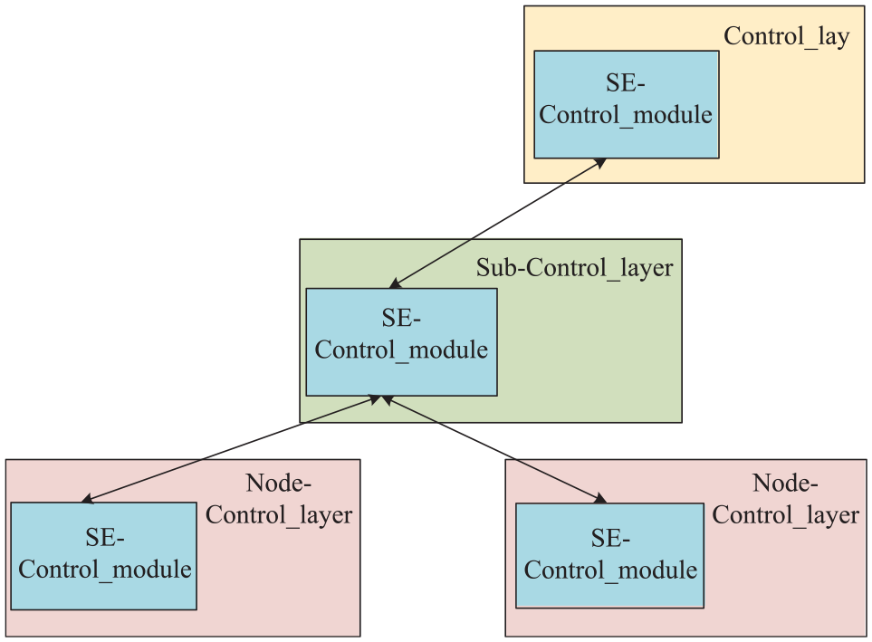
The implementation of the semi-centralized control primarily includes three components: the semi-centralized control module, the smart sensing and control module, and the multi-modal communication module. The semi-centralized control is deployed in three levels, as shown in Figure 2. The first-level control resides in the central control center, such as underwater or floating sinks, unmanned surface vehicles (USVs), and so on. The second-level control is deployed in the cluster-header node and the third-level control is implemented in the cluster member nodes. Among the three levels of control, the first-level control takes charge of the overall optimized control of the network. The second-level control primarily implements the centralized controls from the central controller, and at the same time, it is also capable of making decisions based on its in situ environment. Similarly, the third-level control also has the local flexibility of self-distributed control as well as the central control. Overall, the three-level control architecture requires coordinated control among these three levels. By leveraging the control channel and the control module, the strategy of semi-centralized control is implemented in a hybrid of centralized and ad hoc fashion.

Figure 2.

The semi-centralized control.

The semi-centralized control requires smart nodes to perform intelligent sensing, networking, data processing and control. Therefore, these smart nodes not only execute instructions from the control center, but also have self-adaptive capabilities to cope successfully with extreme environments and carry out specific tasks efficiently and effectively. Empowered by the local brain, the network node coordinates smart sensing, data analyzing, decision-making, resource reconfiguration, smart control, and executing intelligently, which will reduce the costly communication overhead in favor of complex computing.

The network node design

Based on the basic architecture of SM-WSN, we develop an RF–acoustic multi-modal node that combines both RF and acoustic communication systems. To note that, our design considers the characteristics of ocean monitoring in which we aim at both ocean surface monitoring and underwater monitoring, especially for two examples of SM-WSN in the following sections, such as the intrusion detection and SDN-based ocean monitoring testbed. Nevertheless, based on the architecture of SM-WSN, other multi-modal network nodes can be designed according to different application scenarios and requirements. For example, mobile multi-modal nodes, such as autonomous underwater vehicles (AUVs) can leverage both acoustic and optical communication technologies.

As exhibited in Figure 3, the multi-modal node includes a floating buoy, a mooring line, an underwater anchor, and a number of underwater acoustic sensors which are attached to the mooring line and form a group node. Although the sensors along the mooring line could be wired to expensive special mooring cables, it has shortcomings, such as cable breakage. It is a robust and cost-effective alternative to utilize the wireless acoustic technique in the network. Actually, it is also a linear acoustic sensor network formed by the attached sensors along the mooring line. Meanwhile, the acoustic node communicates directly with its adjacent sensors which are in its communicating range. To note that, the surface nodes are equipped with multi-modal communication systems, that is, RF system²¹ and underwater acoustic system.⁶ Therefore, the network is a two-tier hybrid network. One tier is over the ocean surface via RF communication, and the surface stochastic link modeling is presented in the work of Shahanaghi et al.²² Meanwhile, the other tier is underwater via acoustic technique.

Figure 3.

A schematic RF–acoustic multi-modal node design and deployment.

As the surface sensor node resides in the floating buoy, it is not stationary but moves within a restricted area after deployment. As depicted in Figure 3, the node would move randomly around the underwater anchor center driven by the combined forces, such as the wind, the ocean waves, and the mooring line. Among these forces, the ocean waves are the critical factor affecting the float drifting model. However, precisely acquiring the ocean movement model is difficult, though we have known multiple primary factors which have some effect on the model (e.g. wind, salinity, and temperature). However, Caruso et al.²³ integrated looping and downstream motions into the ocean movement, and obtained a simplified model in accordance with the following equation

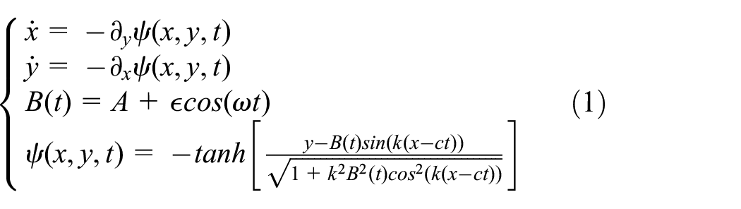
{\begin{matrix} \overset{\cdot}{x} = - \partial_{y} ψ (x, y, t) \\ \overset{\cdot}{y} = - \partial_{x} ψ (x, y, t) \\ B (t) = A + ϵ \cos (ω t) \\ ψ (x, y, t) = - \tanh [\frac{y - B (t) \sin (k (x - ct))}{\sqrt{1 + k^{2} B^{2} (t) co s^{2} (k (x - ct))}}] \end{matrix}

(1)

where k, c, ε, and ω represent meander numbers, phase speed, amplitude, and frequency of modulation, respectively.

The deployment of SM-WSN for intrusion detection

Intrusion detection is one primary part of the security surveillance system with potential applications ranging from border security, commercial facilities protection, harbor protection, and maritime surveillance.^5,24–26 In maritime surveillance, the intrusion detection system should detect invaders on the sea surface, such as boats, ships, as depicted in Figure 4.

Figure 4.

A sample of ship intrusion detection with grid-based deployment.

Furthermore, the system should detect underwater intruders, such as remotely operated vehicles (ROVs), AUVs, and even divers to enhance maritime safety and security. Inspired by the building of terrestrial wireless sensor barriers to deter intruders penetrating into the protected area, we focus on the construction of a marine barrier with SM-WSN to perform three-dimensional intrusion detection functions.

To simplify the deployment, we consider both the grid-based and random deployment, as shown in Figure 5. It is clear that in grid-based deployment, the network is efficient and simple for maritime surveillance. However, random deployment may be the feasible solution under certain scenarios. We first present the free-drifting radius and the sensing model, and then describe the deployment and coverage problems on two scenarios: grid- and random-based deployment.

Figure 5.

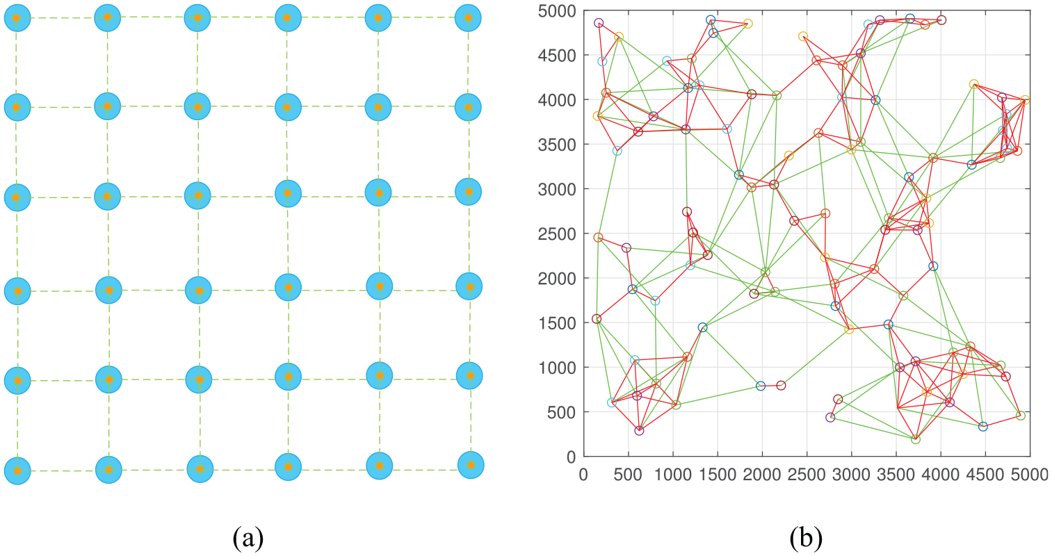
Samples of grid and random deployment. (a) Grid-based deployment and (b) random deployment.

The free-drifting radius and sensing model

After the surface node is deployed, since it is with the floating buoy, the node is not stationary but drifts freely within a restricted area on the sea surface. We calculate the free-drifting radius of the sensor node. Let h represent the depth of the sea, l is the mooring line length, and r presents the floating radius of the drifting circle. Using the right-angled triangle theorem, r is calculated as $r = \sqrt{l^{2} - h^{2}}$ .

In practical deployment, to prevent the rope line from breaking, the rope usually has a residual length which is longer than the maximum depth of the ocean, denoted as l_m. Since the tide incurs the rise and the fall of the ocean surface level, the sea depth is not constant, but has the highest and the lowest ocean level. Accordingly, let h_max and h_min represent the highest and the lowest sea depth, respectively. Thus, the sea depth satisfies h∈ {h_min, h_max}. Accordingly, the rope length should be l = h + l_m. Consequently, the varying sea depth incurs varying floating radius r. Let r_min and r_max represent the minimum and maximum floating radius, respectively. The radius r∈ {r_min, r_max}. And r_min and r_max are obtained by the following equations

{\begin{matrix} r_{\max} = \sqrt{l^{2} - h_{\min}^{2}} \\ r_{\min} = \sqrt{l^{2} - h_{\max}^{2}} \end{matrix}

(2)

Different types of sensing models appeared in the literature, as shown in Figure 6, such as binary sensing model and probabilistic sensing model.^27,28 However, the binary sensing model is also a special case of the probabilistic model. Typically, in terms of a probabilistic model, the probability of the target t detected by a sensor i satisfies the following equation

p_{i} = {\begin{matrix} 1, d_{i} \leq μ_{1} \\ e^{- α (d_{i} - μ_{1})}, μ_{1} < d_{i} \leq μ_{2} \\ 0, d_{i} > μ_{2} \end{matrix}

(3)

where d_i is the distance between the target t and sensor i, and µ₁ is the starting uncertainty sensing point, and µ₂ represents the maximal sensing range. The parameter α is associated with the physical properties of the detecting sensor as well as its deployment environment which can be obtained via experiments.^28–30 In equation (3), if µ₁ = µ₂, the probabilistic sensing model turns into the binary sensing model, as shown in Figure 6. Generally, the binary sensing model is simple and its deterministic sensing range is shorter than the probabilistic model as it excludes the uncertain sensing range. So, with the binary sensing model, there is always needs to deploy more detection sensors to achieve full coverage.

Figure 6.

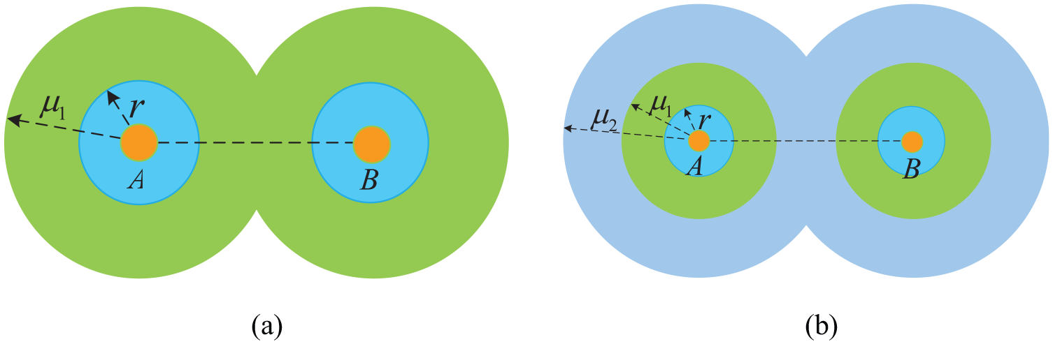
Two types of sensing models: (a) the binary sensing model and (b) the probabilistic sensing model.

Nevertheless, in many application scenarios, we may leverage the sensing uncertainty via the probabilistic sensing model to reduce deployed sensors upon the network satisfies the minimum detection threshold. For example, if the number of sensors that have detected the target is N, N∈ {1,2,…, n}, the probability of detection of the target is

p = 1 - Π_{i = 1}^{n} (1 - p_{i})

(4)

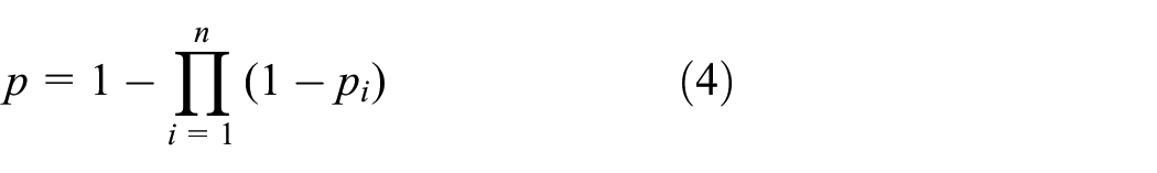
If we assume that the target detection probability is no less than p_min, then we have p ≥ p_min.

The grid-based deployment scenario

We describe the grid-based deployment scenario, and first analyze the floating barrier coverage issue theoretically. Then, we obtain the minimal nodes covering the targeted detection area fully. After that, we present a brief case study of surface intrusion detection and explore underwater coverage of the floating barrier.

Surface coverage of the floating network

As depicted in Figure 4, we consider a grid-deployed barrier belt with surface nodes, and the nodes communicate with each other using RF channels. To provide some insights on how to cover the targeted areas, we simplify the coverage analysis model of the network, and the nodes have the same deployment characteristics. The length of the mooring rope is l, and the sea depth is denoted as h, thus, the maximum floating radius r is similar. We also assume that the sensing and communicating ranges are identical. Although, both the sensing range and communication range are not a perfect circle in reality, the circle model could be used to approximate the reality, so as to obtain coverage bounds for real deployment. The sensing range and the communication range are denoted as R_sen and R_com, respectively. To note that, under the probabilistic model with equation (3), if µ₁ = µ₂ = R_sen, the sensing model turns into a binary model, and if R_sen is the maximum sensing range, it is still a probabilistic model.

To detect intruders on the ocean surface, for example, boats, ships, swimmers, USVs, k-barrier coverage could be used as a quality metric for the surface belt barrier intrusion detection.³¹ When an intruder attempts to cross the belt barrier in any direction, as shown in Figure 4, if the intrusion event is sensed by at least k (k ≥ 1) sensors, the belt barrier achieves k-barrier coverage. As the floating barrier is deployed in the ocean, and the surface nodes are in grid-based deployment which is formed by a number of parallel lines, when the intruder traverses across one barrier line, if the intruder is detected by at least one sensor, we say that the sensor barrier achieves one-barrier coverage. Since we deploy a number of parallel barrier lines around the target area, two parallel lines around the target area form fully one-barrier coverage. Therefore, to achieve k-barrier coverage, we have to deploy k + 1 parallel lines of sensors.

To achieve full coverage, as depicted in Figure 4, the surveillance area is divided into many square lattices. We consider the lattices formed by two adjacent parallel lines, as shown in Figure 7, and a square lattice is formed by four adjacent deployment nodes. In the figure, four points A, B, C, and D represent both four group nodes and their deployment positions of the anchors. Because the floating sensor node will drift freely within a restricted area after the initial deployment, two adjacent sensor nodes should have enough deployment distance to keep them from tangling with each other as they are attached to mooring lines. As an example, we denote the distance between nodes A and B as L_AB, and it satisfies the equation below

\begin{matrix} L_{AB} > 2 r \\ = 2 \sqrt{l^{2} - h^{2}} \end{matrix}

(5)

Figure 7.

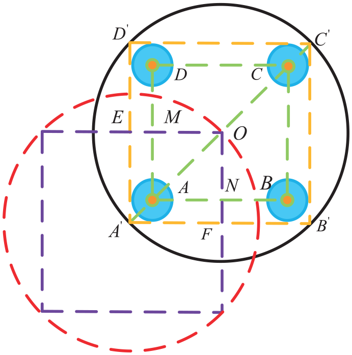
Surface coverage with grid-based deployment.

To achieve full one coverage, each point in the square ABCD should be covered by at least one node that is deployed at the four vertices of the square. Next, we obtain sufficient conditions of the full coverage. In the following theorem, it is mathematically proved that, when $R_{sen} \geq \sqrt{2} \sqrt{l^{2} - h^{2}} + \frac{\sqrt{2}}{2} L_{AB}$ , the square is fully covered by four nodes at the square’s four vertices. We present the theorem and the proof as follows.

Theorem

In a square grid, to achieve full coverage of the square area formed by four nodes at the square vertices, the sensing range R_sen of the four nodes should satisfy the condition below

R_{sen} \geq \sqrt{2} \sqrt{l^{2} - h^{2}} + \frac{\sqrt{2}}{2} L_{AB}

(6)

Proof

As shown in Figure 7, □ABCD is formed by point A, B, C, D, and its side length is L_AB. We stretch four points outward horizontally and vertically as r, respectively, and enlarge the square to a new □A′B′C′D′ as shown in Figure 7. The square circumscribed the four small circles whose radius equals to r.

According to geometry theorems about regular polygons and circles, a square has a unique circumcircle. The radius of the circle equals to the length of the diagonal, and we denote it as R. Meanwhile the circle is centered at point O, which is the intersection point of two diagonals of the square.

We move □A′B′C′D′ and its circumscribed circle ⊙O along diagonal line C′A′ toward point A′ until the center of the circle reaches the vertex point A′ of □A′B′C′D′. Two circles and two squares intersect with each other, as shown in Figure 7, and generate two new small squares □A′FOE and □ANOM. Their area is one quarter of □A′B′C′D′ and □ABCD, respectively. From the figure, the circle centered at A′ with radius R covers the small square □A′FOE and □ANOM fully. We then move the circle ⊙A′ toward the small circle ⊙A and make the center A′ within the small circle ⊙A. In the following, we prove that, centered at any point in ⊙A, the resulting new circle with radius R can still cover the squares □A′FOE and □ANOM.

For ∀P∈□A′FOE, ∀Q∈⊙A, as P∈⊙A′, we have PA′ < R. Connecting points P and Q, and points P and A′, respectively, and hence PQ < R. Thus, the circle centered at Q with radius R covers point P. Therefore, we have proved that if we construct a new circle centered within the circle ⊙A with radius R, the square □A′FOE and □ANOM are fully covered by the new circle. Similarly provable, centered at points B′, C′, D′ with radius R, three circles fully cover the three quarters of the remaining □ABCD. Next, we compute the radius R as the following equation

\begin{matrix} R = \frac{1}{2} L_{A' C'} \\ = \frac{\sqrt{2}}{2} (2 r + L_{AB}) \\ = \sqrt{2} r + \frac{\sqrt{2}}{2} L_{AB} \\ = \sqrt{2} \sqrt{l^{2} - h^{2}} + \frac{\sqrt{2}}{2} L_{AB} \end{matrix}

Therefore, with $R_{sen} \geq R, i . e ., R_{sen} \geq \sqrt{2} \sqrt{l^{2} - h^{2}} + \frac{\sqrt{2}}{2} L_{AB}$ , and the theorem is proved. □

To obtain full coverage of the deployment, we combine equations (5) and (6), and the distance between two adjacent nodes L_AB should satisfy the following condition

2 \sqrt{l^{2} - h^{2}} < L_{AB} \leq \sqrt{2} R_{sen} - 2 \sqrt{l^{2} - h^{2}}

(7)

Next, to cover a given detection target area fully, we deduce the minimum number of nodes. We assume that the target belt is in a grid-based deployment within an L × W surveillance area. Through the surface coverage analysis, the coverage depends both on the distance between two adjacent sensors and on the sensing range R_sen.

When we set R_sen = µ₁ = µ₂, using equation (7), the minimum number of sensors N_min is

N_{\min} = ⌊ \frac{L}{\sqrt{2} R_{sen} - 2 \sqrt{l^{2} - h^{2}}} ⌋ ⌊ \frac{W}{\sqrt{2} R_{sen} - 2 \sqrt{l^{2} - h^{2}}} ⌋

(8)

Case study of surface intrusion detection

In this subsection, we discuss intrusion detection further based on grid deployment and the probabilistic sensing model. As shown in Figure 4, when an intruder (e.g. a ship) moves across the sea surface, multiple nodes would detect the intruder in the grid-deployed network. As mentioned above, leveraging sensing uncertainty via a probabilistic sensing model can reduce the total number of deployment sensors.

We take four sensor nodes in the grid network to illustrate the detection scenario, as shown in Figure 8. In equation (3), d_i denotes the distance between sensor i and target t. And the positions of the target and sensor i are denoted as (x, y) and (x_i, y_i), respectively. If d_i < µ₁, the detection probability is 1. When d_i is between µ₁ and µ₂, the detection probability is less than 1 as sensing uncertainty is involved. As depicted in Figure 8, since the floating sensor has its restricted drifting radius r, the farthest distance between the detecting sensor and the target is denoted as d_max, which satisfies the following equation

d_{\max} = \sqrt{{(x - x_{i})}^{2} + {(y - y_{i})}^{2}} + r

(9)

Figure 8.

Joint detection probability of floating sensors.

We assume that the number of sensors which join to detect the intrusion is N, and P is denoted as the joint detection probability as follows

P = 1 - Π_{i = 1}^{N} (1 - e^{- α (d_{i} - μ_{1})})

(10)

As illustrated in Figure 8, the number N = 4, and the deployment distance L_AB is 200 m, l = 96 m, h = 90 m, and the yellow area represents the area of d_i < µ₁ with detection probability of 1. Although other areas are less than 1, if the joint detection probability P is higher than p_min, the total detection probability still satisfies the requirement of the specific applications.

Three-dimensional underwater coverage

We explore underwater coverage of the floating barrier, and instead of communicating via RF channel in the ocean surface barrier, the networking technique of the underwater barrier is acoustic waves. The goal of the underwater barrier is to detect the intruders while they attempt to break through the underwater barrier. We first present the underwater coverage theoretical analysis for surveillance intrusion detection, and then deduce the full coverage conditions of the underwater barrier.

Instead of covering the whole underwater body, we only need to cover two vertical faces of the cubic body formed by the underwater barrier, which is intersected with the path of the underwater intruders. In other words, if the underwater intruders attempt to cross the three-dimensional underwater barrier, these intruders have to break through one of two sides of the barrier, just like breaking through a wall from either side.

To analyze the coverage properties of the underwater barrier, we project one side of the barrier to a vertical projection plane for the theoretical analysis. Figure 9 shows the part of the barrier projected on the vertical projection plane formed by four adjacent nodes A, B, E, and F. Nodes A and F are within a group node, and are attached to the same mooring line. Whereas, nodes B and E are in another group node, which are attached to the same mooring line. Nodes A and B are deployed on the ocean surface, whereas nodes F and E are deployed underwater. To note that, to perform full three-dimensional coverage, the surface nodes are equipped with multi-modal networking techniques, that is, RF and acoustic.⁶

Figure 9.

The vertical projection of the underwater network.

Next, we calculate the sufficient conditions for full coverage of the vertical plane underwater. Since nodes F and E are the nearest underwater nodes to their separated surface nodes A and B within their group, as shown in Figure 9, they have the maximum free-drifting radius. Thus, the coverage conditions, which are deduced with nodes F and E, are sufficient for other nodes beneath them underwater along the mooring lines. To simplify the analysis, the underwater nodes are assumed in the same group and are attached along the mooring line evenly spaced, thus, the span between nodes F and A denotes as Δh. The number of nodes in each mooring line is denoted as N_l, then we have Δh = l/N_l. The maximum free-drifting radius of nodes A and B is r, and the maximum drifting radius of node E′s and F′s are r_E, r_F, respectively. With geometry theorems, we get

r_{F} = \frac{h - Δ h}{h} r

(11)

Both nodes B and F have restricted free-drifting area and L_B′F′ is denoted as the maximum range between nodes B and F, RU_sen is denoted as the node’s sensing range. To cover the area formed by four vertical nodes, we have

\begin{matrix} R U_{sen} > \frac{1}{2} L_{B' F'} \\ = \frac{1}{2} \sqrt{{(L_{AB} + r_{F} + r)}^{2} + {(Δ h)}^{2}} \\ = \frac{1}{2} \sqrt{{(L_{AB} + \frac{h - Δ h}{h} r + r)}^{2} + {(Δ h)}^{2}} \\ = \frac{1}{2} \sqrt{{(L_{AB} + \frac{2 h - Δ h}{h} \sqrt{l^{2} - h^{2}})}^{2} + {(Δ h)}^{2}} \end{matrix}

(12)

To cover the whole three-dimensional monitoring target area underwater, we combine both the surface and underwater coverage and have the following equation

\begin{matrix} R U_{sen} > \frac{1}{2} \sqrt{{(2 R)}^{2} + {(Δ h)}^{2}} \\ = \frac{1}{2} \sqrt{{(2 \sqrt{2} \sqrt{l^{2} - h^{2}} + \sqrt{2} L_{AB})}^{2} + {(Δ h)}^{2}} \end{matrix}

(13)

The random deployment scenario

We briefly discuss the random deployment scenario. First, we describe the sensing area of a single floating node, and then analyze the surface coverage of the random deployment.

The sensing area of a floating node

The floating area of a sensor node is assumed as a circle area in which the circle center is the anchor deployment position and the radius is r, as shown in Figure 10. We assume that the sensing range is denoted as R_sen, and the distance between the anchor position and the target is D. As shown in Figure 10, when the target is within the area under the condition that D is less than R_sen−r, it will be covered surely.

Figure 10.

The sensing area of a floating node.

Since the surface node appears in its restricted floating area in a uniform distribution for a long-term deployment scenario,³² the rest area will be covered with a probability that is dependent on its instantaneous floating position. We denote the coverage probability as P_a, and when D is between R_sen−r and R_sen + r, its coverage probability is calculated from the following equation according to Heron’s formula³³

f (R_{sen}, r, D) = \frac{ζ - \sqrt{\frac{[{(R_{sen} + r)}^{2} - D^{2}] [D^{2} - {(R_{sen} - r)}^{2}]}{4}}}{π r^{2}}

(14)

where $ζ = \arccos \frac{R_{sen}^{2} + D^{2} + r^{2}}{2 R_{sen} \times D} R_{sen}^{2} + \arccos \frac{r^{2} + D^{2} - R_{sen}^{2}}{2 r \times D} r^{2}$

Figure 11 shows the coverage probability with different D, floating radius and sensing range, and the coverage probability of the sensing area of a floating node can be calculated from the following equation

P_{a} = {\begin{matrix} 1, D < R_{sen} - r \\ f (R_{sen}, r, D), R_{sen} - r \leq D \leq R_{sen} + r \\ 0, D > R_{sen} + r \end{matrix}

(15)

Figure 11.

The coverage probability.

Random deployment analysis

Random deployment may be the only feasible deployment solution under certain scenarios in which it is difficult to deploy monitoring sensors manually. We assume that the network is randomly deployed with a uniform distribution. To get a higher sensing coverage, we should increase the nodes’ density with a fixed sensing distance. However, there is a risk of entanglement when two adjacent nodes are too close. Alternatively, when we leverage the random deployment strategy to build the floating barrier, it is more likely to be a sparse deployment, as shown in Figure 12.

Figure 12.

A sample of sparse deployment.

To construct a floating barrier via these sparsely deployed sensors, it should first form a connected WSN. The good news is that though RF communication range might be shorter, the multi-modal sensors have long-range acoustic communications to connect the sparse network. In addition to the communication connection range, the sensing range obviously influences the effective coverage. As shown in Figure 13, it is observed that with the same random distribution, as the sensing range increases the coverage probability also increases, especially via larger floating drifting radius.

Figure 13.

A sample of a long sensing range.

Testbed design of SM-WSN

In this section, we first illustrate the testbed architecture, then we introduce the testbed control design and provide a case study of the routing design of the proposed SM-WSN testbed.

As illustrated in Figure 14, there are four primary parts in the proposed testbed: a lab center, an on-shore SDN controller, hybrid multi-modal nodes deployed on the ocean surface, and underwater acoustic nodes. In this testbed architecture, the lab center is used to carry out remote monitor and control of specific tests. As the center of the testbed, the SDN controller is placed on the beach near the surface deployed networks. Since it is on the edge of the testbed, it coordinates between the surface deployed network and the remote lab center, such as transferring control messages, and reporting testbed performance monitoring information. To deal with the harsh ocean environment, this testbed provides both centralized and semi-centralized control. Accordingly, the testbed control performs both out-of-band and in-band controls.

Figure 14.

A sample architecture of the testbed.

The RF and acoustic multi-modal nodes are deployed on the ocean surface, and the underwater acoustic nodes are deployed on the seabed. Several RF-based technologies can be adopted in this testbed with different costs and long-range communication capabilities. For example, available long-range communication technologies, such as LoRaWAN is suitable for the long-range remote control.^34–36 A study on ocean surface long-range experiments shows that LoRa is capable of transmitting 22 km over seawater.³⁷

In this testbed, the SDN architecture and LoRaWAN can be integrated,³⁸ and the LoRaWAN related medium access control (MAC) layer can be leveraged to realize fairness control of the network.³⁹ Meanwhile, the underwater network can use underwater acoustic MAC protocols for data transmissions.⁴⁰

The control design of the testbed

The control of the testbed includes two types: centralized and semi-centralized control models. The surface node has a long-range wireless communication module, such as LoRaWAN. So, using RF channel, the surface deployed node can communicate with the on-shore controller directly in the centralized control model.⁴¹ Consequently, the on-shore controller takes charge of the network control and management. By periodically collecting testbed reports of each surface node, such as node positions, residual energy, link quality, and so on, the controller can build and maintain a global view of the network. Based on that, the controller has the capability to manage and control the network, such as building routing tables, performing traffic congestion control, and so on.

To execute semi-centralized control more effectively, we perform multi-layer control by separating the surface network into several groups or clusters. The cluster formation can leverage the geographical positions of the deployed nodes. A cluster head can be selected within each group, and this cluster head serves as a sub-controller to carry out regional network management over its group. To realize this aim, it has two types of wireless communication techniques, such as short-range technique to communicate within its cluster, and long-range technique to communicate with the on-shore controller. The short-range communication within each group can use one- or multi-hop RF technology, whereas the long-range communication can use out-of-band LoRa technology to reach the remote on-shore controller directly with only one hop. Through this architecture, it is more effective to manage the network, as these geographically distributed sub-controllers naturally form a virtual SDN controller. Moreover, it is convenient for the network to implement semi-centralized control by allocating control functions among the on-shore central controller and the sub-controllers, so as to cope with harsh ocean environments and provide flexible and adaptive marine network management.

The routing design of the testbed

In this use case, we provide an example of how to use the proposed testbed by implementing multiple network control models, such as centralized and semi-centralized control models. Based on the control design of the testbed, we design routing protocols with these different control mechanisms to demonstrate the effectiveness of the testbed. Furthermore, we choose multiple applications with the testbed: environment monitoring and intrusion detection, as these applications require diverse routing metrics, for example, end-to-end delay and successful delivery ratio. For example, for the surveillance application, when the network detects marine intrusion, it needs to send the message rapidly and requires high reliability. However, for ocean environment monitoring, generally, the monitoring reports should be sent with high latency and low reliability.⁴²

Routing metrics of relay node selection

To select an appropriate relay node, we consider two different types of packets: high end-to-end packet latency and low reliability (HL) and low end-to-end packet latency and high reliability (LH) packets.⁴² HL packet refers to the packet which requires high transmitting delay and low reliability, whereas, LH packet refers to the packet which requires low delay and high reliability. There are several metrics that can be used to compare, such as packet delivery ratio, packet delivery latency, balanced energy consumption, and so on. To demonstrate the adaptation of routing protocols, network topology dynamics and underwater acoustic channel variations should be taken into account. As an example, we only choose three metrics: link quality, hops to the sink, and residual energy. To simplify the selection, we use received signal strength indicator (RSSI) as link quality.⁴³L_q denotes link quality and L_max denotes as the maximum channel quality. E₀ denotes the initial energy of node and residual energy denotes as E_R. We denote H_max and H_R as the maximum hops in the network and the hops to the sink, respectively. The relay node can be selected from the candidate nodes in accordance to the S_relay⁴²

S_{relay} = ξ \times \frac{L_{q}}{L_{\max}} + η \times \frac{H_{\max} - H_{R}}{H_{\max}} + ζ \times \frac{E_{R}}{E_{0}}

(16)

where ξ, η, and ζ are coefficients, and ξ + η +ζ = 1.

Routing control management

The routing control includes two types of control models: centralized and semi-centralized control models. In the centralized control model, the on-shore centralized controller takes charge of the whole testbed. As the surface node has both RF and acoustic communication techniques, we use the RF long-range channel to send control and status packets between the surface node and the on-shore controller. Besides, using this control link, the controller can also require the testing data from the testbed for further offline analysis. To carry out the central control, it first collects node information periodically, such as link quality, residual energy, node position, and so on, which is reported via a long-range LoRa link by each node. After that, the OpenFlow-based routing tables can be constructed, and then, these tables are disseminated to each node in the network. In this centralized control model, each node in the network only transmits packets according to the routing flow table. If a node has received packets that it cannot find a matching entry in the flow table, it will ask the controller to decide what to do. In this way, the controller executes centralized control of the testbed. In harsh ocean environments, the network links may become deteriorated, and the node cannot receive updated instructions from the on-shore controller in time. When that happens, the testbed uses semi-centralized control to cope with deteriorated environments. In this control model, the node chooses to obey the instructions from the controller, or take actions based on its own decisions, so as to reduce the control overhead and increase network flexibility.

Deployment and coverage performance evaluation

In this section, we evaluate the performance of the multi-modal WSN through simulations using MATLAB. We primarily evaluate the maximum floating radius of the surface group node, the minimum number of surface nodes, the sensing range for underwater coverage, the underwater drifting monitoring area, the joint detection probability of grid-based deployment, and the random deployment with different densities and sensing ranges.

The maximum floating radius of the group node

As exhibited in Figure 15, the figure reveals the relationship between the surface node floating radius and the sea depth. We vary the depth from 20 m to 100 m. The mooring length is denoted as l = h + h_tide + l_m, in which h_tide and l_m are the tide height and the rope redundant length, respectively. Varying the values of h_tide and l_m, it shows that the maximum floating radius increases as the sea depth increases. With the same sea depth and ocean tide, when we fix the sea depth, the floating radius is also affected by the rope length. Similarly, with fixed sea depth and l_m, when tide height increases, the floating radius increases accordingly. Although the depth, the tide and the rope length have an effect on the floating radius, the sea depth is the primary factor.

Figure 15.

The maximum floating radius of group node.

The minimum number of surface nodes

Figure 16 illustrates the relationship between node’s sensing range and the minimum number of the nodes to cover a target area. The target is within a 5000 m × 200 m area. The values of the ocean depth are set at 50 m, 70 m, and 90 m, respectively. As depicted in the figure, the decisive factor to cover the surface area is the node’s sensing range. Generally, to reduce the number of deployed nodes for full coverage, it should first increase the node’s sensing range. Besides, we also observe that with constant sensing range, the sea depth also affects the minimum number of the node for full coverage.

Figure 16.

The minimum number of surface nodes.

The sensing range for underwater coverage

Figure 17 reveals the factors which impact the sensing range when achieving underwater coverage. We compare two types of coverage: full coverage and vertical surface coverage, denoted as I and II, respectively, in the figure. The figure shows that when the sea depth increases, the sensing range needs to increase accordingly to satisfy coverage conditions of two types of coverage. However, as for the same sea depth, the coverage I needs a larger sensing range. In other words, type I needs more nodes to achieve full coverage when nodes’ sensing ranges are fixed. The other factors which impact the sensing range are the tide height, redundant rope length and Δh. With fixed sea depth, larger tide, rope length, and Δh, all lead to a larger sensing range requirement.

Figure 17.

The sea depth and the underwater sensing range.

The underwater drifting monitoring area

In underwater surveillance intrusion detection systems, when more sensors are attached to the mooring line, the monitoring area becomes enlarged, so that, the target detection probability increases. The distance between two nodes along the mooring line denotes as Δh, and the drifting monitoring area with different Δh is illustrated in Figure 18. We observe that as Δh becomes smaller, the monitoring area increases accordingly. However, as Δh decreases and sea depth increases, the monitoring area increases more quickly, because the mooring line becomes longer and more nodes are deployed in the surveillance system.

Figure 18.

The total drifting monitoring area.

The joint detection probability of grid-based deployment

In Figure 19, the minimum joint detection probability is illustrated with varying deployment distance of adjacent nodes, sea depth, and residual rope length. Overall, the joint detection probability decreases as the adjacent deployment distance increases. The reason is that a higher adjacent deployment distance introduces higher uncertainty of detection. From the figure, we also observe that if we want to increase the minimum joint detection probability P_min, we should decrease the deployment distance of adjacent nodes. Except for the major influence factor of the deployment distance, other less important factors have an effect on the joint detection probability, such as sea depth and residual rope length. With a fixed sea depth, a larger residual rope length incurs a lower joint detection probability because its larger floating radius reduces the detection chance. Similarly, a higher sea depth also leads to a lower joint detection probability with fixed adjacent deployment distance.

Figure 19.

The number of nodes deployed based on the probability model.

The random deployment with different density and sensing range

Figure 20 reveals the relationship of coverage probability and node deployment density. The number of the deploying nodes varies from 50 to 400, and these nodes are deployed in a 5000 m × 5000 m detection area. We compare the deployment with fixed floating radius, but with different sensing range, that is, 200, 300, and 350 m. It is observed that the primary factor affecting the coverage probability is the density of the deployed network. Generally, the coverage probability increases when we increase the deployed nodes. However, when the deployment density reaches a high value, its contribution to the coverage probability declines. Under the same deployment conditions, the coverage probability obviously increases as the sensing range increasing as shown in the figure. Therefore, to reach a pre-defined coverage probability economically, we should consider carefully how to balance between the sensing range and the deployed density.

Figure 20.

The coverage with different Rsen.

Related work

The paradigm of SDN aims to transform conventional WSNs toward programmable user-customized and service-oriented next-generation wireless networks, which leverage the capabilities of software-defined technologies to softwarize network resources, enhance resource utilization efficiency, and improve network management.⁵ As SDN architecture naturally supports multi-modal network design, the multi-modal techniques can be incorporated into SDN-based network in two different ways: multi-modalization with different physical communication ends (e.g. acoustic, optical)⁴⁴ and multi-modalization with the same physical layer (e.g. acoustic with different operating frequencies).^45,46 In the work of Akyildiz et al.,⁸ an SDN-based architecture is proposed, which supports multiple applications, as well as increases interoperability of underwater devices. A hybrid software-defined optical and acoustic network architecture is presented in the work of Celik et al.,⁷ in which the authors leverage both optical and acoustic communication systems and NFV to meet diverse underwater application demands. Multimodal network (MMNET) is proposed in the work of Liu et al.,⁴⁷ which uses a distributed personalized recommendation algorithm to configure network resources based on heterogeneous multi-modal network architecture.

WSN-based maritime environmental monitoring systems are designed to perform ocean monitoring tasks.^25,48 These monitoring and surveillance systems are deployed on the ocean surface, under the sea or on the ocean floor.^49–53 A WSN-based monitoring system is deployed near the ocean surface to detect ship intrusion.⁴⁹ In the work of Luo et al.,⁵⁰ a double mobility scheme is proposed to improve the coverage efficiency via a sea surface-based deployment. In the work of Kong et al.,⁵¹ the authors provided an adaptive barrier system to monitor a dynamic zone collaboratively near the surface of the ocean. The issues of underwater acoustic sensor network coverage are analyzed in the studies of Pompili et al.⁵² And in Deng et al.,²⁶ the authors proposed a learning-based barrier for beach surveillance.

As mobile sensors are feasible to construct reliable short-term monitoring barriers, researchers use semi-mobile and mobile sensors (e.g. AUVs, unmanned underwater vehicles) to build underwater surveillance systems. In the work of Shen et al.,⁵⁴ an energy efficient underwater weak k-barrier is proposed, in which the moving distance is minimized. The authors further extended their work to strong k-barrier coverage in the work of Shen et al.⁵⁵ Compared to AUV-based mobile barriers, it is cheaper to build an intrusion detection barrier via stationary sensors. Furthermore, the maintenance costs of these deployment strategies are low, and it is especially feasible for long-term ocean monitoring tasks. In this article, we explore the stationary sensor deployment scenario via SM-WSN, and discuss the coverage problem of maritime intrusion detection.

Currently, carrying out sea trial experiments is both labor-intensive and expensive. So, it is meaningful to design novel, cost-effective, and reliable testbeds to facilitate ocean monitoring research. Many experimental testbeds and platforms have been developed for OSNs so far,¹ however, only a few SDN-based OSNs experimental testbeds and simulation platforms are reported. A simplified SDN-based testbed architecture is reported in the work of Fan et al.,¹⁴ in which the data plane is implemented using acoustic modems, but the control plane is realized via a wire-linked SDN controller. An SDN simulation-based tool was also reported in the work of Wei et al.,⁵⁶ in which both ns-3 and OpenNet are modified to satisfy the needs of the underwater SDN-based networks. Generally, verifying proposed algorithms and protocols via the simulators is cheaper and faster, however, it may need to be implemented in sea trial testbed for further verification. Based on SM-WSN, the hybrid RF and acoustic channels are integrated with the proposed SDN-based testbed, in which the wireless RF channel is used for the one-hop control plane, whereas the underwater acoustic link is used for the data plane. We also illustrate how to use the testbed by implementing the central and semi-central control to improve the testbed efficiency, as well as increase the testbed flexibility and adaptability.

Conclusion

We propose a hybrid RF and acoustic multi-modal architecture for ocean monitoring. In this architecture, we exploit both RF and acoustic multi-modal communications to facilitate ocean monitoring, as the RF system is with high speed and low latency, which is complementary to the underwater acoustic system. Another consideration of the design is that the RF–acoustic network has a natural advantage of being deployed as a floating network, so that, it is convenient to monitor both the ocean surface and underwater environments. Since the harsh ocean environment poses great challenges when implementing original SDN-based control, we leverage semi-centralized control to enhance network flexibility.

To illustrate how to use the proposed architecture, we select two examples: deployment and coverage issues under intrusion detection, and a novel underwater testbed scheme. The reason for the surveillance application is that it generally involves both the ocean surface and underwater intrusion detection, which is suitable for the proposed network architecture. Meanwhile, the motivation for the underwater testbed design is that, currently, the underwater acoustic testbed is not only expensive but difficult to perform experimental tests. As the proposed architecture has advantages of both high-speed RF channel and SDN-based central control, although we only designed a simple routing validation example with the testbed, it is feasible to design more interesting and complex ocean monitoring experiments via the testbed.

Overall, the proposed SM-WSN integrates both the ocean surface RF communication and underwater acoustic communication, so it is convenient to perform ocean monitoring tasks which involve both the ocean surface and underwater monitoring. However, it generally is a static deployed network with limited mobility which may restrict its performance. In the future, we will combine both unmanned aerial vehicles (UAVs) and AUVs to execute more flexible network control and perform integrated sea and air monitoring.

Footnotes

Appendix 1

Handling Editor: Peio Lopez Iturri

Declaration of conflicting interests

The author(s) declared no potential conflicts of interest with respect to the research, authorship, and/or publication of this article.

Funding

The author(s) disclosed receipt of the following financial support for the research, authorship, and/or publication of this article: This work was supported in part by the China NSFC under Grant 62072287, in part by the Shandong Provincial Natural Science Foundation, China under Grant ZR2020MF059, in part by the SDUST Research Fund under Grant 2019TDJH102, and in part by the Scientific Research Foundation of the Shandong University of Science and Technology for Recruited Talents under Grant 2019RCJJ011.

ORCID iDs

Hanjiang Luo

Chao Liu

References

Luo

Ruby

, et al. Simulation and experimentation platforms for underwater acoustic sensor networks: advancements and challenges. ACM Comput Surv 2018; 50(2): 28.

Luo

Liu

Liang

. A SDN-based testbed for underwater sensor networks. In: Proceedings of the ACM Turing celebration conference, Chengdu, China, 17–19 May 2019, pp.1–4. New York: ACM.

Wang

Liu

Guo

Three-dimensional ocean sensor networks: a survey. J Ocean U China 2012; 11(4): 436–450.

Ruby

Zhong

ElHalawany

, et al. SDN-enabled energy-aware routing in underwater multi-modal communication networks. IEEE ACM T Network 2021; 29(3): 965–978.

Luo

Ruby

, et al. Software-defined architectures and technologies for underwater wireless sensor networks: a survey. IEEE Commun Surv Tut 2018; 20(4): 2855–2888.

Luo

Xie

Han

, et al. Multimodal acoustic-RF adaptive routing protocols for underwater wireless sensor networks. IEEE Access 2019; 7: 134954–134967.

Celik

Saeed

Shihada

, et al. A software-defined opto-acoustic network architecture for internet of underwater things. IEEE Commun Mag 2020; 58(4): 88–94.

Akyildiz

Wang

Lin

SC.

SoftWater: software-defined networking for next-generation underwater communication systems. Ad Hoc Netw 2016; 46: 1–11.

Campagnaro

Francescon

Casari

, et al. Multimodal underwater networks: recent advances and a look ahead. In: Proceedings of the international conference on underwater networks and systems (WUWNET’17), Halifax, NS, Canada, 6–8 November 2017, pp.1–8. New York: ACM.

10.

Luo

Hong

. Ocean barrier: a floating intrusion detection ocean sensor networks. In: Proceedings of the 12th international conference on mobile ad-hoc and sensor networks (MSN), Hefei, China, 16–18 December 2016, pp.390–394. New York: IEEE.

11.

Karakus

Durresi

A survey: control plane scalability issues and approaches in software-defined networking (SDN). Comput Netw 2017; 112: 279–293.

12.

Farr

Bowen

Ware

, et al. An integrated, underwater optical/acoustic communications system. In: Proceedings of the OCEANS 2010, Sydney, NSW, Australia, 24–27 May 2010, pp.1–6. New York: IEEE.

13.

Abolhasan

Lipman

, et al. Software-defined wireless networking: centralized, distributed, or hybrid? IEEE Network 2015; 29(4): 32–38.

14.

Fan

Wei

, et al. A SDN-controlled underwater MAC and routing testbed. In: Proceedings of the 2016 IEEE military communications conference (MILCOM’2016), Baltimore, MD, 1–3 November 2016, pp.1071–1076. New York: IEEE.

15.

Ahmed

Salleh

Channa

MI.

Routing protocols based on node mobility for underwater wireless sensor network (UWSN): a survey. J Netw Comput Appl 2017; 78: 242–252.

16.

Bayrakdar

Pinto

Pereira

, et al. Routing protocol for AUV communications: report from field tests. In: Proceedings of the OCEANS 2017, Aberdeen, 19–22 June 2017, pp.1–5. New York: IEEE.

17.

Buratti

Stajkic

Gardasevic

, et al. Testing protocols for the Internet of Things on the EuWIn platform. IEEE Internet Things 2016; 3(1): 124–133.

18.

Guo

Zheng

. Pangu: towards a software-defined architecture for multi-function wireless sensor networks. In: Proceedings of the 2017 IEEE 23rd international conference on parallel and distributed systems (ICPADS), Shenzhen, China, 15–17 December 2017, pp.730–737. New York: IEEE.

19.

Poularakis

Iosifidis

Tassiulas

. SDN-enabled tactical ad hoc networks: extending programmable control to the edge. IEEE Commun Mag 2018; 56(7): 132–138.

20.

Galluccio

Milardo

Morabito

, et al. SDN-WISE: design, prototyping and experimentation of a stateful SDN solution for Wireless Sensor Networks. In: Proceedings of the 2015 IEEE conference on computer communications (INFOCOM), Hong Kong, China, 26 April–1 May 2015, pp.513–521. New York: IEEE.

21.

Pan

Chu

, et al. Quasi-affine transformation evolutionary algorithm with communication schemes for application of RSSI in wireless sensor networks. IEEE Access 2020; 8: 8583–8594.

22.

Shahanaghi

Yang

Buehrer

. Stochastic link modeling of static wireless sensor networks over the ocean surface. IEEE T Wirel Commun 2020; 19(6): 4154–4169.

23.

Caruso

Paparella

Vieira

LFM

, et al. The meandering current mobility model and its impact on underwater mobile sensor networks. In: Proceedings of the 27th conference on computer communications (IEEE INFOCOM), Phoenix, AZ, 13–18 April 2008, pp.221–225. New York: IEEE.

24.

Tao

, et al. Energy-efficient barrier coverage with probabilistic sensors in wireless sensor networks. IEEE Sens J 2020; 20(10): 5624–5633

25.

Qiu

Zhao

Zhang

, et al. Underwater Internet of Things in smart ocean: system architecture and open issues. IEEE T Ind Inform 2019; 16(7): 4297–4307.

26.

Deng

Jiang

Yang

, et al. Learning-automata-based confident information coverage barriers for smart ocean Internet of Things. IEEE Internet Things 2020; 7(10): 9919–9929.

27.

Fan

Liu

, et al. Cost effective directional barrier construction based on zooming and united probabilistic detection. IEEE T Mobile Comput 2019; 19(7): 1555–1569.

28.

Shakhov

Koo

. Experiment design for parameter estimation in probabilistic sensing models. IEEE Sens J 2017; 17(24): 8431–8437.

29.

Yang

, et al. Energy-efficient probabilistic area coverage in wireless sensor networks. IEEE T Veh Technol 2015; 64(1): 367–377.

30.

Chen

Lai

. Energy-efficient intrusion detection with a barrier of probabilistic sensors: global and local. IEEE T Wirel Commun 2013; 12(9): 4742–4755.

31.

Ammari

. Investigating physical security in stealthy lattice wireless sensor networks using k-barrier coverage. Ad Hoc Netw 2019; 89: 142–160.

32.

Yang

Liu

. Sea depth measurement with restricted floating sensors. ACM T Embed Comput S 2013; 13(1): 1–21.

33.

Klain

. An intuitive derivation of Heron’s formula. Am Math Mon 2004; 111(8): 709–712.

34.

Liando

Gamage

Tengourtius

, et al. Known and unknown facts of LoRa: experiences from a large-scale measurement study. ACM T Sensor Network 2019; 15(2): 1–35.

35.

Gerin

Zennaro

Rainone

, et al. On the design of a sustainable ocean drifter for developing countries. EAI Endors Trans Internet Things 2018; 4(13): e5.

36.

Ren

Zhu

. On the application of LoRa LPWAN technology in sailing monitoring system. In: Proceedings of the 2017 13th annual conference on wireless on-demand network systems and services (WONS), Jackson, WY, 21–24 February 2017, pp.77–80. New York: IEEE.

37.

Jovalekic

Drndarevic

Pietrosemoli

, et al. Experimental study of LoRa transmission over seawater. Sensors 2018; 18(9): 2853.

38.

Muthanna

MSA

Wang

Wei

, et al. Toward an ultra-low latency energy efficient LoRaWAN. In: Galinina

Andreev

Balandin

(eds) Internet of Things, smart spaces, and next generation networks and systems. Cham: Springer, 2019, pp.233–242.

39.

Triantafyllou

Sarigiannidis

Lagkas

, et al. Leveraging fairness in LoRaWAN: a novel scheduling scheme for collision avoidance. Comput Netw 2021; 186: 107735.

40.

Jiang

. State-of-the-art medium access control (MAC) protocols for underwater acoustic networks: a survey based on a MAC reference model. IEEE Commun Surv Tut 2018; 20(1): 96–131.

41.

Tan

Lou

, et al. One-hop out-of-band control planes for low-power multi-hop wireless networks. In: Proceedings of the IEEE conference on computer communications (IEEE INFOCOM), Honolulu, HI, 16–19 April 2018, pp.1187–1195. New York: IEEE.

42.

Luo

Ruby

Xie

, et al. HARS: a hybrid adaptive routing scheme for underwater sensor networks. In: Proceedings of the 2017 IEEE 23rd international conference on parallel and distributed systems (ICPADS), Shenzhen, China, 15–17 December 2017, pp.284–291. New York: IEEE.

43.

Lin

Miao

Zhang

, et al. ATPC: adaptive transmission power control for wireless sensor networks. ACM T Sensor Network 2016; 12(1): 6.

44.

Diamant

Casari

Campagnaro

, et al. Fair and throughput-optimal routing in multimodal underwater networks. IEEE T Wirel Commun 2018; 17(3): 1738–1754.

45.

Basagni

Di Valerio

Gjanci

, et al. MARLIN-Q: multi-modal communications for reliable and low-latency underwater data delivery. Ad Hoc Netw 2019; 82: 134–145.

46.

Zhao

Liu

, et al. An energy efficiency multi-level transmission strategy based on underwater multimodal communication in UWSNs. In: Proceedings of the IEEE conference on computer communications (IEEE INFOCOM), Toronto, ON, Canada, 6–9 July 2020, pp.1579–1587. New York: IEEE.

47.

Liu

Wang

Song

, et al. MMNET: a multi-modal network architecture for underwater networking. Electronics 2020; 9(12): 2186.

48.

Shi

Sun

, et al. Internet of Things in marine environment monitoring: a review. Sensors 2019; 19(7): 1711.

49.

Luo

Guo

, et al. Ship detection with wireless sensor networks. IEEE T Parall Distr 2012; 23(7): 1336–1343.

50.

Luo

Wang

Zhang

. On the double mobility problem for water surface coverage with mobile sensor networks. IEEE T Parall Distr 2012; 23(1): 146–159.

51.

Kong

Lin

Xie

, et al. Adaptive barrier coverage using software defined sensor networks. IEEE Sens J 2016; 16(20): 7364–7372.

52.

Pompili

Melodia

Akyildiz

. Three-dimensional and two-dimensional deployment analysis for underwater acoustic sensor networks. Ad Hoc Netw 2009; 7(4): 778–790.

53.

Akkaya

Newell

. Self-deployment of sensors for maximized coverage in underwater acoustic sensor networks. Comput Commun 2009; 32(7–10): 1233–1244.

54.

Shen

Zhang

Shi

. Weak k-barrier coverage problem in underwater wireless sensor networks. Mobile Netw Appl 2019; 24(5): 1526–1541.

55.

Shen

Zhang

, et al.A fully distributed deployment algorithm for underwater strong k-barrier coverage using mobile sensors. Int J Distrib Sens N. Epub ahead of print 19 April 2019. DOI: 10.1177/1550147719838196.

56.

Wei

Tang

Cao

, et al. Exploring simulation of software-defined underwater wireless networks. In: Proceedings of the international conference on underwater networks and systems (WUWNET), Halifax, NS, Canada, 6–8 November 2017, pp.1–5. New York: ACM.

A software-defined multi-modal wireless sensor network for ocean monitoring

Abstract

Keywords

Introduction

The basic architecture design

The basic architecture of SM-WSN

The semi-centralized control

The network node design

The deployment of SM-WSN for intrusion detection

The free-drifting radius and sensing model

The grid-based deployment scenario

Surface coverage of the floating network

Theorem

Proof

Case study of surface intrusion detection

Three-dimensional underwater coverage

The random deployment scenario

The sensing area of a floating node

Random deployment analysis

Testbed design of SM-WSN

The control design of the testbed

The routing design of the testbed

Routing metrics of relay node selection

Routing control management

Deployment and coverage performance evaluation

The maximum floating radius of the group node

The minimum number of surface nodes

The sensing range for underwater coverage

The underwater drifting monitoring area

The joint detection probability of grid-based deployment

The random deployment with different density and sensing range

Related work

Conclusion

Footnotes

Appendix 1

Declaration of conflicting interests

Funding

ORCID iDs

References