Research on time synchronization of linear pulse-coupled oscillators model with delay in nearest neighbor wireless multi-hop networks

Abstract

Time synchronicity works as a popular requirement in wireless sensor networks. Pulse-coupled oscillators similar to firefly flashing and synchronization via discrete pulse coupling are widely used in wireless sensor networks. In this article, we have studied the time synchronization with communication delay in the nearest neighbor network of distributed sensors, based on the pulse-coupled oscillators model of synchronicity achieved by biological systems. First, we present a linear pulse-coupled oscillators model with coupling delay and the model is used to analyze the wireless sensor networks synchronization with communication delay. Second, we mathematically analyze the firing behaviors in the linear pulse-coupled oscillators network using the delayed excitatory coupling and track the synchronization process of the two and multi-oscillators and obtain the synchronization conditions from the regression mapping. Finally, through the proposed model implementation in the wireless sensor networks simulation framework, we demonstrate that the multi-oscillators system can be synchronized from a random starting stage distribution under linear phase responding functions and the nearest neighbor communication. The results show that our approach can achieve clock synchronization in wireless sensor networks with delayed nearest neighbor communication.

Introduction

Wireless sensor networks (WSNs) consist of a plurality of sensor nodes that are linked without any centralized infrastructure being assumed. ¹ Every node is capable of certain computing ability, radio communication, and sensing capability and cooperates in order to track the field, guide direction, and fuse information. ² WSNs have been applied to many scenarios, such as industry, ³ indoor positioning, ⁴ and environmental monitoring. ⁵ Synchronization of time references into different sensor nodes is a prerequisite condition for many of these applications.^6,7 If the clocks of the sensor nodes are not properly synchronized, basic operations will not be able to deliver results. Thus, time synchronization is a fundamental requirement in WSNs; it provides the entire sensor nodes with a standard reference time. ⁸ Since sensor networks usually use relatively cheap and unreliable hardware clock crystal oscillators. ⁹ There are several factors affecting time synchronization, such as oscillator aging, temperature, battery level, and strain. ¹⁰ The non-deterministic delays in information exchange, topology, and so on are other factors that influence accurate and stable time synchronization. ¹¹ It is very difficult to implement correct synchronization for such sensor nodes in this way. Synchronization techniques focused on packets such as RBS, ¹² TPSN, ¹³ FTSP, ¹⁴ GTSP, ¹⁵ PulseSync, ¹⁶ and Glossy ¹⁷ have been regarded as successful alternatives for periodic time synchronization in sensor networks. The need to exchange several packets, however, is typical of the above-mentioned synchronization protocols. Post facto synchronization involves either the presence of a third party or the existence and maintenance of a skew table and a protocol of routing, which may not be fulfilled for a broad network. The scalability of the sensor network is limited by all these limitations. The wide size of the network and complex topology require more efficient synchronicity with the development of the WSNs. Inspired by biology, the theory of pulse-coupled oscillators (PCOs) provides fascinating solutions for inner synchronization suited for WSNs.^18–23 PCOs may obtain a cost-effective synchronization of the physical layer through pulse transmission rather than packet exchange, which is of great interest to inexpensive sensor nodes. Then, it is a distributed approach that does not need a root, or guidance, node to be chosen to synchronize the network. However, the significant drawback of their scheme is the reliance on an all-to-all communication model. In addition, the model is built according to the instant coupling, meaning that the pulse is delivered without any delay, although it is not possible to ignore the propagation delay in wireless communication, which limits its application to real-world networks.

Data transmission in WSNs is accomplished by multi-hop communication, in which the sensor nodes transmit their data to the sink via neighboring nodes, and obstructions in the environment can also limit communication between nodes, which in turn affects the network synchronicity.^24–27 Based on the above results mentioned, we study and analyze the linear PCOs model synchronization in WSNs indoor application environment with non-fully connected to the topology. Furthermore, the transmission of a pulse requires a finite propagation time in most applications. Therefore, when communication delays prevail, how to achieve synchronization in the nearest neighbor connection network is a problem to be solved.

Throughout this article, we demonstrate a linear PCOs model with coupling delay, based on the PCOs model of synchronicity achieved by biological systems, and the model proves to achieve synchronization in the sensor network of nearest neighbor communication, which narrows the distance between settings in the real world. This article considerably extends the linear PCOs model in our prior work.^28,29 There are some major differences: we consider the propagation delay in real-world wireless environment, and the sensor network deployed in the indoor environment is not a fully connected topology. Then, we extend the synchronization scheme to the case where all-to-all communication is not feasible. Our generalizations include the synchronous case of the nearest neighbor communication network and communication delay:

1. The way of introducing a delay in the linear PCOs model is a real and intuitive way of signal transmission. That is, the transmission delay is the time spent from the “fire” packets generation to their arrival at the sink. With the introduction of delay, oscillator dynamics with coupled delays to be given in different ways.

2. For the phase space of different disjunct domains (the method can be found in Ernst et al. ³⁰ ), we mathematically analyze the firing behavior of the linear PCOs model with delayed excitatory coupling. And phase tracking of the system consisting of two oscillators reveals the firing map and the return map.

3. We show that the model can be synchronized by a WSN simulation system from the random starting stage distribution under linear phase responding functions and the nearest neighbor contact.

The remainder of this article is structured and organized as follows: the related work is discussed in the section named “Related work.” We define a linear PCOs model with delay and the article motivation in section “System model and motivations.” In section “Mathematical analysis,” we introduce a complete analysis of two oscillators in mathematics with delayed synchronization. The conditions for synchronization to be achieved and maintained are derived, and the results are utilized to show that synchronization can be achieved by the oscillators in the model. Section “Numerical simulations and analysis” presents numerical experiments that confirm the analytical findings. Finally, possible research directions are discussed in section “Conclusion.”

Related work

The PCOs are restricted cycle oscillators connected at discrete time instants by exchanging pulses. ³¹ The impulsive nature of coupling has rarely been utilized in mathematical models because it includes discontinuities that are difficult to mathematically manage. ³² Mirollo and Strogatz ³³ carried out pioneering work on modeling and conducted analysis on pulse-coupled units (M&S model). Influenced by the model of Peskin ³⁴ for cardiac pacemaker self-synchronization, Mirollo and Strogatz suggested a PCOs model without delayed exciting coupling. He modeled the natural pacemaker of the hearts as a device consisting of some “integrate-and-fire” oscillators that are interconnected. Each oscillator in the system can be considered as an electric circuit consisting of a capacitor in parallel with a resistor, and the state x is the voltage across the capacitor. When the voltage reaches a threshold, the capacitor discharges, and then, the voltages of other capacitors will be kicked up by a small amount ε, which is known as the coupling effect. Every oscillator shall be characterized by state x, satisfying as

$$\frac{\mathrm{d}x}{\mathrm{d}t}=-\gamma x+S_0,0\le x\le 1$$

(1)

where γ and S₀ are the oscillators’ intrinsic properties. As x = 1, an oscillator fires and jumps back to x = 0, and coupling strength ε will motivate the states of the other oscillators. The state x evolves based on a smooth monotonically raising concave function $f(\varphi )$ in the M&S model, $f(\varphi ):[0,1]\to [0,1]$ , which satisfies

$$\frac{\mathrm{d}\varphi }{\mathrm{d}t}=\frac{1}{T}$$

(2)

where T is the cycle length and $\varphi \in [0,1]$ is a phase factor. The M&S model shows that the system can always be synchronized with any number of oscillators and almost all initial conditions. However, the diversity of network topology and transmission delays are neglected.

A more general linear PCOs model^28,29 based on the M&S model was proposed as follows

$$x=f(\varphi ),0\le \varphi \le 1$$

(3)

$$f(\varphi )=\varphi ,0\le \varphi \le 1$$

(4)

$${\varphi }_j(t)=1\Rightarrow \varphi {\prime }_i(t)=min[1,{\varphi }_i(t)+{\epsilon }_j],\forall j\ne i$$

(5)

The moment of the firing of oscillator i at time t, when the phase reaches the ϕ = 1, oscillator firing and the phase ϕ immediately jump down to 0, and the cycle is repeated thereafter. When the j oscillator “fire,” the oscillator will generate a pulse, and other oscillator will receive the pulse and change the state of the node itself. Figure 1 shows the excitation coupling in the “fire” state, which can affect the phase change of other oscillators. Oscillators i and j influence each other, and the oscillators phase difference gradually decreases until the system reaches synchronization.

Figure 1.

Two pulse-coupled integrate and fire oscillators.

System model and motivations

In this part, we describe the model of linear PCOs synchronization with delay and discuss the differences between theoretical and practice models in WSNs. Then, we propose our modified algorithm, which takes these differences into account, including delay and the chain-ring hybrid network topology.

Delayed linear PCOs model

In sensor networks, wireless communication has unpredictable communication delays. ³⁵ Therefore, in order to get closer to the real application of WSNs, we analyze the synchronization of the linear model with coupling delay.

Different from the linear PCOs synchronization model, when the j oscillator “fire,” the oscillator signal cannot be instantaneously coupled to excitation, and the other oscillators are coupled to the transmitting oscillator, receives this pulse at t = τ, and then modifies its respective phases (Figure 2).

Figure 2.

Two pulse-coupled integrate and fire oscillators with delay.

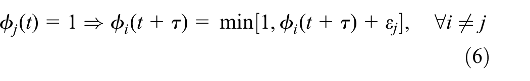
When an oscillator fire at time t, it is

$${\varphi }_j(t)=1\Rightarrow {\varphi }_i(t+\tau )=min[1,{\varphi }_i(t+\tau )+{\epsilon }_j],\forall i\ne j$$

(6)

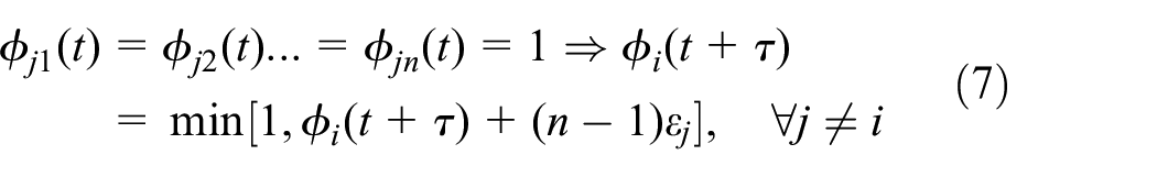
if n ≥ 2 oscillators fire at time t simultaneously, it is

$$\begin{array}{c}\multicolumn{1}{c}{{\varphi }_{j1}(t)={\varphi }_{j2}(t)...={\varphi }_{\mathrm{jn}}(t)=1\Rightarrow {\varphi }_i(t+\tau )}\\ \multicolumn{1}{c}{=min[1,{\varphi }_i(t+\tau )+(n-1){\epsilon }_j],\forall j\ne i}\end{array}$$

(7)

The delay of the proposed model is a real and intuitive of signal condition transmission, that is, the transmission delay is the time spent from the “fire” packets generation to their arrival at the sink, ³⁶ and pulse transmission relates to the times between the receipt of the pulse by the transmitting oscillator in the neighbor and the transmission of a pulse. ³⁷

Oscillator dynamics

Oscillator dynamics with coupled delays were given in different ways. Combining the overview in section “Delayed linear PCOs model,” we can summarize the process of the oscillator dynamics in the Algorithm (Oscillator dynamics).

Algorithm. Oscillator dynamics.

Require: ϕ← random (0,1)     % Initialize phase ϕ Require: $\tau \in (0,1)$ Require:ε > 0 1: procedure Oscillator 2: ϕ←ϕ+Δϕ     % Linear increase of phase 3: ifΔϕ < τ then     % If phase is inside the delay period 4: Δϕ←Δϕ + Δt 5: end if 6: ifΔϕ > τ then     % If phase is outside the delay period 7: ϕ←ϕ + ε 8: ifϕ ≥ 1 then     % If phase is outside the threshold period 9: ϕ← 1 & ε & ϕ← 0     % produce coupling factor ε of the “fire” state 10: end if 11: end if 12: end procedure

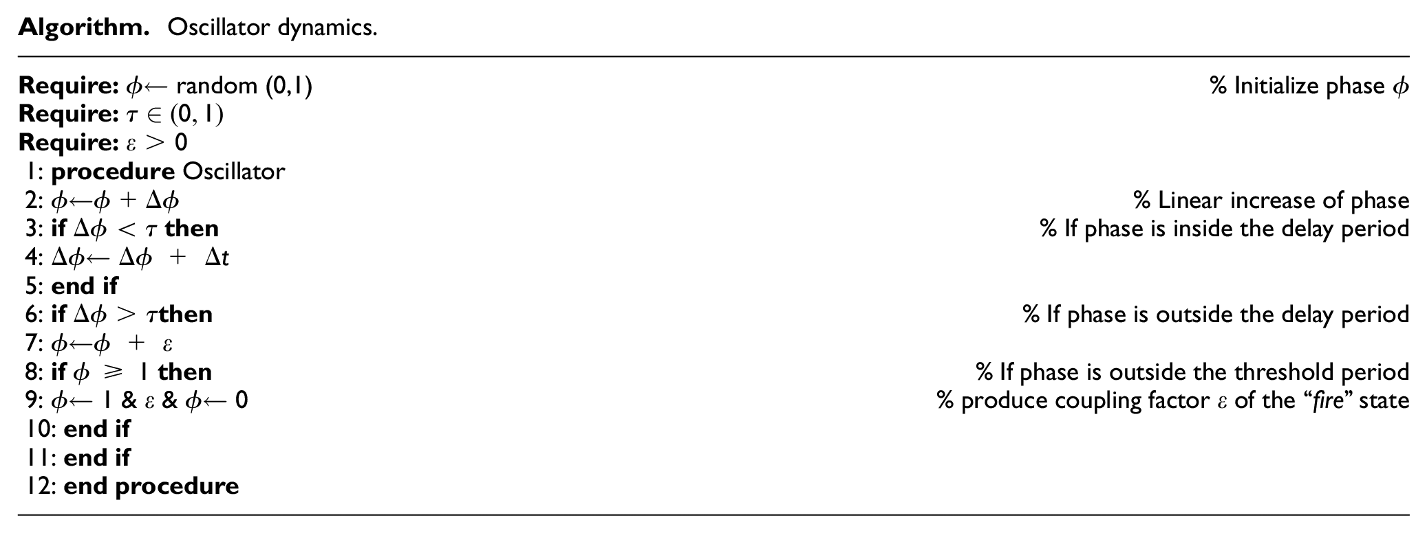
The dynamics are presented in the linear state change function with the value of the phase $\varphi \in (0,1)$ , which is randomly initialized. In each control cycle, the procedure oscillator is executed. ϕ is advanced by Δϕ (Line 2) at the beginning of each cycle. The “fire” condition occurs when the threshold ϕ = 1 is reached (Lines 8–10). The oscillator then begins another loop by resetting the phase to 0 and generating the coupling factor ε to signal the node of the adjacent node for a delay time of Δϕ > τ. Another node can perceive the node. In that case, the neighboring nodes will be gradually updating their stage by a factor ε (Lines 6 and 7). Note that, if Δϕ < τ, the neighboring node will be fired after Δt (Lines 3–5).

Network topology and preliminaries

In sensor networks, there are many kinds of network topologies, such as star network, mesh network, and hybrid network (layered network). For indoor environments, such as coal mines, underground pipe corridors, and building office spaces, there are many intricate roadways or corridors. Due to the low cost, scalability, and topology variability of WSNs, it is not the best choice to deploy large-scale all-to-all communication network sensors. ³⁸ Therefore, we study synchronization in a ring-chain hybrid network topology with nearest neighbor communication (Figure 3). Each node only communicates with its neighbor nodes and sends pulse signals in the excitation state. When the signal passes through the delay, the neighbor nodes are excited and coupled to change the phase of the current time.

Figure 3.

The chain-ring hybrid network topology.

The pulse signal in the ring-chain hybrid network can only excite neighboring nodes, and the excitation is not instantaneous. Therefore, in the process of synchronization of the nearest neighbor network, a huge number of excitations coupling signals are required to excite the neighbors of each node, and the excitation has a delay.

In the nearest neighbor coupling network, since we have no way to determine the position of the delay and pulse signal, the synchronization process of the linear model considering the delay is more complicated. In this article, synchronization can be defined as:

Definition 1

If there are delay τ and time t₀ such that ϕ_i(t₀) = ϕ_j(t₀) for all t₀ ≥ τ, then the oscillator i and j shall finish the entire synchronization process.

Definition 2

If there exist delay τ and time t₀ such that ϕ₁(t₀) = ϕ₂(t₀) = …= ϕ_n(t₀) for all t₀ ≥ τ, then the oscillators can achieve complete synchronization.

In order to grasp the position of the pulse signal when it is not passing through the delay, we use the symbol D_i(t) and D_j(t) ³⁹ to determine the position of the pulse signal

$$D_i(t)=\{\eta =t\prime +\tau -t|t\prime \in T_i\cap [t-\tau ,t)\},i=1...,n,t>0$$

(8)

$$D_j(t)=\{\eta =t\prime +\tau -t|t\prime \in T_j\cap [t-\tau ,t)\},j=1...,n,t>0$$

(9)

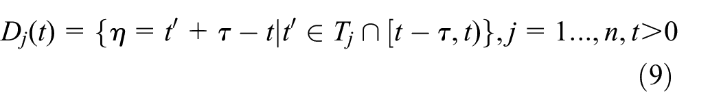
This can be used to obtain the arrival time after the delay of the pulse signal from the ith oscillator.

In a mathematical sense, we can use the firing map h(ϕ) and return map R(ϕ) to explore the development process of oscillators system and the relationship of oscillator phases. ²⁸ To get the synchronization behavior of linear PCOs model with coupling delay, we trace the development of phase differences between oscillators, the total Δϕ_{i, j} is given by

$$\mathrm{\Delta }{\varphi }_{i,j}(t)={\varphi }_j(t)-{\varphi }_i(t)$$

(10)

The firing map h(ϕ) and return map R(ϕ) can be defined as:

Definition 3

Given two oscillators i and j, assuming that at the instant after one firing of i the phase of j is ϕ, the firing map of i about h(ϕ) is defined as the phase of i after the next firing of j.

Definition 4

Given two oscillators i and j, assuming that at the instant after one firing of i the phase of j is ϕ, the return map of j about R(ϕ) is defined as the phase of j after the next firing of i.

Mathematical analysis

We consider two oscillators’ system S as i and j in the linear PCOs model, excitatory coupled with time delay τ. The phase tracking of the system consisting of two oscillators reveals the map of firing and return. The state shift is obtained from the firing map h(ϕ), and the synchronization condition is obtained from the return map R(ϕ), where the address of the pulse signal in the delay is obtained from D_i(t) and D_j(t). The determination of the fixed point for system S is unique, allow the synchronization of the system status over a finite number of variations to be verified.

Our strategy is to (ϕ, ε) space is divided into discrete phase domains I1, I2, and I3

$$\begin{array}{c}I1:\varphi \in [0,\tau )\hfill \\ \multicolumn{1}{c}{I2:\varphi \in [\tau ,1-\tau )}\\ \multicolumn{1}{c}{I3:\varphi \in [1-\tau ,1)}\end{array}$$

The coupling strength is different for each oscillator, which we treat separately to get different h(ϕ) in each of them, these fire map h(ϕ) must be determined the long-term behavior of S.

Both oscillators reached the excited state in a first interval I1, but their pulse signals have not yet reached the other oscillators. Therefore, it is appropriate to determine the outcomes of the two pulses being obtained. The second interval I2, only the pulse signal i, has not reached j. As for the interval I3, oscillator j would reach the threshold before the firing stage of i can be received. Each domain will be divided into smaller areas, and we use consecutive numbers to represent Ex0~Ex6 for excitation coupling, as shown in Table 1∼7.

Table 1.

EX1: 0 ≤ ε < 1−(τ + ϕ) & ϕ∈I1.

Time t	ϕi	Di (t)	ϕj	Dj (t)
t 0	0	{τ}	ϕ	{τ–ϕ}
t0 + (τ–ϕ)	τ–ϕ + εj	{ϕ}		{0}
t0 + τ	τ + εj	{0}	τ + ϕ + εi < 1(*)	∅

h(ϕ) = 1−(ϕ_j–ϕ_i) = 1−[(τ + ϕ + ε_i) − (τ + ε_j)] = 1 − [ϕ + ε_i–ε_j].

Since ϕ_i(τ) = τ + ε_j ≥ τ and ϕ_j(τ) = τ + ϕ + ε_i < 1, h(ϕ) τ such that h: Ex1→I2∪I3.

Table 2.

EX2: 1–(τ + ϕ) ≤ ε ≤ 1−τ & ϕ∈I1.

Time t	ϕi	Di (t)	ϕj	Dj (t)
t 0	0	{τ}	ϕ	{τ–ϕ}
t 0 + (τ–ϕ)	τ–ϕ + εj	{ϕ}	τ	{0}
t 0 + τ	τ + εj < 1(*)	{0}	τ + ϕ + εi = 1	∅
(t0 + τ)+	τ + εj	{0}	1→0	{τ}

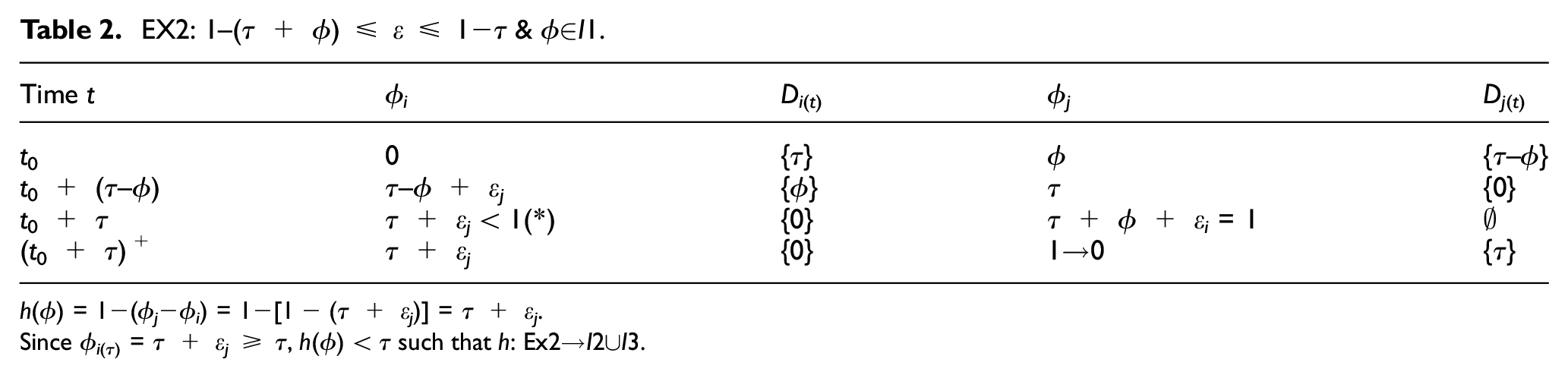
h(ϕ) = 1−(ϕ_j−ϕ_i) = 1−[1 − (τ + ε_j)] = τ + ε_j.

Since ϕ_i(τ) = τ + ε_j ≥ τ, h(ϕ) < τ such that h: Ex2→I2∪I3.

Table 3.

EX3: 1−τ ≤ ε < 1−(τ−ϕ) & ϕ∈I1.

Time t	ϕi	Di (t)	ϕj	Dj (t)
t 0	0	{τ}	ϕ	{τ–ϕ}
t 0 + (τ–ϕ)	τ–ϕ + εj<1(*)	{ϕ}	τ	{0}
t 0 + 1–εj	1→0	{ϕ–[1–(τ–ϕ + εj)]}, {τ}	1 + ϕ–εi = 1	∅
t 0 + τ	τ–1 + εj	{0}, {τ–(τ–1 + εj)}	1→0	∅
(t0 + τ)+	τ–1 + εj	{τ–(τ–1 + εj) = 1–εj}	τ + ϕ + εi = 1	{τ}

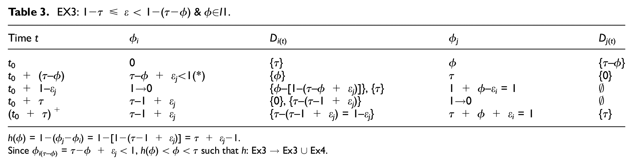
h(ϕ) = 1−(ϕ_j−ϕ_i) = 1−[1−(τ−1 + ε_j)] = τ + ε_j−1.

Since ϕ_i(τ–ϕ) = τ−ϕ + ε_j < 1, h(ϕ) < ϕ < τ such that h: Ex3 → Ex3 ∪ Ex4.

Table 4.

EX4: ε ≥ 1−(τ−ϕ) & ϕ∈I1.

Time t	ϕi	Di (t)	ϕj	Dj (t)
t 0	0	{τ}	ϕ	{τ–ϕ}
t 0 + (τ–ϕ)	τ–ϕ + εj = 1	{ϕ}	τ	{0}
t 0 + (τ–ϕ)+	1→0	{ϕ}, {τ}	τ	∅
t 0 + τ	ϕ	{0}, {τ–ϕ}	τ + ϕ + εi = 1	∅
(t0 + τ)+	ϕ	{0}, {τ–ϕ}	1→0	{τ}

h(ϕ) = 1−(ϕ_j−ϕ_i) = 1−(1−ϕ) = ϕ.

Since h(ϕ) = ϕ, with the same initial conditions only i and j exchanged. This assures that h: Ex4→Ex4.

Table 5.

EX5: ε < 1−(τ + ϕ) & ϕ∈I2.

Time t	ϕi	Di (t)	ϕj	Dj (t)
t 0	0	{τ}	ϕ	∅
t 0 + τ	τ	{0}	τ + ϕ + εi 1(*)	∅

h(ϕ) = 1−(ϕ_j−ϕ_i) = 1−[(τ + ϕ + ε_i)−τ].

Since ϕ_{j (τ)} = τ + ϕ + ε_i < 1, τ<h(ϕ) < 1−τ such that h: Ex5→Ex5∪Ex6.

Table 6.

EX6: ε ≥ 1–(τ + ϕ) & ϕ∈I2.

Time t	ϕi	Di (t)	ϕj	Dj (t)
t 0	0	{τ}	ϕ	∅
t 0 + τ	τ	{0}	τ + ϕ + εi = 1	∅
(t0 + τ)+	τ	{0}	1→0	{τ}

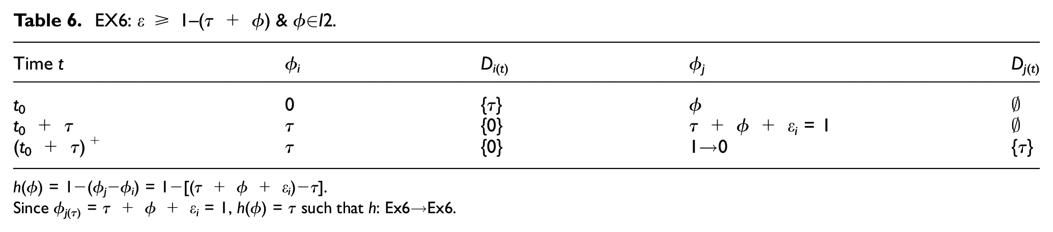
h(ϕ) = 1−(ϕ_j−ϕ_i) = 1−[(τ + ϕ + ε_i)−τ].

Since ϕ_j(τ) = τ + ϕ + ε_i = 1, h(ϕ) = τ such that h: Ex6→Ex6.

Table 7.

EX0: εϕ & ϕ∈I3.

Time t	ϕi	Di (t)	ϕj	Dj (t)
t 0	0	{τ}	ϕ	∅
t 0 + 1–ϕ	1–ϕ	{0}	1	∅
(t0 + 1–ϕ)+	1–ϕ + εj < 1(*)	{τ–(1–ϕ)}	1→0	{0}

h(ϕ) = 1−(ϕ_j−ϕ_i) = 1−[1−(1−ϕ)] = 1−ϕ.

Since 1−τ < ϕ ≤ 1, h(ϕ) < τ such that h: Ex0→I1.

In the linear PCOs coupling delay model, as the case distinctions needed for a comprehensive analysis of the time evolution of the system are very complex, we need to use the tabular form consistently. The related time steps are displayed along with the related oscillator phases. In the lines marked with an asterisk, the rationale for the upper limits of ε can be found.

Since there are stable excitation mappings in the phase tracking of EX5, as shown in Table 8, we will continue to track the phase in both phase changes until we find the regression mapping R(ϕ), and then obtain the synchronization conditional. It is very important to find its unique synchronization from unstable synchronization.

Table 8.

The phase tracking of EX5.

Time t	ϕi	Di (t)	ϕj	Dj (t)
t 0	0	{τ}	ϕ	{τ–ϕ}
t 0 + (τ–ϕ)	τ–ϕ + εj	{ϕ}	τ	{0}
t 0 + τ	τ + εj	{0}	τ + ϕ + εi < 1(*)	∅
t 0 + 1–ϕ–εi	1–ϕ + εj–εi < 1	∅	1→0	{τ}
t 0 + 1–εj	1→0	{τ}	ϕ + εi–εj	{τ–(ϕ + εj–εi)}

The return map R(ϕ) = ϕ + ε_i–ε_j is obtained, and the phase difference from the initial state is ε_i–ε_j, we obtain the synchronization condition can be found in EX5 as coupling strengths satisfying

$${\epsilon }_i\ne {\epsilon }_j$$

(11)

If there is no coupling delay, under the required conditions ε_i≠ε_j, the two coupled oscillators can always achieve synchronization; more importantly, communication and interaction delays are unavoidable and have unfortunate effects on the accuracy of time synchronization. In order to obtain stable synchronization, we need to deeply analyze the oscillator dynamics of the synchronization process.

In practice, each biologically composed system must deal with many delays that seem to limit synchronization process. In the linear PCOs model with coupling delay, the nodes that reach the threshold cannot continuously interact with each other but exchange pulsed signals at certain times. First, we obtain the phase tracking results described above based on an analysis of the coupling strength of the interactions and the coupling delays, as well as the respective pulses of the three regions signal excitation on the phase state of the oscillator. Then, we judge the time of pulse signal excitation through the symbol D_{i, j}(t) to obtain the respective h(ϕ). Finally, we combine these mappings and determine the long-term behavior of system dynamics changes (Figure 4).

Figure 4.

State transition diagram of the oscillator system.

The activity of the system tends to be synchronized in-state shifts at different intervals if satisfying the synchronization condition. However, there are states EX0↔EX1 & EX2 in the dynamics diagram, if this state is a cycle without boundaries, then the system with delays cannot be synchronized. Therefore, we first track the phase of oscillators i and j with delays in the I3 interval, and then with the comparison of the phase changes without delays of the linear PCOs model. The phase of the two oscillators changes in a linear PCOs model without delay, after a complete pulse signal excitation, the firing map h(ϕ) and return map R(ϕ) of system S are obtained (Figure 5(a)). The phase of the two oscillators changes in a linear PCOs model with delay, after a complete pulse signal excitation, the firing map h(ϕ) _delay and return map R(ϕ) _delay of system S are obtained (Figure 5(b)).

Figure 5.

Track the mapping of the two oscillators: (a) without delay and (b) with delay.

By contrast, we find that in the linear PCOs model, the delay causes the pulse signal leading to the emitted state to not stimulate the oscillator fast enough, and in the presence of the delay, the firing map is less ε_j

$$h(\varphi )=1-\varphi +{\epsilon }_j$$

(12)

$$h(\varphi {)}_{\mathrm{delay}}=1-\varphi$$

(13)

The return graph already passes through both delays τ. The pulse signal passes through the delay τ completely, so that the return graph is unchanged in the case

$$R(\varphi )=\varphi +{\epsilon }_i-{\epsilon }_j$$

(14)

$$R(\varphi {)}_{\mathrm{delay}}=\varphi +{\epsilon }_i-{\epsilon }_j$$

(15)

there is a fixed-point R(ϕ) = ϕ₀ while satisfying the synchronization condition

$$\begin{array}{ccc}R(\varphi )<{\varphi }_0\hfill & \mathrm{if}\hfill & {\epsilon }_i<{\epsilon }_j\hfill \\ \multicolumn{1}{c}{R(\varphi )>{\varphi }_0}& \mathrm{if}\hfill & {\epsilon }_i>{\epsilon }_j\hfill \end{array}$$

(16)

Therefore, the fixed point of R(ϕ) is unique, and the system gradually tends to synchronize at the time when ε_i≠ε_j. We can observe that the cycle between the I3 & I2 interval EX0 ↔ EX1 & EX2 is bounded, the state transfer tends to change in the direction of the synchronous state.

Numerical simulations and analysis

In this section, we evaluate the proposed linear PCOs synchronization model with delay by simulations. We confirm the result of two oscillators and multiple oscillators synchronization with time delays by numerical tests. To evaluate and validate the model, we compared the synchronization period of different delays and the sizes of the network and then tested the model on a simulator for the sensor network.

Numerical examples of two oscillators synchronization with delay

To verify that the synchronization can be formed for the linear PCOs model and the theoretical results demonstrated in the preceding parts, we performed detailed numerical tests of the two oscillators synchronization with different delay events.

The synchronization results are shown in Figure 6. The network of two (N = 2) oscillators, whose initialize phase ϕ_i and ϕ_j (ϕ_i≠ϕ_j), with the coupling factor ε_i and ε_j (ε_i≠ε_j). The coupling delays τ were set to τ = 0.1 (Figure 6(a)), τ = 0.3 (Figure 6(b)), τ = 0.6 (Figure 6(c)), and τ = 0.9 (Figure 6(d)), respectively. From the results, we can clearly note that as the amount of time increases, the oscillators would gradually clump into synchronous firing groups. This state can always be maintained because it will eventually achieve synchronization.

Figure 6.

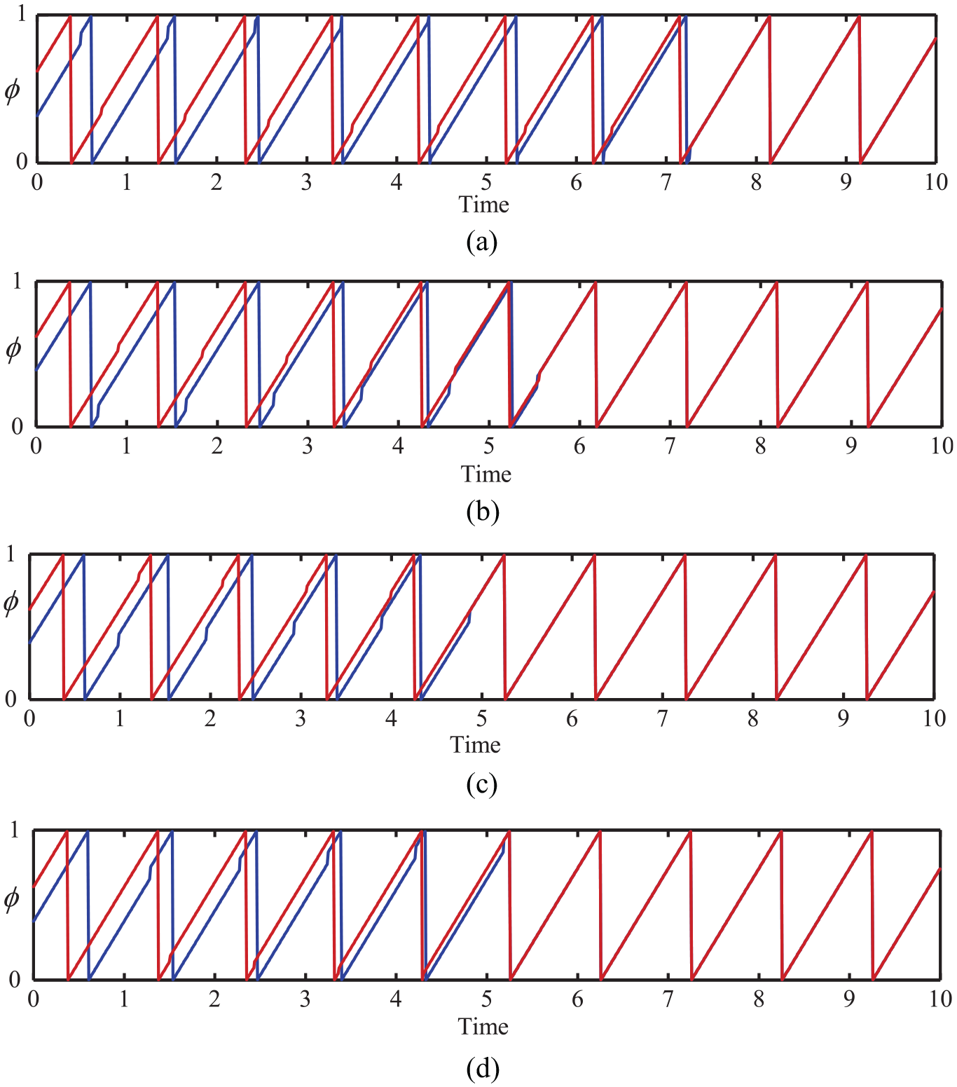
Dynamics of the two oscillators phases ϕ(t) for different values of delay(τ): (a) N = 2, τ = 0.1, ε_i≠ε_j; (b) N = 2, τ = 0.3, ε_i≠ε_j; (c) N = 2, τ = 0.6, ε_i≠ε_j; and (d) N = 2, τ = 0.9, ε_i≠ε_j.

Implementation of multi-oscillators synchronization in a WSN simulation framework

WSNs consist of a few sensor nodes which are wireless. They are equivalent to a swarm of fireflies, using the PCOs guideline to drive accomplices into mating. We put forward the actual realization of the proposed model in the WSNs simulation framework to prove that the proposed multi-oscillators model is useful in solving the time synchronization problem in WSNs. The simulation was introduced in Sinalgo v.0.75.3,^40,41 a platform for test and network validation, building built in Java, Eclipse, and JDK 1.6.

We construct a simple project of “pulseSync” in the sinalgo framework, where each sensor node behaves as an infinite, but delayed repeater of messages it receives. Whenever a node receives a pulse message, it starts a timer to forward the message. A timer is an entity that enables a node to schedule tasks in the future. When the task is due, the timer would notify the node and execute the assigned task. When the timer fires, the node selects its nearest neighbor node with the ID and forwards the message to this node. Then, the timer is reset, and the process is repeated forever. Message transmission delay is described as how long it takes before the message arrives. The delay is determined by the int value of the message and an increment value, specified in the config file. The parameters related to the simulation setup are shown in Table 9.

Table 9.

Initial settings of Sinalgo project.

Parameter	Value
Dimensions	2
Dim x	1000
Dim y	1000
N	25
Transmission range	150
E	(0,1)
T	(0,1)
Can receive while sending	True
Can receive multiple packets in parallel	True
Interference	True
Handle Empty Event Queue	True
JavaCmd	Java

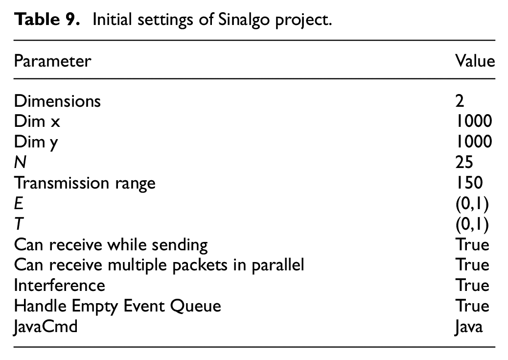
The simulation is composed of the stage of initialization and the stage of simulation. In the simulation stage, it is assumed that the initial phases of 25 oscillators are generated at random at the initialization level, and it is ensured each oscillator is different from the others. The phase of simulation is divided into different cycles. In each cycle, the oscillator with the phase ϕ = 1 is found first, and other oscillators continue to linearly evolve to the firing state. After a period, the phases of the other oscillators are adjusted according to the pulse signal of the fired oscillator, which may contribute to the firing of oscillators. This process remains until no oscillator is fired in the current cycle. We can see from Figure 7 that all the fired oscillators are combined as one single oscillator. Therefore, the oscillators can complete synchronization when there is only one group left and this state can always be maintained.

Figure 7.

Dynamics of the multi-oscillators phases ϕ(t), with N = 25, τ = 0.1, and ε_i≠ε_j.

Then, the evolution of the N = 25 oscillator phases versus the number of cycles is simulated. Each dash in the figure reflects the stage of oscillators in cycles number of the Equal Interval sampling round, and the results are shown in Figure 8. The sampling interval of Figure 8(a) is half a cycle, and the sampling interval of Figure 8(b) is a cycle. From the plot, we can see that as cycles proceed, the number of dashes decreases, and the dash in the figure reflects the stage of a specific oscillator or specific group of oscillators. The oscillators clump into groups gradually. Eventually, the oscillators complete synchronization when there is only one community remaining.

Figure 8.

The phase of multi-oscillators (N = 25) varies with the cycles number: (a) half cycle; (b) a cycle.

Figure 9 displays the number of cycles needed for completing the synchronization process versus oscillators numbers for the initial stage difference ϕ and the coupling delay τ in three intervals I1, I2, and I3(in section “Mathematical analysis”), respectively. To minimize the effect of random characteristics of the ε, we conducted extensive numerical tests of the experiment. From the results, we can conclude that for a certain interval of the phase space (ϕ, τ), more cycles are needed to achieve the synchronization process as oscillators become more in number, since the nearest neighbor network needs more firing nodes and excitation coupling to achieve synchronization, and synchronization convergence speed is slow. In addition, at interval I1, the fixed value of ϕ requires the number of cycles needed to achieve synchronization required cycle than other intervals. This kind of observation is because more and more oscillators’ initial phase and the phase at a certain moment are smaller than the delay in the system. Multiple consecutive pulse signals of more nodes will appear in the delay interval at the same time and there is no guarantee that the phase difference will be reduced. Oscillators are difficult to gather in the synchronous firing groups.

Figure 9.

Number of cycles needed to achieve synchronization versus oscillator numbers.

As a result, the nearest neighbor network requires more firing events and excitation coupling of nodes to achieve synchronization, in order to obtain the best synchronization results in the presence of delays, a good balance must be struck between the initial phase and delay.

Conclusion

In this article, we have studied the time synchronization with communication delay in the nearest neighbor network of distributed sensors, considering the influence factors of practical applications such as message delay, network topology, and computing power of sensor nodes, based on the linear PCOs model of synchronicity achieved by biological systems. In the networks of PCOs with delayed exciting coupling and phase monitoring of the system consisting of two oscillators, we track the development of phase differences between oscillators and discussed the synchronization condition with delay for the oscillator system. From the simulation results, we demonstrated that the system can be synchronized by practically implementing the proposed model in a WSN simulation framework from random initial phase distribution under linear state change functions and nearest neighbor communication. This study provides a new research idea for time synchronization in WSNs consisting of the nearest neighbor communication with delay.