
Abstract
This article mainly uses sparse Global Positioning System trajectory data to identify traffic travel pattern. In this article, the data are preprocessed and the eigenvalues are calculated. Then, the Global Positioning System track points are identified and extracted by walking and non-walking segments. Finally, the three machine learning models of support-vector machine, decision tree, and convolutional neural network are used for comparison experiments. The innovation of this article is to propose a walking and non-walking identification method based on density-based spatial clustering of applications with noise clustering. The method takes into account the continuous state between the geographical distributions, and it has better noise immunity against the influence of external factors. In this process, this article directly achieves better conversion point recognition results through the Global Positioning System track point information, which lays a good foundation for the accuracy of travel pattern recognition. The experimental results of this article show that compared with threshold-based and multi-layer perceptron–based methods, the recognition method based on density-based spatial clustering of applications with noise clustering has the highest accuracy, reaching 82.20%. Then, support-vector machine, decision tree, and convolutional neural network are used for traffic travel pattern recognition. The F1-score of support-vector machine is the highest, reaching 0.84, and the F1-scores of decision tree and convolutional neural network are 0.78 and 0.80, respectively. Finally, the support-vector machine was used for the recognition test to achieve an accuracy of 76.83%.
Keywords
Introduction
Behind the rapid development of urban transportation network, there is a problem of the shortage of transportation resources caused by the urban area and population surge. How to make urban transportation modernization and intelligent development become the focus of the government, citizens, and enterprises. 1 With the revolutionary upgrading of information technology, people have generated a large amount of travel information in their lives, and these information are collected as data, integrated, processed, and analyzed, providing new solutions to solve urban traffic problems, which makes the application of big data technology in traffic field received extensive attention. 2 By processing and analyzing a series of Global Positioning System (GPS) travel data, digital map service providers can help users to provide the best travel plan, and the route recommendation scheme combined with real-time road network traffic conditions can effectively alleviate traffic congestion, morning and evening peaks, and other city traffic problems. Therefore, the travel pattern recognition problem based on GPS trajectory data can benefit multiple parties. However, due to the fact that travel data originate from real life, the accuracy of GPS equipment, the sparseness of data, the differences of travel individuals, and the alternation of multiple travel patterns lead to the complexity of the problem, which makes the problem of far-reaching theoretical research.
For the problem of travel pattern recognition, quite a few scholars have conducted in-depth research on it. Some researchers have used the idea of segmentation between walking and non-walking segments based on transition points, and used conditional random field (CRF) to classify GPS data for travel patterns. 3 Some researchers have analyzed the shortcomings of speed-based single feature classification, and introduced three new eigenvalues of speed change rate, parking rate and direction change rate, and combined with traditional features such as interval maximum speed and interval maximum acceleration to classify travel patterns. 4 Some researchers used the convolutional neural network (CNN) in deep learning 5 and Bayesian network 6 for travel pattern classification. All of the above studies have focused on the improvement of the relevant model of the final travel pattern classification, but there is not much in-depth discussion of the previous trajectory segmentation work.
Combined with the research ideas and deficiencies of the above scholars, the research work of this article is as follows:
First, pre-process GPS trajectory data, including data set field filtering and generation, deduplication, tag correspondence, and data filtering. The base feature values are then calculated based on the unique latitude and longitude of the data set and the time stamp information.
Second, the trajectory segmentation is performed based on the conversion point recognition technique. First, the walking and non-walking points are identified. The threshold method, multi-layer perceptron, and DBSCAN (Density-Based Spatial Clustering of Applications with Noise) clustering are used to compare the performance. Second, the rules to extract and merge the walking and non-walking segments are set, and the GPS track points at the two transitions are marked as the transition points. Finally, the mark transition points are compared with the real transition points, and the recognition result is evaluated by the recall rate and the precision rate.
Third, identify different travel patterns. First, the differences between different travel patterns are analyzed in terms of distance, speed, and acceleration to screen the effective eigenvalues. Second, the eigenvalues are calculated and a series of machine learning models are built to classify the travel patterns. The performance of each model and experiment results are analyzed in the end.
The overall research content of the article is shown in Figure 1. The main difficulties of this research are as follows:
First, the GPS trajectory data collected by the GPS device exist the problem of inaccurate or difficult to correct. Denoising by the corresponding technology will introduce new noise and erase the original trajectory data characteristics. Moreover, the amount of available data in the data set is not large, and there are many walking data in the trajectory data that occur in the community, the park, or even the building, which is difficult to correct.
Second, the trajectory data eigenvalues are calculated based on the Haversine formula in geography to calculate the distance between two given points, where radius is one of the important parameters of the formula. However, the radius of the earth is different at different latitudes, and the calculation of the error will have a great impact on the experiment.
Third, the identification of the transition point is the core of the travel segment division, and the transition point is usually accompanied by a process in which the speed is first decelerated to near zero and then slowly accelerated. This process is very similar to the characteristics of the vehicle waiting for the red light, the arrival and departure of the bus, and the traffic congestion, which is difficult to distinguish correctly.
Fourth, the characteristics of some travel patterns are relatively close. For example, during the period of traffic congestion, the speed of taxi/private car is very close to the speed of bicycles and even walking, and it is difficult to distinguish accurately.

Research content and technical route.
For the above technical difficulties, this article proposes a new solution for the third problem: this article proposes a walking and non-walking recognition method based on DBSCAN clustering. Since the GPS trajectory points in the data set are mostly collected at a fixed frequency, the walking points are denser than the non-walking points, and the DBSCAN clustering considers the continuous state between the geographical distributions, bringing better noise immunity. In the process of identification, this article directly achieves better transition point recognition results through the GPS track point information, which lays a good foundation for the accuracy of travel pattern recognition.
Literature reviews
Travel pattern recognition was first proposed in the United States since the 1960s. In the early days of the study, questionnaires and telephone interviews were the main methods of data collection. Around 2000, the scheme of replacing traditional travel logs with GPS technology to collect travel data was first proposed. Since then, many foreign scholars have proposed characteristic variables such as average speed, maximum speed, maximum acceleration, and travel distance, supplemented by bus route network and site distribution information to identify the travel pattern. With the continuous maturity and application of machine learning, scholars pay more attention to mining GPS data features instead of geographic information system (GIS) information. Models such as decision trees, neural networks, support-vector machines (SVMs), and Bayesian networks have become mainstream algorithm models, and their classification accuracy has been proven to be superior. 3
Travel data can be divided into two types: one is trajectory data based on a single travel pattern and the other is trajectory data mixed by multiple travel patterns. Because the mixed trajectory data contain a variety of traffic characteristics and the transition and stay between different travel patterns, its complexity and variability increase the difficulty of travel pattern recognition. Therefore, the simplification, reconstruction, and semantic mining of trajectory data become the premise and foundation of solving the problem.7,8 For mixed trajectory data, the travel pattern recognition problem is mainly divided into two parts: one is the trajectory segmentation and the other is the pattern recognition. 8 Considering that the state of a single-track point is highly susceptible to the external environment (e.g. traffic congestion, weather, and individual speed differences), the probability of directly identifying a single-track point is higher. Therefore, the longer the trajectory, the more abundant and accurate travel characteristics of the data. 4 In addition, trajectory data derived from real life often contain multiple travel patterns. Therefore, the primary task of trajectory segmentation is to divide the trajectory into sub-sections with uniform travel patterns as accurately as possible, and the number of sub-sections is as small as possible, travel distance and duration are as long as possible. The second step is to perform pattern recognition on the divided sub-sections, mainly by selecting appropriate feature values and using machine learning models for recognition. This article will review four trajectory segmentation methods and pattern recognition problems.
Trajectory segmentation
The core idea of trajectory segmentation is to compute the characteristics of each individual point in the trajectory and to group points with similar features. 9 At present, the commonly used methods for trajectory segmentation are based on unified interval, based on static point, based on GIS data of road network, and based on transition points.
Trajectory segmentation based on unified interval
The unified interval method mostly uses a unified time length, a uniform distance, and a unified GPS track point as a segmentation method. Chang and Newman 10 compared these three trajectory segmentation methods based on uniform interval, and concluded that the performance of these three methods is different in different modes. For example, the unified distance method is more accurate in identifying the taxi/private car mode, and the unified time method is more accurate in recognizing the walking mode. Some researchers also use a fixed period of time as the smallest unit to directly identify the travel pattern of the smallest unit, but after identification, they merge the sections with the same recognition result to improve the accuracy of the segmentation. 11 However, Zheng et al. 12 compared the performance differences between two unified interval segmentation methods (unified duration and uniform distance) and transformation point recognition segmentation methods. They chose the optimal result and transformation point of uniform time length and uniform distance parameter. Compared with the recognition segmentation method, the results show that the unified interval method is inferior to the conversion point recognition segmentation method in almost all evaluation indicators. The main reason is that the unified interval method has a higher probability of including two travel patterns, so it will bring a larger error.
In summary, the shortcomings of the trajectory segmentation method based on unified interval are mainly in the following three aspects. First, the interval selection method of the unified interval method greatly affects the effect of the final trajectory segmentation, its performance is different for different travel modes, and the promotion is poor. Second, the unified interval method needs to select the optimal interval threshold for testing, and the calculation amount is large, and the addition of new data will lead to the change of the optimal threshold and the low adaptability to new data. Third, the unified interval method has a large probability of mixing the GPS track points of multiple travel modes in one interval, so the calculation result of the entire segment feature value does not accurately represent the true characteristics of the travel pattern, and finally leads to the low recognition accuracy.
Trajectory segmentation based on static point
By identifying the point where the speed is significantly smaller than the walking speed, the static point recognition method classifies the point into a non-traveling state, while the non-traveling state has a higher probability that the segment has two independent trajectory segments. 13 Shen 14 used the threshold method to treat a series of speeds as 0 m/s points as non-travel sections, the first point of the section as the end point of the previous trip section, and the last point as the starting point of next trip section. Some research work uses the density-based static point recognition method. When the pause occurs, the GPS trajectory points will be densely located in the same area, thus completing the trajectory segmentation.15,16 Huang et al. 17 further analyzed the commonality of multiple trajectory data staying regions to analyze the repeated behavior of individual travel. Zhou and Yang 18 proposed a new space-time clustering algorithm Adjacent Temporospatial (AT)-DBSCAN to identify the stopping point in the trajectory. The algorithm has a stronger generalization ability for complex problems such as indoor activities and positioning drift.
The activity recognition method is similar to the static point recognition. It is to distinguish the activity and the travel status by connecting the last record point of activity i with the first record point of activity i + 1 to form a travel segment. 19 The advantage of this method is that the actual travel segment can be better extracted from the GPS track points, the non-travel data are removed, and the characteristics of the actual travel mode are more completely and accurately presented. The limitations are mainly as follows. First, the trajectory segmentation method based on the static point can divide the travel chain more effectively, but for the inside of the travel chain, the performance of different travel segment division depends mainly on whether there is obvious stay in the transfer phase. If the traveler walks home immediately after taking the bus, there is no obvious stop in the middle, and the method cannot be effectively divided. Second, the GeoLife GPS Trajectory data set used in this article is affected by the GPS acquisition device, collecting only the GPS track points generated outdoors, and the device will only collect GPS track points if the traveler’s speed or direction changes to a certain threshold.20,21 Therefore, the parking state does not generate GPS track point records in this data set, and the trajectory segmentation based on static point method is not applicable to the data set used in this article.
Trajectory segmentation based on GIS data of road network
Considering that travel data are affected by external factors such as bus arrival, its main features such as speed will be confused with other travel patterns. Therefore, in addition to fully exploiting GPS track information, road network information is also considered by scholars to obtain higher accuracy rate. 22 Especially for public transportation such as bus, subway, and other travel patterns, the geographical location information of bus stations and subway stations provides more powerful support for the identification of the track segment, so some scholars also integrated road network GIS data such as bus lines and subway line data.23,43
The advantage of this method is mainly that the accuracy of track segmentation and travel pattern recognition can be improved to some extent. Especially for buses and subways, if a track has a very high degree of overlap with a bus line or a subway line, then the travel pattern can be basically determined to be a bus or subway. However, the shortcomings of this method are the increase in the amount of data to be processed, the availability of GIS data that can be matched, the scalability of the model, etc. 24 Because this method does more harm than good, although this method is popular in the early days, more scholars tend to explore the characteristics of GPS data itself to complete the travel pattern recognition problem.
Trajectory segmentation based on transition point
The transition point refers to different GPS track points before and after the travel segment. Scholars have adopted different techniques on this issue. Zheng et al. 25 demonstrated that the switching between different travel patterns mostly involves the walking process, so they use the threshold method to pass the two characteristics of velocity and acceleration, differentiate the walking point from the non-walking point, and then merge the trajectory by setting the corresponding rules. The above method has a high dependence on the acquisition frequency of GPS track points due to the extraction and analysis of a large number of point features. Witayangkurn et al. 26 proposed that high-frequency acquisition would consume a lot of battery energy, so in order to be closer to the real-life scene, based on the experiment of Zheng et al., 25 they integrated the speed conversion rate and the number of track points on the subway line as new features, the acceleration characteristics with unstable performance are removed, and the travel mode recognition is performed on the GPS data with low acquisition frequency. Different from identifying the low-speed GPS trajectory points, Yao 27 believes that the travel speed will be repeatedly fluctuated due to external factors such as intersections and traffic congestion, which is similar to signal singularity characteristics; therefore, a wavelet analysis modulus maxima algorithm was introduced to identify the transition points.
The trajectory segmentation method based on transition point recognition has the following advantages. First, the transition point recognition can effectively distinguish the travel segments belonging to different travel patterns, and extract the unique travel segments in the travel pattern, which lays a solid foundation for pattern recognition. Second, compared with the unified interval method, scholar Zheng et al. have confirmed the advantages of the trajectory segmentation method based on the transformation point recognition. Many papers mention the process of the gradual decrease and increase of the switching process of most travel patterns. This feature lays the research direction for the transition point identification. Third, compared with the trajectory segmentation method based on road network GIS data, the trajectory segmentation method based on transition point recognition has weak dependence on data and strong expandability, and greatly reduces the calculation amount, which can achieve faster calculation speed.
At the same time, this method also has some drawbacks: the velocity characteristic near the transition point has a fluctuation process that first decreases and then increases. This process is similar to the characteristics of bus stop station and vehicle waiting signal, 28 so there is a greater likelihood that these points will be mistaken for transition points and will need to be corrected by subsequent steps. However, all the speed-dependent trajectory segmentation methods mentioned above have this defect. Therefore, compared with other trajectory segmentation methods, the trajectory segmentation method based on transition point recognition still has its outstanding advantages.
Travel pattern recognition
Travel pattern recognition is based on the feature values of the extracted trajectory segments to select appropriate machine learning models for classification. In this process, the selection of eigenvalues and models is the most critical.
Speed and acceleration are the two most basic features of pattern recognition, but only the eigenvalues of maximum speed, average speed, and maximum acceleration have proven difficult to distinguish between complex and rich modes of travel. Zheng et al. 4 added new features such as direction change rate, stop rate, and rate of change based on their previous research, and proved these new features have better robustness than the original basic features. Some researchers have proposed acceleration features in the vertical direction to eliminate inter-axis data interference by modulo.29,30 Considering that most travel patterns generally travel in a unobstructed space with good GPS signals, and the GPS signal in the underground space where the subway is located is weak, there may even be no signal inside the tunnel. Therefore, Li et al. 31 have added features related to invalid positioning data to distinguish between subway and other travel patterns. Since the data sets used by various scholars in the experiment process are different, the feature value selection is also greatly dependent on the information provided by the data set.
In terms of model selection, the models used by scholars mainly focus on traditional machine learning models, such as SVM, decision tree, Bayesian network, and random forest. These models mainly rely on the selection of artificial features as the input to complete the classification.13,19,32 The main reasons for using this type of model are: the vast majority of public data set GPS trajectory points are large, but the number of travel segments is small, and it is unable to provide sufficient support for deep learning. However, despite the limited amount of data, some scholars have tried to use the deep learning model to solve the problem of travel model identification. Some experimental comparisons show that if the data volume is increased, the deep learning model has the potential to achieve better recognition results. The method can avoid the disadvantages of long time spent on manual feature selection, high requirements on feature selection for industry experience, and inability to fully display travel characteristics. 23
The content of this article is arranged as follows. The first part introduces the research technology route and innovation point of this article. The second part summarizes the four track segmentation methods and pattern recognition problems. The third part explains the basic concept of travel pattern recognition problem. The fourth part will carry out a series of processing on the data set used in this article. The fifth part will introduce the trajectory segmentation based on transition point method and related experiments. The sixth part will introduce and use three machine learning algorithms for pattern recognition experiments. Finally, the seventh part will summarize the experimental results and make future prospects. The basic concepts of the travel pattern recognition problem are explained in the next part.
Basic concepts of travel pattern recognition
GPS trajectory points
The GPS trajectory point is information that is composed of latitude and longitude coordinates and time stamps, and can describe the spatiotemporal information of the object. 33 The GPS trajectory point is usually represented by Pi. Figure 2 shows an example of a GPS trajectory point. On the right side in Figure 2, P1, P2, …, Pn represent a series of trajectory points, and the left side is an example of the latitude and longitude of the trajectory points and time stamp data.

GPS trajectory point.
Trajectory, travel chain, and start and end points
A trajectory is a segment consisting of a series of consecutive GPS trajectory points
The first GPS track point of the travel chain is the start point, and the last GPS track point of the travel chain is the end point. The start point and the end point are special points in the GPS track point. Figure 3 shows an example of a trajectory, a travel chain, and start points and end points.

Trajectory, travel chain, and start and end points.
Travel segments and transition points
In a complete travel chain, the traveler may use one or more travel modes
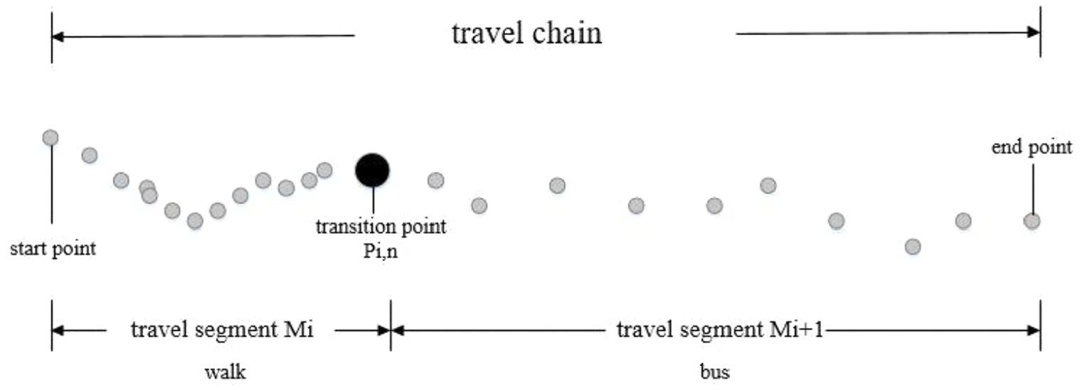
Travel segments and transition points.
Walking and non-walking sections
The walking section indicates that the travel pattern is a walking section of the walk, and the non-walking section indicates that the travel pattern is a travel section other than walking (i.e. bicycle, bus, taxi/private car). The travel pattern recognition mainly includes for identifying the travel segment and identifying the specific travel pattern of the travel segment, so the basis of the travel pattern recognition is the transition point recognition. The general steps are as follows:
First, the GPS track points
Second, for the travel chain, the transition point is marked by the transition point recognition technique. The travel chain before and after the transition point is divided into different travel segments. Finally, the travel segment–related feature values are calculated to identify the travel pattern.
The next part will be a series of pre-processing work on the data used in this article.
Data processing work
Data description
The experimental data in this article are the public data set of the GeoLife GPS Trajectories provided by the GeoLife project from April 2007 to August 2012 by the Microsoft Research Asia. The data set was recorded by 182 volunteers. The data set consists of two parts: the GPS track point and the travel segment information with the travel pattern label. Among the GPS track point data provided by 182 volunteers, 69 recorded the corresponding travel pattern tags. This article selects the data with tags to conduct experiments.
The travel patterns covered by the data set are walking, running, bicycle, bus, taxi/private car, subway, train, airplane, ship, etc. The sample size is shown in Table 1.
Total distance and total duration of each travel pattern.

Due to the small amount of data in some travel patterns (airplane, others), it is impossible to achieve a better recognition effect and is not included in the scope of this study. In addition, because the GPS acquisition equipment is in the state of signal loss in the underground, the way of travel marked as subway is actually light rail, not for the subway. Individual differences in volunteers may cause the light rail to be marked as either train or subway. Considering various factors, the travel patterns within the scope of the study were determined to be walking, bicycles, buses, and taxis/private cars. The data set field characteristics are shown in Tables 2 and 3.
GPS track point data set field characteristics.

GPS: Global Positioning System.
Travel pattern label data set.

Data pre-processing
Data set field filtering and generation
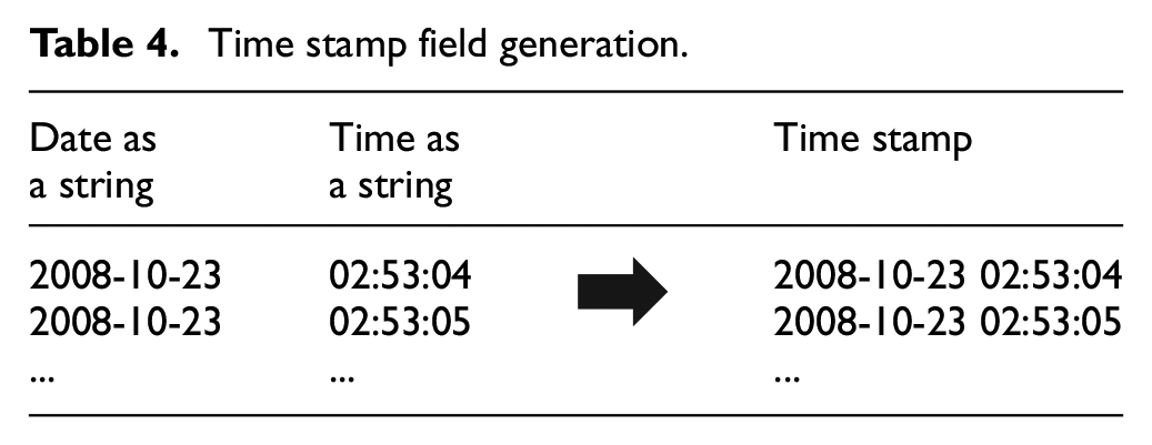
Since the altitude has no effect on the experimental operation, the altitude field in Table 2 is removed. The role of the date field in Table 4 is equivalent to the role of date as a string and time as a string field. To facilitate experimental operation and data understanding, the fields of date as a string and time as a string are named as time stamp field instead of date field.
Time stamp field generation.
After the field is selected, the GPS track point data set data fields are as shown in Table 5.
GPS track point data set data field after field selection.
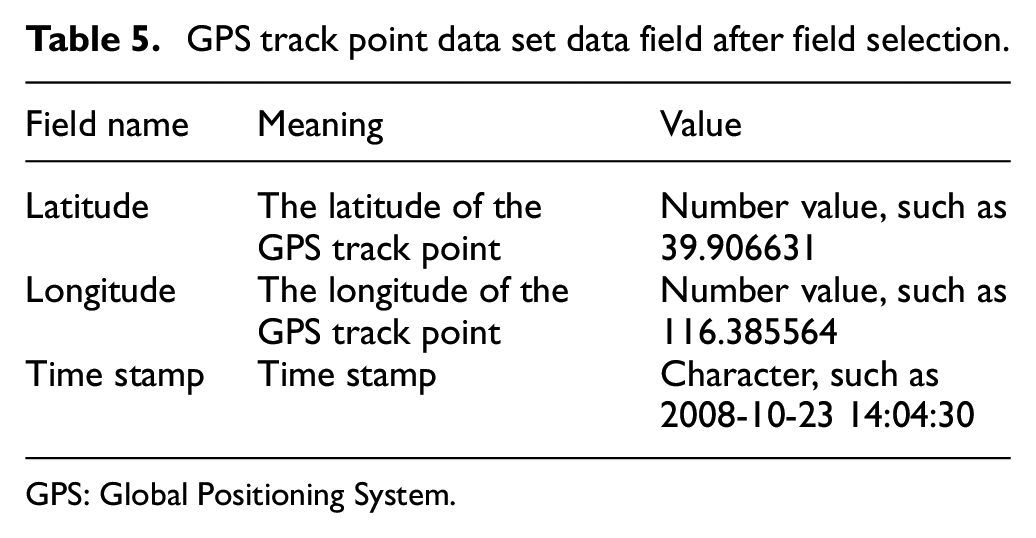
GPS: Global Positioning System.
Data deduplication
Considering that the travel segment label is calibrated by volunteers, many studies using this data set have raised the problem of certain repetitive calibrations, so the travel segment data is deduplicated to obtain the only valid data. 14 In addition, due to the failure of the GPS acquisition device, some GPS track points have data duplication problems. As shown in Table 6, the GPS track point data with the same latitude, longitude, and time stamp are deduplicated.
GPS track point data repetition.

GPS: Global Positioning System.
Label correspondence
The data of Tables 5 and 6 are correspondingly assigned, and the segment tags are assigned to the GPS track points whose time is within the range of the travel segment, thereby obtaining the travel tags corresponding to each GPS data point. At the same time, according to the sequence, the first GPS track point and the last GPS track point in the range of the travel section are, respectively, marked with a start point and an end point. The corresponding data format is shown in Table 7.
Data format after label correspondence.

Data screening
Since the signal quality of the GPS device is affected by the outside world, some GPS data collected will be sparse. Because this part of the GPS data quality problem will cause the two GPS track points to be separated and the distance is far away, only the straight-line distance can be obtained during the calculation. Therefore, this article counts the average GPS sampling rate of each travel segment, and removes the travel segment of a GPS track point after the average GPS sampling rate exceeds 10 s. In addition, because part of the travel segment records is incomplete, the duration is short, and the information covered is too small. In this article, the travel segment with a travel duration of less than 30 s and a GPS track record number (N_log) of less than or equal to 5 is deleted and removed. After screening, the data volume information of each travel pattern is shown in Table 8. The private car and taxi data are small and the travel characteristics are similar, and they are merged into one category.
Data volume of each travel mode after screening.

Basic eigenvalue calculation
In order to extract richer travel characteristics through the latitude, longitude, and time stamp information of GPS track points, the feature values are selected and defined and calculated. The basic eigenvalues include distance between two points, time difference, instantaneous velocity, and instantaneous acceleration. 4 The definition and calculation formula are as follows:
1. Distance between two points
Based on the latitude and longitude information of two adjacent GPS track points, the approximate distance between the two points can be calculated using the Haversine formula, in kilometers 36
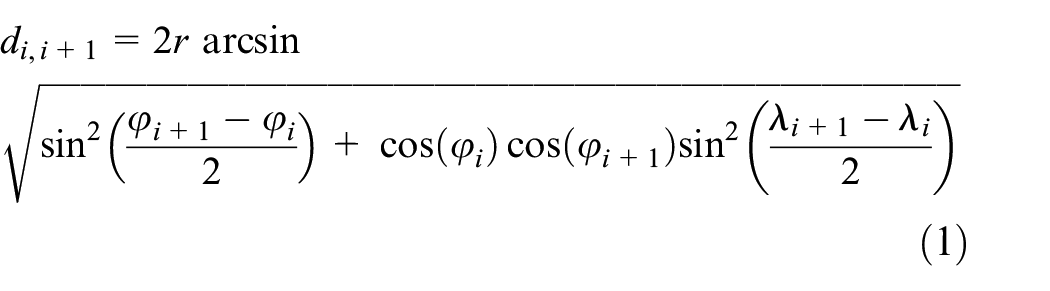
where
2. Time difference
According to the time stamp information of two adjacent GPS track points, the time difference delta t can be calculated and recorded in seconds. The definition formula is as follows

where
3. Instantaneous speed
Instantaneous velocity describes the velocity of an object at a certain time or through a certain position, representing the displacement of the object in an infinitely short time. Since the acquisition time difference between two adjacent GPS track points under normal conditions is very short and mostly concentrated within 5 s, the speed value calculated by formula (3) can be approximated as the instantaneous speed in m/s. It is calculated as follows
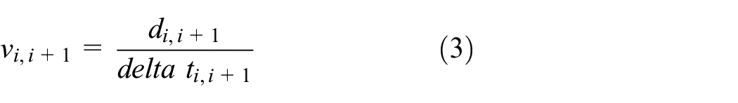
where
4. Instantaneous acceleration
Acceleration is the physical quantity that reflects the speed of the object’s speed change. The instantaneous acceleration describes the degree of change in speed per unit time. When the distance between the two points is short enough, the motion process can be approximated as a uniform acceleration linear motion. The acceleration can be calculated by formula (4), the unit is m/s2, and the definition formula is as follows
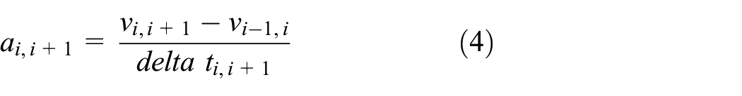
where
5. Direction angle
The direction angle is the angle between the direction of the track from the GPS track point i to the GPS track point i + 1 and the north direction, which can be calculated by equation (5) 37

where
After the data are processed, the next part will describe the track segmentation method based on the conversion point technique used in this article.
Track segmentation method based on transition point recognition
This section will mainly introduce the trajectory segmentation method based on the transition point recognition technology. First, compare the performance of different experimental schemes on the identification of walking and non-walking points. Then, on the basis of the optimal scheme, the walking and non-walking sections are further extracted and corrected, and different extraction and correction rules are compared. Finally, the GPS track points alternated between the two outgoing segments are identified as the transition points, and compared with the real transition points. The track segmentation results are evaluated and discussed by recall rate and precision rate.
Walking and non-walking point identification
This article first calculates the transition probability between different travel patterns. The calculation formula is shown in formula (6)

where
The results are shown in Table 9. More than 85% of the travel pattern transitions experience a walking process, so the first and last GPS track points of the walking segment have a greater likelihood of becoming transition points. In this article, we first distinguish between walking and non-walking points, and then extract the walking and non-walking segments, determine the position of the transition point, and evaluate the results.
Travel pattern transition probability statistical matrix.

Walking and non-walking point identification is the basic work of conversion point identification, and its accuracy has a great influence on subsequent experiments. This article selects three kinds of walking and non-walking point recognition methods: based on threshold setting, based on multi-layer perceptron and based on DBSCAN clustering, and compares their performances.
Walking and non-walking point recognition based on threshold setting
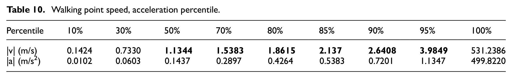
In this article, the absolute values of the speed and acceleration of the walking and non-walking GPS track points are counted. The percentiles are shown in Tables 10 and 11.
Walking point speed, acceleration percentile.
Non-walking point speed, acceleration percentile.

It can be seen from the above table that the difference in the absolute value distribution of the acceleration between the walking and non-walking points is not significant, but the speed distribution of the two is quite different. Based on the 70% quantile of the walking point of 1.5383 m/s and the non-walking point of 25% of the 1.5777 m/s, it can be seen that the instantaneous speed of 70% of the walking points is less than 1.5383 m/s, and only 25% of the non-walking point instantaneous speed is less than 1.5777 m/s. Therefore, this article sets the speed threshold to distinguish between walking and non-walking points. The bold values in Table 10 and Table 11 show that the value distribution of 50% - 95% quantile of walking point is close to that of 20% - 50% quantile of non-walking point. Therefore, when setting parameters, the speed threshold interval is set as [1,4], and the step size is 0.5.
Walk and non-walking point recognition based on multi-layer perceptron
The principle of multi-layer perceptron is given in Yang. 38 The input of the constructed multi-layer perceptron is the GPS track point with label (walking, non-walking) and the velocity and acceleration characteristics. At the same time, the parameters of the hidden layer, the number of neurons, and the activation function are adjusted. The classification accuracy rate and the loss value are used as evaluation indexes, and finally, the label classification result of the GPS track point is output.
Walking and non-walking point recognition based on DBSCAN clustering
DBSCAN clustering uses homogeneity and completeness as evaluation indicators to achieve the best effect of making the sample distance within the cluster as close as possible and the distance between the clusters as far as possible. The two indicators are calculated as 39


where n is the total number of samples,
The DBSCAN clustering in this article only uses homogeneity as the evaluation index. The main reasons are as follows: most of the GeoLife GPS Trajectory data sets selected in this article collect GPS tracking points with a fixed frequency of 1–5 s. Therefore, the walking point presents a denser distribution than the non-walking point. Figure 5 is a trajectory diagram of a travel chain that is converted into a driving. It can be seen that the GPS trajectory distribution of the walking section is much denser than that of the non-walking section. The distribution characteristics of GPS track points near the transition point have undergone significant changes. Therefore, this article borrows the density-based characteristics of DBSCAN clustering, and distinguishes between walking and non-walking points, which is essentially a two-class problem.

Visualization of GPS trajectories in walking and non-walking sections.
The output of the binary classification problem should be the points (i.e. walking points) and the noise points (i.e. non-walking points) that are clustered in the cluster. Therefore, no matter how many clusters are formed in the DBSCAN cluster, the actual labels of the points in the cluster are actually consistent. The completeness represents whether the data points with the actual label consistency are divided into a cluster by DBSCAN clustering. In this problem, the walking points do not need to be clustered in one cluster, so the evaluation index completeness is not applicable in this study. The homogeneity represents whether a cluster formed by DBSCAN clustering only contains the same data points. In this study, the true label of a cluster should be walking, so the homogeneity of the index is in this study is still applicable.
Because DBSCAN clustering based on density-based characteristics to solve the two-category problem, the final result of evaluating its performance is still the accuracy of its classification. Therefore, the classification accuracy rate is used as the main evaluation index, and the homogeneity is used to prove the performance of DBSCAN clustering. 40 The experimental scheme is as follows: the model input is GPS track point data with a label (walk, non-walk), and the adjustable parameter is a distance threshold ε of a certain point field and a threshold MinPts of the number of samples in a certain point field, wherein the range value of ε is [5, 10, 15, 20, 25, 30] and the range of MinPts is [5, 10, 15, 20, 25, 30]. The classification accuracy and homogeneity were used as evaluation indicators. The model output is the DBSCAN clustering result under optimal parameters (−1 is noise, the other is cluster, such as the nth cluster label is n). The noise point label is named as non-walk, and the other cluster point label is named as walk.
Comparison and analysis of experimental results
When the walking and non-walking point identification scheme based on the threshold setting is selected, the experimental results are as follows: when the speed threshold
When using the multi-layer perceptron–based walking and non-walking point identification scheme, the specific experimental scheme is as follows: the multi-layer perceptron is built using the sequential model of Keras. Use the sigmoid as the activation function. Adjustable parameters include the number of hidden layers, the number of neurons in each layer, and the activation function. In order to determine the optimal number of iterations, this article selects the EarlyStopping function in Keras. Taking the validation set loss as the reference, if the validation set loss is not improved within two iterations, the training is stopped, and the improvement amount <0.0001 is no improvement. The structure of each model and its performance are shown in Table 12.
Classification accuracy of each model structure of multi-layer perceptron.
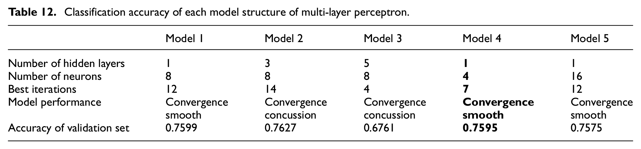
Through comprehensive comparison, it can be found that in the models 1, 2, and 3, as the number of hidden layers increases, the performance of the model shows a decreasing trend. Considering that the input of the problem itself is relatively simple, increasing the network depth will affect the performance of the model. Therefore, a multi-layer perceptron with a hidden layer number of 1 is more suitable for this problem. By comparing the models 1, 4, and 5, it can be seen that the change in the number of neurons generally has little effect on the performance of the model. Considering comprehensively, in order to reduce the complexity of the model and speed up the training of the model, the model with the best performance is model 4 (as shown with bold values in Table 12).
When using the walking and non-walking point identification scheme based on DBSCAN clustering, the accuracy of each parameter and its corresponding classification result are shown in Table 13.
ϵ ∈ [5, 30], MinPts ∈ [5, 30], step = 5, DBSCAN clustering accuracy.

It can be seen from Table 13 that when ε is gradually increased, MinPts can only continue to maintain a superior recognition result as it becomes larger. If ε increases and MinPts does not change, then more points are identified as noise (i.e. non-walking points). It can be seen from the bold values in Table 13 that the optimal combination of the two relations basically appears at the diagonal of Table 14, that is, ϵ = MinPts, and as ε increases, the correct rate of DBSCAN clustering also increases. Therefore, this article further sets up a new parameter pool (ϵ = MinPts ∈ [50,300], step = 50) to conduct experiments. When ε = MinPts = 200, the DBSCAN clustering effect is optimal, and the classification accuracy rate reaches 0.822. Taking the path chain of Figure 5 as an example under this parameter, the visualization result after DBSCAN clustering is shown in Figure 6. The color point in the figure is the cluster formed by the DBSCAN algorithm (i.e. the walking point), and the gray point is the noise point (i.e. non-walking point).
Example of walking and non-walking point identification output data based on DBSCAN clustering.

DBSCAN: density-based spatial clustering of applications with noise.

Visualization of GPS trajectory in walking and non-walking sections after DBSCAN clustering.
It can be seen from Figure 6 that the DBSCAN algorithm performs better in the walking and non-walking point classification of this travel chain, and only a small number of clusters (i.e. walking points) appear in the non-walking section, which may be due to other external environments such as traffic lights intersections, road congestion, and other reasons. However, only a few points in the walking segment are identified as noise points (i.e. non-walking points), and a plurality of clusters can be found in a walking section. The reason may be that the signal of the GPS mobile phone device is temporarily missing, so that the distance between the two points is large. It is also possible that there are partially adjacent walking GPS track points due to the large instantaneous velocity, resulting in a distance between the two points exceeding the threshold of the current parameter.
The final experimental results of the three experimental schemes are as follows: the optimal parameter based on the threshold scheme is
Compared with DBSCAN clustering, the threshold accuracy and multi-layer perceptron classification accuracy are lower, probably because it depends only on the instantaneous velocity or instantaneous acceleration characteristics, and the two calculations are affected by the radius of the earth in the Haversine formula. The return value itself is in km, so it is easy to cause errors of 10 m or even 100 m. However, the GPS track point has drift and deviation caused by the low precision of the acquisition equipment, and the intermediate calculation further expands the error, which affects the classification accuracy. In addition, these two methods classify each GPS track point as an independent individual and are therefore more susceptible to external factors. The DBSCAN clustering takes into account the number of trajectory points that satisfy the condition, and considers the continuous state between geographical distributions, so it has better anti-noise effect on external factors.
Therefore, in this article, the walking and non-walking point identification scheme based on DBSCAN clustering is selected, and the distance interval delta d and time difference delta t of each GPS track point from its next GPS track point are calculated. The final output data are shown in Table 14, where the predict mode field is the travel pattern identified by the DBSCAN cluster, and the predict result is whether the recognition result is correct.
After completing the walking and non-walking recognition of the track points, the walking and non-walking sections will be extracted below.
Walking and non-walking section extraction
Based on the above-mentioned walking point and non-walking point recognition results, this article extracts the walking and non-walking sections by means of merging and correction, identifies the transition point, and evaluates the recognition result by recall rate and accuracy. If the time difference between the identified transition point and the actual transition point is within 2 min, the recognition result is considered correct.
GPS track point combination
If the GPS track points n − i,…, n,…, n + i are the same in the predict mode field in the walking point and non-walking point identification, the first GPS track point n − i is used as the start point, and the last GPS track point is n + i is used as the end point. The time stamp and latitude and longitude information of the start point termination point are also separately recorded, and the section is assigned a walk or non-walk. In the merging process, if the predict mode values of the GPS track points i and i + 1 are the same, but the delta t field of the point i takes a value greater than 20 min, it is still divided into two segments, with i as the end point of the first travel segment and i + 1 as the start point of the second travel segment. The merge process is shown in Figure 7.

GPS track point merge flowchart.
During the merging process, the number of GPS trajectory points (N_log), total duration (duration), and total distance (distance) in each interval are counted. The combined data are shown in Table 15, where the start latitude, start longitude, end latitude, and end longitude fields are replaced by ellipsis because of limited display space.
Example of output data after GPS track point combination.

GPS: Global Positioning System.
Travel segment consolidation and correction
After the first merger, the duration and distance of the travel section are short, which is quite different from the actual travel distance. Taking Table 15 as an example, the first non-walking segment contains only one GPS track point, and both duration and distance are 0. This is due to the misjudgment of some points during the recognition of the walking point and the non-walking point. Therefore, this article further sets rules to merge and correct these shorter segments.
By selecting small sample data, this article designs and compares the following three experimental schemes to merge the sections whose distance is less than or equal to the threshold C_distance, and the delta t from the next trip section is less than 20 min:
Select the section label with the longest distance in the interval as the entire segment label. The accuracy rate is 77.35%.
Compare the total length of the walk section and the non-walk section distance in the interval, and take the larger one as the entire segment label. The accuracy rate is 78.73%.
Compare the number of walking and non-walk GPS track points in the interval (i.e. N_log), and take the larger one as the entire segment label. The accuracy rate is 80.21%.
Comparing the three schemes and the experimental results, it can be found that the experimental results of the scheme 3 are optimal. In the results of Experiments 1 and 2, most of the misidentified travel segments were actually labeled as walk, but were predicted to be non-walk after the merge. The result may be that the travel speed of the non-walk segment is faster, so the distance traveled over the same time is longer. If the actual label of a travel section is walk, which covers a small section consisting of some faster speed points, in the first and second schemes with the driving distance (distance) characteristic as the evaluation standard, the label of this section is very likely to be determined as the entire segment label, resulting in misidentification. The third scheme considers the number of walk and non-walk GPS track points in the whole interval, which avoids the disadvantages of non-walking GPS track points and long driving distance, so the experimental results are better.
Therefore, based on the third scheme, the optimal threshold C_distance is selected and the parameter pool is set to [50, 100, 150, 200]. If the transition point identified by the experiment is within 2 min of the neighborhood near the true transition point, the recognition is considered correct. According to this standard, the recall rate and accuracy of transition points are compared under each threshold. The results are shown in Table 16, and the trend is shown in Figure 8.
C_distance ∈ [50, 100, 150, 200], recall rate, and accuracy result of transition points.


C_distance ∈ [50, 100, 150, 200], the trend of transition point recall rate, and accuracy.
Analysis of conversion point recognition results
According to the experimental results in Figure 8, when the segmentation threshold C_distance is gradually increased, the conversion point recall rate shows a slight downward trend, and the accuracy rate is gradually increased. The reason is mainly because when the C_distance threshold is increased, part of the travel segment with a shorter actual travel distance will be merged into other travel segments during the merge process. When the two travel segments are merged as one segment, the transition point also disappears with the merge, so it cannot be recognized, which leads to a decrease in the recall rate. However, as C_distance increases, the recognition rate of the transition point shows a 2% drop when it is increased to 150 m, and its accuracy is 13% higher than when C_distance = 50. This further illustrates that there is only a relatively low proportion of real short-distance travels in the shorter distance segments before the merger and correction, and most of the rest are due to the inaccurate identification of walking and non-walking points. Therefore, it is necessary to correct it by setting the merge rule and the effect is remarkable.
Therefore, this article finally selects C_distance = 150 as the optimal threshold to complete the trajectory segmentation. The trajectory segmentation form after extracting the transition point is shown in Table 17, where the N_log field represents the number of GPS track points in this travel segment.
Data format after completion of track segmentation.

After the trajectory segmentation is completed, three models will be used for travel pattern recognition.
Travel pattern recognition
This section will first explore the intrinsic characteristics of different travel modes to select more distinctive feature values, and improve the accuracy of late travel pattern recognition. Thereafter, this section will compare the differences in the performance of different machine learning models on the GeoLife GPS Trajectory data set to identify four travel patterns: walk, bicycle, bus, and private car.
Analysis of different travel pattern characteristics
In this article, four sections of the travel pattern of walking, bicycle, bus, and private car are selected, and the speed curve along with the driving distance is visualized. The result is shown in Figure 9. The abscissa is the driving distance and the ordinate is instantaneous speed, where the red line represents the average speed within the line segment.
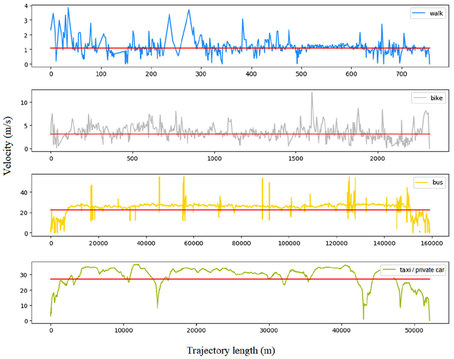
Speed versus travel distance curve in different travel patterns.
It can be seen from Figure 9 that the travel distance and speed distribution of the different travel patterns are quite different. Because the overall speed of walking is slow, the travel distance of the walking section is usually limited by the physical strength of the traveler. The distance of the bicycle is longer than that of the walking. In contrast, buses and private cars have a relatively high speed and can travel a long distance in the same time. Therefore, the distance of the travel segment (trajectory length) is selected as one of the characteristics of different travel patterns.
Second, from the perspective of average speed, there is a significant difference between motor vehicles and non-motor vehicles. Usually, walking < bike < bus < taxi/private car, this conclusion is closer to the actual life. Therefore, this article selects the average instantaneous speed (av) as one of the characteristics of different travel patterns.
From the distribution of instantaneous speed, there are also significant differences between motor vehicles and non-motor vehicles. The stopping frequency of the non-motor vehicle with the speed close to 0 during driving is obviously higher than that of the motor vehicle. Therefore, the stopping rate (SR) is selected as one of the characteristics of different travel patterns. The calculation formula of the SR is shown in formula (9) 4

where
However, the speed is greatly affected by the outside world and the robustness is poor. Therefore, if the different travel modes are distinguished only from the eigenvalue of the average speed, the probability of false positive is higher. As shown in Figure 10, the average speed of the two-segment private car travel section is only about 2 m/s, similar to the performance of the pedestrian travel section on this feature, may be due to long-term slow travel caused by road congestion. However, even though the average speed av characteristics are similar, unlike the ordinary walking section, the instantaneous speed of the private car travel section is still relatively large, exceeding 10 m/s. From the perspective of real life, the instantaneous speed of pedestrians generally cannot match this value. Therefore, in order to more fully describe the speed information of the travel segment, this article also considers the maximum instantaneous speed and selects the three maximum instantaneous speeds as the eigenvalues to reduce the impact of the outliers. In addition, the speed change caused by the external environment is quite different from the speed under normal conditions of the travel pattern, and the motor vehicle is susceptible to such changes due to external factors, so the overall variance of the instantaneous speed is larger than that of the non-motor vehicle. Therefore, this article also selects the instantaneous velocity variance Dv to further comprehensively characterize the velocity characteristics.

Speed curve of private car travel section.
In addition to analyzing the speed characteristics of different travel patterns, this article also analyzes its acceleration characteristics. The results are shown in Figure 11. The abscissa is the travel distance and the ordinate is the instantaneous acceleration, where the red line represents the average acceleration within the travel segment.

Acceleration of different travel patterns with driving distance.
As can be seen from Figure 11, since most of the travel segment acceleration and deceleration processes coexist, it can be found that the average accelerations of the different travel patterns is close to zero. In this article, the instantaneous acceleration is corrected to the absolute value of the instantaneous acceleration, and the analysis is performed again. The corrected result is shown in Figure 12.
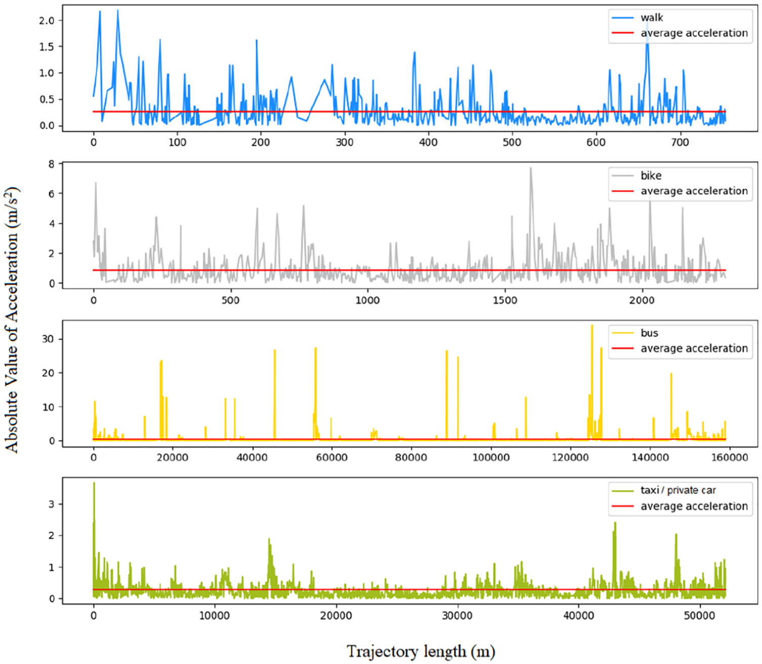
Absolute value curve of acceleration in different travel patterns.
It can be seen from Figure 12 that the instantaneous acceleration of each travel pattern is not obvious from the mean value or the maximum value. Since the four segments are randomly selected and do not have universal representation, in order to confirm the above conjecture, this article calculates the absolute value distribution of instantaneous acceleration of all segments. The result is shown in Figure 13.

Percentage of absolute value distribution of acceleration in different travel patterns.
By observing the percentage distribution of the absolute value of the acceleration in Figure 13, it is further confirmed that different travel patterns behave similarly in terms of acceleration and its absolute value characteristics, and may not be effectively distinguished. Therefore, the maximum value of the absolute value of the acceleration is taken as the undetermined eigenvalue and the experimental comparison is performed.
Feature value selection
The definition and calculation of the basic eigenvalues have been proposed in section “Basic eigenvalue calculation.” Through the analysis of the travel characteristics of different travel patterns in section “Data description,” the eigenvalues listed in Table 18 are also selected to distinguish different travel patterns. Among them, heading change rate (HCR) and velocity change rate (VCR) are obtained by Zheng et al., 12 and the calculation is as shown in formulas (10) and (11).

where HC represents a change in direction,

where VC represents the speed change,
Characteristic value selection and its meaning.
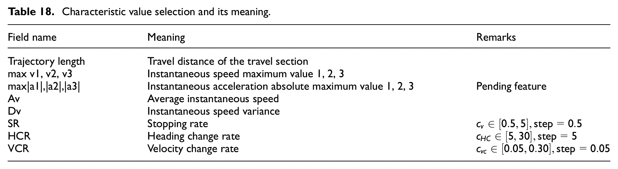
Considering that the calculation formulas of the three eigenvalues of SR, HCR, and VCR need to determine the threshold, this article will first determine the optimal threshold, and then calculate the eigenvalue and construct the model. In order to determine the calculation threshold of the eigenvalue SR, the parameter
Similarly, the HCR calculation method is determined. The test scheme is similar to the above, and the parameters are replaced by
Similarly, the VCR calculation method is determined. The parameters were replaced by
Travel pattern recognition based on machine learning model
SVM-based travel pattern recognition
The principle of SVM is given in Wang et al. 41 The experimental scheme is designed as follows: two inputs are made. The first is the actual travel segment and the extracted feature value of the line segment, and the actual travel segment label, where the feature value is all the feature values mentioned in section “Feature value selection.” The second input is the same as the first, but the feature values max|a1|, |a2|, |a3| are deleted. Then, SVM is constructed for classification, with 70% of the actual travel segment as the training set, 30% of the data as the test set, and the optimal parameters are selected to determine the optimal input. Among them, the adjustable parameters include the SVM kernel function kernel, which ranges from {“rbf,”“poly,”“sigmoid,”“linear”}; SVM built-in parameter C, the value range is [1,10,100]; built-in parameters gamma, the range is [1e−1, 1e−2, 1e−3]; and the degree in the kernel function, which ranges from [1, 3, 5, 7, 9]. The evaluation index is F1-score, and the output of the model is the classification result of the extracted line segment, the model evaluation index, and the operation time.
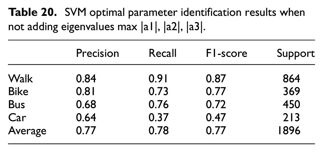
When adding the eigenvalues max|a1|, |a2|, |a3| and not added, the model optimal parameter combination is kernel = “rbf,” C = 10, and gamma = 1e−3. Precision rate, recall rate, and F1-score are shown in Tables 19 and 20. It can be seen from the results of Tables 19 and 20 that although in the above-mentioned travel pattern characteristic analysis part, the discrimination effect of the acceleration-related feature value is not obvious, but in the SVM model, the feature value still plays a certain role. Therefore, these feature values are retained in this article.
SVM optimal parameter identification results when adding eigenvalues max |a1|, |a2|, |a3|.

SVM optimal parameter identification results when not adding eigenvalues max |a1|, |a2|, |a3|.
Travel pattern recognition based on decision tree
The principle of decision trees is given in Bai. 19 Over-fitting problems are more common because decision trees may build overly complex models to approximate the distribution of training sets. Usually, the problem is solved by pruning, setting the minimum number of sample nodes for the leaf nodes, and setting the maximum depth of the decision tree. Therefore, the decision tree model test scheme is set as follows: the input is the actual travel segments, the extracted feature values (the feature values are all the feature values mentioned in section “Feature value selection”), and the actual travel segment labels. Take 70% of the actual travel segments as the training set, 30% of the data as the test set, construct the decision tree model for classification, and select the optimal parameters. The adjustable parameters include the maximum depth of the decision tree (max_depth) and the minimum number of samples of the child node (min_sample_leaf). The evaluation index is F1-score, and the model output is the classification result of the extracted line segment, the model evaluation index, and the operation time. When max_depth = 9 and min_sample_leaf = 10, the model score is the highest. The decision tree model identification results under this parameter are shown in Table 21.
Decision tree model optimal parameter identification results.

Travel pattern recognition based on CNN
Overview of the principle of CNNs
CNN is a widely used deep neural network. 5 It has unique advantages in processing topological data. It can process both one-dimensional time series data and two-dimensional image data. The input of the CNN is a fixed-size multi-dimensional tensor. The model mainly has three types of layers: convolutional layer, pooled layer, and fully connected layer. The overall structure is shown in Figure 14.

CNN network structure.
The convolutional layer consists of a set of learnable filters. By continuously sliding, the filter can learn the local information features of the image. This way, the information can be connected. Each neuron in the convolutional layer output is connected to a small area (receiving field) of the previous layer, where the size of the receiving field is consistent with the filter. The output value of the neuron is calculated by operating the dot product between the parameters of the filter and the entrance of the receiving field. Rotating the same filter over the entire surface of the input body creates a two-dimensional map in the output body, also known as a feature map or activation map. Performing a similar operation on all layers of filters creates several activation maps. Superimposing the feature map of all filters along the depth direction creates a three-dimensional output volume for that layer. The three-dimensional output shape of each convolutional layer is controlled by three hyperparameters specified by the user: the first is the depth of the output volume, which corresponds to the number of filters used for the convolution operation; the second is the step size, which is the number of elements that the filter moves on the input volume at a time; and the third is zero padding, which is the process of adding zero values at the beginning and end of the input volume matrix to control the amount of space in the output.
For travel data, it needs to be converted into approximate image matrix data, and an m × n matrix is formed by the number n of features and the number m of track points in the travel segment. Since CNN requires the input shape of the data to be consistent, the number of track points in different travel segments is usually different. Therefore, this article limits the number of track points for each travel segment to 300 (the median of the number of track points for all track segments) and divides the travel segments for more than 300 track points into multiple input matrices for less than 300 tracks. The travel segment of the point is implemented with a zero-compensation strategy. The input matrix based on features and track points can be expressed by equation (12). Each input matrix uniquely corresponds to a tag matrix, and the tag matrix stores the actual travel tags corresponding to the travel segment

where n = 5 represents the five eigenvalues: v, a, H, HC, and VC.
The purpose of the pooling layer is to achieve spatial and scale invariance, reduce computational complexity, and control overfitting by reducing the dimensionality of each feature map and spatially downsampling the convolutional layer. The largest pooling layer is the most common type of pooling layer, which divides each depth slice of the input volume into non-overlapping vectors, and then selects the maximum value in each sub-vector as the representative value of the vector. The filter size of the largest pooled layer determines the length of the sub-vector (i.e. the number of entries the maximum value should be taken over). Therefore, the depth of the input and output volumes in the pooled layer is the same.
The fully connected layer is the end of the CNN network. Like traditional multi-layer perceptron, each neuron in the fully connected layer is connected to all neurons in the previous layer and is multiplied by unit direction. Except for the last layer, the other layers play the role of extracting features. Subsequently, the advanced features extracted from the first few layers are input to the last layer to perform the classification task, where the softmax activation function is used to generate a probability distribution on the label. The model structure can be adjusted and optimized by increasing and decreasing the number of fully connected layers and the number of neurons per layer. The model finally corrects the weight through backpropagation and finally completes the training process.
Experimental plan and results
In order to adjust the network structure to achieve better experimental results, this article has set up several CNN structures as shown in Table 22. The first parameter of each Conv2D represents the number of filters, the second parameter represents the size of each kernel, and each MaxPooling2D parameter represents the size of pooling windows.
Convolutional neural network model structure scheme.

Comparing models 1, 2, and 3, when the convolution and pooling layer networks are deepened and the number of convolution kernels is increasing, but the full connection layer is not added, the CNN first achieves a superior performance level. However, as the complexity of the model increases, the performance level of the model also declines, which may be caused by the amount of data. Comparing models 1, 4, and 5, when adding the fully connected layer, the performance of the model can be improved, but the number of fully connected layers should not be set too much. Therefore, the model 4 is the optimal model (as shown with bold values in Table 22). The model 4 training results are shown in Figure 15, and the classification results are shown in Table 23.
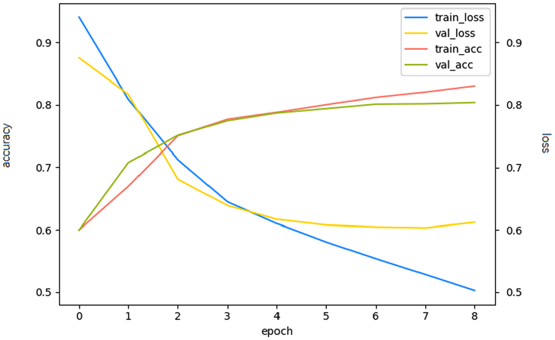
Model 4 training results.
Convolutional neural network under optimal parameter identification results.

Comparison and analysis of experimental results
Comprehensive comparison of three machine learning models, the recognition results under the optimal parameters are as follows: SVM operation takes 26 s, F1-score is 0.84; decision tree operation takes 8 s, F1-score is 0.78; and CNN takes 384 s, F1-score is 0.80. Among the three models, SVM performs best on this problem, while decision tree and CNN perform quite well. The main reason may be that the data volume is small, but the data complexity is relatively high. For decision trees, the model cannot fully learn the connections and rules within the data while preventing overfitting. For the CNN, the complex model structure can better mine the characteristics of the data, but the current data volume is too small for the CNN, and the model cannot be fully trained. If the amount of data can be increased, the performance of the CNN on this issue is still worth looking forward to.
From the perspective of computing time, the decision tree takes the shortest time and the CNN is the longest. SVM achieves a perfect balance of F1-score and computing time under the current data volume. However, if the amount of data is increased, whether the SVM operation time will increase sharply, whether the F1-score performance will be surpassed by the CNN remains to be further verified.
Finally, this article selects the optimal SVM model to classify the extracted travel pattern. Since the transition point recognition is not completely correct, the actual travel pattern corresponding to the extracted line segment may contain more than one. Therefore, this article evaluates the travel pattern recognition result by comparing the correct proportion of GPS track point labels. By calculating the ratio of the track points that match the true results to the total number of track points, the accuracy is 76.83%.
Summary and outlook
Travel pattern recognition based on GPS data can describe user travel rules and features conveniently, efficiently, and accurately. The research results not only can improve the convenience and efficiency of users’ travel but also bring the possibility of profitability to digital map service providers. It will also assist the optimization and upgrading of urban traffic structure and benefit many parties.
This article first summarizes the research status of the field, and on this basis, selects the GeoLife GPS Trajectories public data set released by the Microsoft Research Asia in 2012 as experimental data, and identifies four travel patterns: walking, bicycle, bus, and taxi/private car.
This article mainly completes the trajectory segmentation through the transformation point recognition technology. By counting the data set labels, the experiment found that most of the transfer will have a walking segment, so the start point and the end point of the walking segment have a higher probability of becoming a transition point. In the process of distinguishing between walking and non-walking points, this article proposes a classification method that relates the density-based characteristics of DBSCAN clustering to the density distribution of GPS trajectory points, and obtains a better classification in walking and non-walking point recognition. As a result, it laid a solid foundation for subsequent experiments.
After that, by combining and correcting the travel segments, this article proposes a series of eigenvalues to effectively distinguish different travel patterns, and constructs SVM model, decision tree model, and CNN to compare the performance of different models. The results show that the SVM performs best on this problem, and the F1-score reaches 0.84 under the optimal parameters.
Although this article proposes some improvement schemes for conversion point recognition, there are still many imperfections in the research: for the GPS trajectory data, a more optimized noise reduction processing algorithm is still not found. At the same time, the calculation of the characteristics such as instantaneous velocity is low due to the low sampling frequency of the data, which tends to cause large deviation of the calculation results and affect the final prediction result.
As for the prospect of the work of this article, because the classification accuracy rate is used as the evaluation index in the experiment process, the optimal parameters of DBSCAN clustering are selected by the homogeneity score. The adjustment process needs to be compared according to the actual label, and then selects the optimal value. Therefore, in the future, a parameter adaptive method can be adopted. On one hand, it can be better divided according to different trajectories and individual characteristics of different travelers, and on the other hand, parameter optimization can be realized more efficiently and conveniently. 42
Footnotes
Handling Editor: Lyudmila Mihaylova
Declaration of conflicting interests
The author(s) declared no potential conflicts of interest with respect to the research, authorship, and/or publication of this article.
Funding
The author(s) disclosed receipt of the following financial support for the research, authorship, and/or publication of this article: This research was funded by the National Natural Science Foundation of China (grant no. 61104166).