Energy-efficient chain-based data gathering applied to communicating concrete

Abstract

Wireless Sensor Networks are very convenient to monitor structures or even materials, as in McBIM project (Materials communicating with the Building Information Modeling). This project aims to develop the concept of “communicating concretes,” which are concrete elements embedding wireless sensor networks, for applications dedicated to Structure Health Monitoring in the construction industry. Due to applicative constraints, the topology of the wireless sensor network follows a chain-based structure. Node batteries cannot be replaced or easily recharged, it is crucial to evaluate the energy consumed by each node during the monitoring process. This area has been extensively studied leading to different energy models to evaluate energy consumption for chain-based structures. However, no simple, practical, and analytical network energy models have yet been proposed. Energy evaluation models of periodic data collection for chain-based structures are proposed. These models are compared and evaluated with an Arduino XBee–based platform. Experimental results show the mean prediction error of our models is 5%. Realizing aggregation at nodes significantly reduces energy consumption and avoids hot-spot problem with homogeneous consumptions along the chain. Models give an approximate lifetime of the wireless sensor network and communicating concretes services. They can also be used online by nodes for a self-assessment of their energy consumptions.

Introduction and context

Over the past few decades, the rapid development of chip design made sensing node (SN) ubiquitous. It has been applied vastly in areas from military application, manufacturing traceability, to health monitoring.^1,2 In the framework of Asset Monitoring, the concept of communicating material, proposed in 2009, ³ relates to a material that can communicate with its surrounding environment, and store and process information. Based on this concept, the McBIM (Material communicating with the Building Information Modeling) project, ⁴ funded by the ANR (French National Research Agency), has been coordinated by the CRAN (Research Center for Automatic Control) since 1 January 2018. Two other French research units (LAAS: the laboratory for Analysis and Architecture of Systems; LIB Burgundy Laboratory of Computer Science) and one company (360 Smart Connect/FINAO SAS) are involved.

This project aims to design a “communicating concrete” which is equipped with an embedded wireless sensor network (WSN). This concrete can not only sense its environment (it monitors physical parameters, stores and processes collected data) but can also periodically transmit information to users. Moreover, the McBIM project aims to analyze the usefulness of this concept all along the whole concrete lifecycle, from manufacturing to data exploitation as shown in Figure 1 (communicating concretes are represented as green blocks).

Figure 1.

McBIM communicating concrete lifecycle.

The embedded WSN consists of two kind of nodes as in Figure 2: the SNs for monitoring the surrounding environment and the communicating nodes (CNs) for storing, processing, and transmitting detected information. The SN function is simple and limited. When a SN node has enough energy (provided by harvesting techniques), it just monitors its surrounding physical parameters and transfers data directly to its corresponding CN. The CNs are organized in a network that collects the sensed data from SNs and sends them to a Base Station (BS).

Figure 2.

Diagram of communicating concrete.

In different phases, these elements will be exploited by different users (manufacturers, contractors, or building managers) with their own BIM platform. Besides, the material behaviors may be different over its lifecycle. It is hard to ensure that one data collection protocol can meet all these different requirements over its whole lifetime. This long-term and high-quality service requirement (20 or 30 years) brings challenges related to energy management because it is hard to change batteries in this inaccessible environment. In such a situation, being able to monitor and/or determine the consumption of each node of the network is crucial for its management. As a result, a dedicated energy estimation model can help to provide a rapid reaming energy result to evaluate the nodes’ residual energy. That can be used to adapt the network structure if necessary. In this work, we study how to manage energy for periodic data collection with chained WSN, and our main contributions are as follows:

• A simple, adaptive energy-efficient chain communication scheme for periodic data collection with WSN is proposed (with/without aggregation). Energy efficiency is obtained by reducing number of messages with aggregation and reducing radio activity with a simple sender–receiver synchronization mechanism.

• Analytical energy consumption models (with/without aggregation) for individual node and global chain energy assessment. Predictive models are tested and validated by experimentations (predictions diverge from real measurements by 5%).

• A practical demonstration of the proposed schemes and models (with experimentations and applicative discussion). Models can be used online by nodes to provide an approximate remaining lifetime. According to applicative needs, the difference in energy consumption between a collection with or without aggregation is quantifiable.

The “Assumptions and problem statement” section presents the resource constrained problem related to our communicating concrete. Then “Related works” section introduces the state of the art composed of three complementary parts: energy models of sensor node in WSN, representative chain-based routing protocols, and time synchronization solutions. The concept of communication scheme for McBIM concrete is presented in “Energy consumption models for data collection in chain with or without aggregation” section with its energy consumption estimation model. The relative experiments are shown in the section “Experimental results.” A synthesis and discussion are given in the “Discussion” section. The “Conclusion and future works” section concludes and gives some perspectives for our following work.

Assumptions and problem statement

In the framework of McBIM project, the objective is to solve the maximum lifetime data gathering problem using aggregation (referred to as MLDA in that case) within energy constrained environment. ⁵ In this article, our research issue is to design a dedicated energy estimation model that can provide a previous and rapid reaming energy result. To better understand energy conservation in WSN, Figure 3 depicts the different sensor node elements and their related energy consumptions. The energy consumption of sensor node is mainly composed of three parts: monitoring physical information by sensors, data processing by CPU, and data transmission by radio communication modules.

Figure 3.

Energy conservation of a sensor node.

Some works deal with hardware parts to overcome the resource constrained condition, such as energy harvesting techniques proposed in Kaur et al. ⁶ and Loubet et al.^7,8 Meanwhile, lot of research focus on improving communication efficiency at nodes. ⁹ To do so, some approaches as in-network processing techniques try to minimize the number of generated messages in the network, ¹⁰ while other approaches based on WSN topology help to reduce the gathering path for the source node to the BS. ¹¹ Both are shortly presented hereafter to introduce our problem statement.

To achieve a precise problem statement, we need to clarify the following points with a short literature review: Which communicating structure is adapted for our application? (section “WSN communication structure”), How can aggregation techniques (section “In-network data processing techniques and aggregation functions”) and time synchronization mechanisms (section “Time synchronization problem”) be effective for reducing consumed energy? The problem statement will then be followed by an in-depth review on its related research issues.

WSN communication structure

A short gathering path can help to reduce the transmission cost from source nodes to BS. As a result, many routing protocols for data collection have been proposed since last two decades. Some authors organize nodes in hierarchical structure: chain, tree, or cluster as shown in Figure 4. In a chain-based WSN, nodes transmit information to BS through a line structure.^12,13 In a cluster-based architecture, nodes are grouped into different clusters. Within clusters, one node is elected as a cluster head by a selection algorithm. Cluster leaders aggregate information from its members and transmit aggregated data to BS.^14,15 In a tree-based structure, nodes transmit information along a tree structure as in Tan and Körpeoǧlu ¹⁶ and Han et al. ¹⁷ Network construction in a chain-based structure is easier than in the two others, it is then preferred for small networks. Both tree-based and cluster-based structures are always used for data exploitation of large networks.

Figure 4.

Different routing structures in WSN: (a) cluster-based structure, (b) tree-based structure, and (c) chain-based structure.

In addition to previous mentioned structures, backbone-based structures are also frequently discussed, like Direct Diffusion, Rail Orad, ¹⁸ and Ring Routing. ¹⁹ These protocols define backbone path where data are stored or processed at backbone nodes. Besides, some nature inspired protocols have been studied to extend network lifetime, such as ant colony, ²⁰ gravitational search algorithm, and cuckoo search algorithm.^21,22

In-network data processing techniques and aggregation functions

In-network data processing techniques using both CPU and communication seem to be an attractive solution. ⁹ Instead of directly relaying the received information, the in-network processing techniques use computing ability at intermediary nodes to reduce the number and/or the size of messages, and thus increase the network lifetime.

Aggregation functions are implemented at intermediate nodes or BS to process raw data.^10,23 Basic aggregation functions are simple operations like Average, MAX or MIN, and so on. These operations can reduce transmission cost by losing data accuracy. They cannot be applied to some accuracy required applications. Therefore, data reduction ²⁴ and data compression techniques^25–27 are proposed and widely used in WSN. These techniques aggregate or compress multiple received messages into a big one to reduce message exchanged without losing data. Besides, some data approximation techniques are also widely used.^28,29 They use probabilistic or prediction models at node to reduce communication to the BS.

Time synchronization problem

Although suitable structures and aggregation techniques can reduce transmission cost at node, energy consumption on inactive state should not be ignored. Using sleep mode at node can not only reduce energy consumption but also extend network lifetime. ³⁰ However, the problem that is faced is time synchronization.

In WSN, time synchronization plays an important role. ³¹ Some MAC protocols can handle this synchronization problem. ⁹ These protocols depend on the communication structure. They enable time scheduling. This is especially useful for shifting radio module to sleep mode as often as possible to save energy and extend lifetime.

Problem statement

As the network within one McBIM element is not so large, a simple routing protocol chain-based structure is preferred for periodic building condition monitoring. However, this type of structure is highly impacted by the hot-spot problem. In order to be energy-effective, this work also considers both in-network data aggregation techniques and time synchronization mechanisms to extend the embedded network lifetime.

Given these assumptions, the first step is to be able to evaluate the energy consumption of a chain-based solution with or without aggregation, by designing dedicated energy consumption models. The second one is to compare the energy consumed by chain-based solutions implementing aggregation strategies or not, based on experimentations. These models should be simple and analytical because they will be used online to evaluate the concrete consumption.

To build dedicated models, all the three mentioned MLDA aspects should be taken into account as in Figure 5. In next section, these aspects are detailed, beginning with the different energy consumption models of nodes in WSN, following by related chain-based gathering protocols and time synchronization protocols.

Figure 5.

MLDA problem in WSN.

Related works

The resource constrained limit of WSN has attracted a lot of attention. To estimate network lifetime, energy consumption at nodes has been studied and some energy models have been proposed. As many research works focus on routing protocols to achieving efficient data collections, some algorithms have also been provided to structure the network as a chain. In order to manage the network and to reduce activity of radio interfaces, main WSN synchronization solutions are introduced. Representative energy models, basic chain-based routing protocols, and WSN synchronization mechanisms are thus presented and discussed in this section.

Energy model of sensor node in WSN

Usual “dissipation” model is based on the distance between a transmitter and a receiver and on the size of the data to be transmitted between them ¹⁴ (Figure 6). In this model, the transmission cost $E_{\mathrm{Tx}}$ of a k-bit message with distance d is given by equation (1)

$$E_{\mathrm{Tx}}(k,d)=\{\begin{array}{c}k{E}_{\mathrm{elec}}+k{\in }_{\mathrm{fs}}{d}^2,d<d_0\hfill \\ \multicolumn{1}{c}{k{E}_{\mathrm{elec}}+k{\in }_{\mathrm{mp}}{d}^4,d>d_0}\end{array}$$

(1)

where $E_{\mathrm{elec}}$ is electronics energy; ${\in }_{\mathrm{fs}}\mathrm{and}{\in }_{\mathrm{mp}}$ are amplifier energy for free space and multipath fading, respectively; and d₀ is the distance threshold.

Figure 6.

Radio energy dissipation model.

The receiver energy consumption depends only on message size k: $E_{\mathrm{Rx}}(k)=k{E}_{\mathrm{elec}}$ . This model has been widely used in cluster protocols to estimate node energy consumption.^32,33 However, some authors argue that more realistic states and state transition cost should be taken into consideration.^34,35

Wang et al. ³⁶ propose a hardware-based model: Communication Subsystem Energy Consumption Model. In this model, the main energy cost sub-modules of communication system (receiving module, transmitting module, voltage regulator, crystal oscillator, bias generator, and frequency synthesize) are both considered. Besides transmitting Tx and receiving Rx states, three more states (power off, power down, and power save) are added according to the system state machine. Although transmission modules account for a large part of energy consumption, other components should be considered.

Du et al. ³⁷ present an energy model that considers microcontroller and transceiver. In this model, all states and state transitions for microcontroller and transceiver are considered. Energy consumption is computed by the state power with its time information. An event-trigger based energy model is presented by Zhou et al., ³⁸ which includes processors, RF modules, and sensors. The authors define four different energy models: Processors Energy Model (PEM), Transceiver Energy Model (TEM), Sensor Energy Model (SEM), and Node Energy Model (NEM). In these models, different states of processor and transceiver are both considered, as well as the state transitions. With the proposed event-trigger mechanism as in Figure 7, energy consumption of nodes can then be computed. All mentioned models take one or the main components of node to estimate node and network lifetime.

Figure 7.

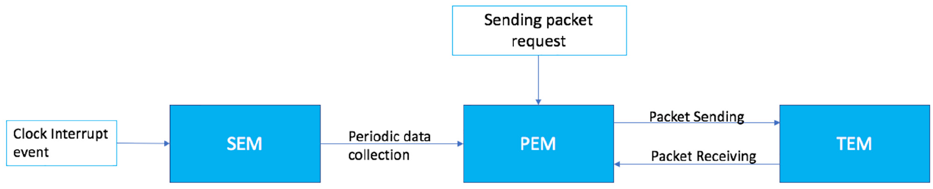
Event-trigger mechanism of NEM.

Other approaches are based on the actual consumption of a sensor node by considering finely the different elements consuming energy in a sensor node.^39,40 A first level of classic decoupling between CPU, sensor, and radio transmitter reveals that the radio transmitter can be responsible for more than 80% of the global consumption (It is true in the majority of cases, except using very complex aggregation functions or energy-intensive sensors like chemical sensors). These models are often used as the decision metric of the construction or organization algorithms of the WSN. They are theoretically true and may give very good approximations for wireless communications.

Energy consumption depends on the routing structure employed to deliver data to the sink. The most representative chain-based routing protocols are presented hereafter.

Chain-based routing protocols

In a chain-based routing protocol, data are transmitted from the furthest node to the BS through a line structure. Data aggregation can be performed at intermediate nodes to reduce data transfer and extend network lifetime.

The first historical chain-based routing protocol using data aggregation is PEGASIS (Power-Efficient Gathering in Sensor Information Systems). ¹² In this protocol, the greedy algorithm is used for chain construction which selects closest neighbor as next hop. In the data collection phase, each node takes turns to act as the leader with the probability i mod N where i is the node number and N is the number of nodes. Data collection begins with one of the end nodes as shown in Figure 8. Data aggregation is performed at all intermediate nodes. This process is then repeated from another side. Once the leader receives all messages, it fuses the data with its own and then transmits them to BS.

Figure 8.

PEGASIS chain-based protocol.

The random leader selection mechanism in PEGASIS balances energy consumption at nodes. Besides, it uses in-network data processing to reduce the amount of transferred data at nodes, and thus extends the network lifetime. However, this long chain structure may have an important impact on the latency. Moreover, the used greedy algorithm only considers the distance between nodes where the remaining energy should also be taken into account.

CRBCC (Chain-Cluster-Based Mixed routing) is a two-layer hierarchical protocol proposed by Zheng and Hu. ⁴¹ Each node is assigned (x, y) coordinates. During the routing, the network is first divided into balanced clusters using y coordinates. In each cluster, the Simulated Annealing (SA) algorithm is performed to form the lowest energy consumption low-level chain. Lower-level chain leaders are elected in the same x coordinates order as in Figure 9. The SA algorithm is then used again for the construction of leader–leader chain. At the end, a top leader is randomly elected to communicate with the BS. In the phase of data transmission, data fusion is also performed in both low-level chain and leader–leader chain. Once the data collection is done, the top leader then fuses all data and transmits them directly to the BS.

Figure 9.

CRBCC protocol.

The route maintenance occurs when a node dies. Each node contacts its neighbors periodically. If it does not receive a reply, it skips the dead node and contacts directly the next one. This two-level chain structure is reconstructed when the percentage of died nodes over the whole network reaches 10%. This protocol combines the advantages of chain-based and cluster-based protocols to overcome the long latency and high reconstruction cost in long chain structure.

To avoid high maintaining cost and reduce the maximum distance of the links for a chain structure, a sub-network chain-based routing protocol (BCBRP for Balanced-Chain-Based Routing Protocol) has been proposed in Ahn et al. ⁴² Compared to the two previous protocols, the chain construction in BCBRP is more complex. It has four phases: diving network, selecting bridge, chain construction with minimum spanning tree (MST), and selecting leader. Data transmission is also through a long chain structure. However, chain reconstruction takes place only in the sub-network which contains the dead node. In this sub-network structure, energy consumption for maintaining the WSN structure is reduced and network lifetime is extended. However, the chain construction is complex, and the single long chain will still cause more delay for data collection.

In these works, authors use the energy radio dissipation model in Liu et al. ²⁶ to construct the network. This model gives a relative and local view of the consumption of a node compared with its neighborhood. Moreover, these protocols assume that all nodes could directly transmit to the BS. Practical WSN deployment show that this assumption is not relevant. Meanwhile, energy cost for inactive state are often ignored in these routing protocol, some solutions for time synchronization are thus presented as follows.

Time synchronization in WSN

Indeed, using sleep mode can save energy at nodes. However, to ensure the communication between nodes with sleep mode, time synchronization problem should be considered. Therefore, some representative time synchronization protocols for WSN are presented and discussed. MAC protocols can be classified into three groups according to synchronization mechanism: sender-based synchronization model, sender–receiver interaction model, and receiver–receiver interaction model. In this section, three representative protocols for each model are presented and discussed.

DMTS (Delay Measurement Time Synchronization) is one of the sender-based synchronization models. ⁴³ For a one-hop network, fewer messages are transmitted. The synchronization message that contains the global time t is broadcasted by the BS. Each child node records the message arrival time t₁ and the time before adjusting its clock t₂. Besides, the delay for transmission t_e can be estimated by the transmission rate of radio module, such as 20 kbps with Mica. Therefore, the delay t_delay is presented as in equation (2). Child nodes then adjust their local times to the global time with measured path delay

$$t_{\mathrm{delay}}=t_e+(t_2-t_1)$$

(2)

This one-hop method can achieve high energy efficiency. However, it is hard to ensure that each node can communicate directly with the BS. Therefore, the authors also discussed the multi-hop version. It uses source levels to identify the distance from the master to another node. Source level of the leader is zero. The synchronization process works as follows: First, a leader selection algorithm is used to select a time master. The leader then broadcasts its time to other nodes. When receiving a time signal, a node will check the level of the time source n. If it is from a source of lower level than itself, it accepts the time and sets its source level to n+ 1. Otherwise, it silently discards the signal. Each node that has been synchronized directly or indirectly with the master broadcasts its time once and only once for a given time sync period. The root node will periodically broadcast its time. At the end, all nodes are synchronized by the multi-hop method.

Reference Broadcast Synchronization (RBS) was proposed by Elson et al. ⁴⁴ Unlike the previous one, this method is based on a receiver–receiver interaction. In this protocol, the reference node (called sender in Figure 10) broadcasts a reference packet to others. When node A receives the packet, it records its local time at T₂₁. Meanwhile, node B also records its local receiving time T₂₂. The nodes can then synchronize by modifying their own time according to the time difference m=T₂₁–T₂₂.

Figure 10.

RBS method.

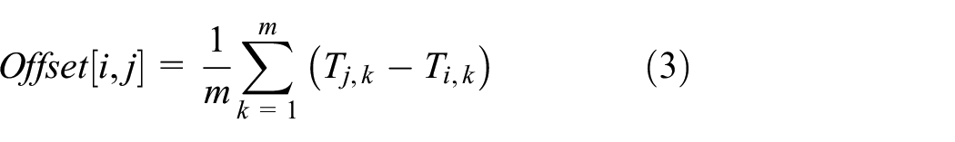
Multi-reference packets are also used to improve the precision of synchronization between two nodes. The transmitter broadcasts m reference packets, any receiver node i can synchronize itself with another receiver j by exchanging all its receiver times T_i,k and T_j,k where k∈m. The offset formula is shown in equation (3). Besides, extension version is also discussed for multi-hop network

$$\mathrm{Offset}[i,j]=\frac{1}{m}\sum _{k=1}^m(T_{j,k}-T_{i,k})$$

(3)

In traditional synchronization protocols, the critical path contains the send time, access time, propagation time, and receive time. However, only the propagation time and receive time are taken into account to avoid the uncertainty of sender. Using this method, each receiver records its message arrival time and then exchange with others to realize the synchronization. By this way, it reduces the send time and access time to improve the accuracy.

Timing-Sync Protocol for Sensor Networks (TPSN) is a sender–receiver interaction method proposed by Ganeriwal et al. ⁴⁵ This protocol is inspired by the NTP (Network Time Protocol) which has been widely used in Internet. Before the synchronization phase, a hierarchical network structure is constructed with a level_discovery message which contains its identity and level to BS.

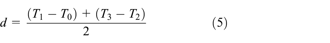
A two-way message exchange method is used for synchronization as shown in Figure 11. Node A first sends a synchronization message that contains its time T₀. Node B records the received time T₁ that is the sum of T₀, α, and d. Here, α represents the clock drift between the two nodes, d is the propagation delay. B then sends back an acknowledgment (ACK) message that contains its level with the three times T₀, T₁, and the sending time of message T₂. Node A records the received time T₃, it can then calculate the clock drift and the propagation delay with the four timestamps as in equations (4) and (5)

$$\alpha =\frac{(T_1-T_0)-(T_3-T_2)}{2}$$

(4)

$$d=\frac{(T_1-T_0)+(T_3-T_2)}{2}$$

(5)

Figure 11.

Synchronization between two nodes in TPSN.

The authors also introduce the notion of real time for error analysis. All packet delays at sender, propagation of messages, and receiver are taken into account. Compared with RBS, this method gives better accuracy. However, its hierarchical structure also increases the energy consumption compared to one-hop solution.

Literature synthesis

The mentioned time synchronization protocols enable time scheduling which provides the chance to use sleep mode at nodes. Besides, some other MAC protocols have been proposed to reduce exchange cost between nodes, like S-MAC, ⁴⁶ R-MAC, ⁴⁷ Tree-MAC, ⁴⁸ and so on. However, these MAC protocols often depend on the communicating structure. In our case, the network within one McBIM element is not so large. Due to the influence of material, the communication distance in concrete is shorter than that in the air. As a consequence, a sender–receiver based TDMA (Time Division Multiple Access) method is more suitable than the two other types. Based on this approach, processes for collection in a chain structure network with or without aggregation are analyzed and models for energy consumptions are constructed in next section.

The well-known chain-based protocols give the basic principles to other works and improvements.^49,50 They use data aggregation techniques to extend network lifetime. PEGASIS extends network lifetime by randomly changing chain leader for each round. However, its long chain structure leads to a high latency. CRBCC divides network into different shorter chains. Its two-level chain architecture achieves a shorter latency than PEGASIS. Unlike both previous protocols, BCBRP reduces the energy cost related to network reconstruction that often occurs in dynamic networks. They both use the mentioned radio consumption model in Heinzelman et al. ¹⁴ They assume that wireless communication interfaces can continuously adapt the power level of the transmission to reach the receiver. In practical applications, the selection of transmission power is almost always a discrete process (even in adaptive methods, thresholds are used).

Distance-based energy models are widely used for the network structuration. Distance seems to be unsuitable for WSNs, especially for distributed algorithms. Because positioning is an intensive-energy task for sensor nodes, most of the time, positioning in WSNs is not possible or energy unrealistic. In our specific case, even if positions of nodes can be known because they can be manually deployed, classical propagation models (free space or multipath models) cannot be applied because sensor nodes are placed in concrete (heterogeneous environment).

In conclusion, energy models always depend on the considered wireless communication technology, they are often impractical for real energy consumption, and especially for the network energy consumption. What we expect is a simple, analytical, and effective energy consumption model which can quickly and accurately estimate the lifetime of nodes in WSN. This remaining lifetime allows to select the appropriate protocol and/or technology for the application. Another usage of this model can be online self-assessment by a node of its consumed energy. We present the development of this model in the following section.

Energy consumption models for data collection in chain with or without aggregation

This section introduces our proposal, that is, analytical energy models for data collection in a chain-based structure. They rely on three hypotheses: (1) node power levels are constant and different depending on the node states, (2) the communication structure is a chain, and (3) the node is sleeping when not sending messages or reading sensor data. We begin with the communication module model. Then, we present a sender–receiver-based data aggregation process expressed via chronograms. Finally, this process helps to define an energy consumption model for chain-based data gathering.

States of the communication module

During data collection, communication takes a large proportion of energy consumption at nodes. The radio communication modules are responsible for sending and receiving data. In this work, four different states are considered for the radio communication module:

• Transmit (Tx): transmitting message to other nodes.

• Receive (Rx): receiving message from other nodes.

• Idle: active but not receiving or transmitting data.

• Sleep: inactive with a low-energy cost.

These modules can shift into different states with some delays as depicted in Figure 12. Transition delays depend on the radio module device and its host microcontroller. Transition costs has been studied by some researchers. ³⁸ Compared with the duration of transmission and data processing at node, these delays are small; we assume that they are negligible in our model. Therefore, to give an approximate WSN lifetime, our model only takes into account the active and inactive states of radio module.

Figure 12.

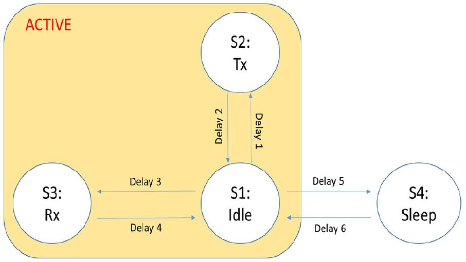
Different states of radio module.

The energy consumption of radio communication module can be simplified with the active and sleep states as in equation (6)

$$\begin{array}{c}E=E_{\mathrm{Tx}}+E_{\mathrm{Rx}}+E_{\mathrm{Idle}}+E_{\mathrm{Sleep}}\hfill \\ =P_{\mathrm{active}}{T}_{\mathrm{active}}+P_{\mathrm{Sleep}}{T}_{\mathrm{Sleep}}\hfill \end{array}$$

(6)

where P_active is the mean power of the three active states (Tx, Rx, Idle); P_sleep is the power expensed in sleep state. T_active and T_sleep are its time intervals, respectively. To estimate energy cost for data collection, it is necessary to compute the intervals for each state. Data collection processes at nodes are detailed in the next section.

Data collection process with/without aggregation

In this section, we present the generic workflow of data collection with or without aggregation at nodes. The data collection in our chain-based network begins from the furthest node. Its workflow is illustrated in Figure 13. At the beginning, communication module is activated to send messages to a parent node. It then waits an ACK message from its parent before letting the communication module enter sleep mode. A delay is used to ensure the reception at the parent node. This node sends its message again if the waiting time exceeds a delay. This node periodically reactivates the communication module for a new transmission process with a period T.

Figure 13.

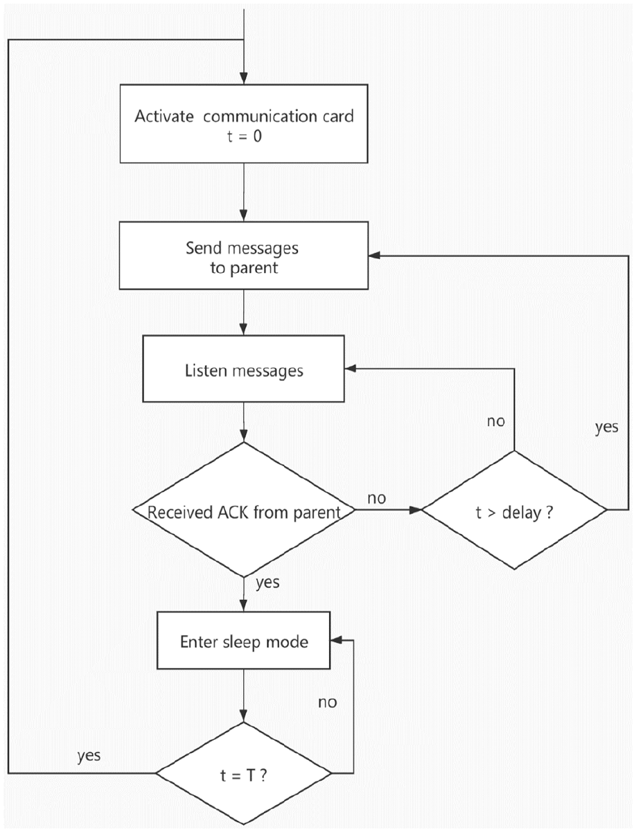
Process at the furthest node.

Data aggregation could be performed at intermediate nodes. Without aggregation, an intermediate node will first transfer all messages from its child. It then sends an ACK message to let its child set its communication module to sleep mode. After finishing the transmission for its child, it then sends its own message to its parent node and waits for an ACK message from it.

Using data aggregation technique can reduce the numbers and sizes of transferred messages and extend node lifetime. The flowchart of intermediate nodes for data collection with aggregation is illustrated in Figure 14. At the beginning, an intermediate node also activates its communication module to listen messages from its child. Instead of directly transmitting received messages from child, it first stores these messages. Once the child node finishes its transmission, it then sends an ACK message back to its child and aggregates received messages with its own one. Only the aggregated message is sent to its parent node. This aggregated message is sent again if the waiting time exceeds a given delay. After receiving ACK from its parent, this node sets its communicating module into sleep mode to save energy. The communication module is reactivated for every iteration, when the node’s local time is up to a scheduled period time. However, to ensure the communication between nodes, the facing challenge is synchronization.

Figure 14.

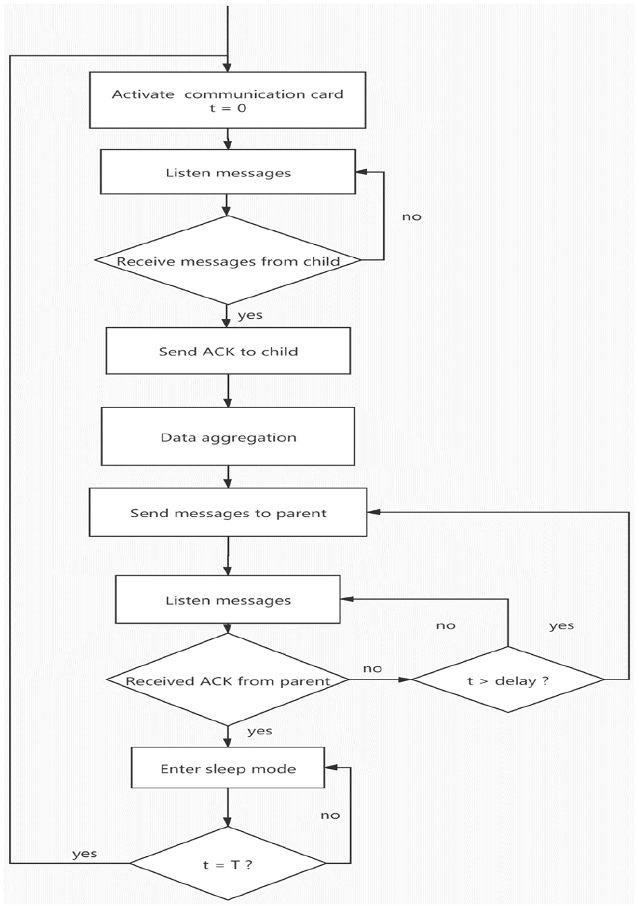
Process at intermediate node.

Synchronization for data collection with/without aggregation

In McBIM project, we suppose that all nodes need to send monitoring data periodically (where period is defined as T). These data are in the same format. Each node can send and receive data from the others. In order to ensure the communication in a chain-based structure, we use a sender–receiver synchronization mechanism. The main idea behinds this mechanism is to achieve a local synchronization between two nodes. Synchronization processes for data collection with or without aggregation are both discussed hereafter.

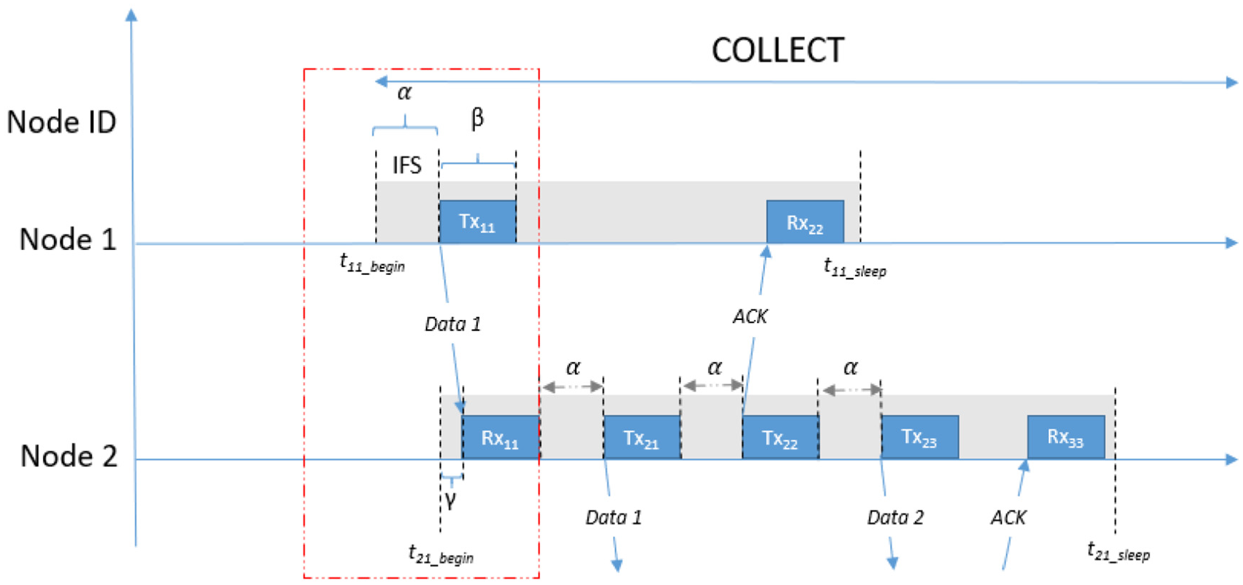
The different processes can be expressed via chronograms. Synchronization is performed during the first iteration period (SYNC). The chronogram on Figure 15 depicts the radio activity of the first two nodes in a chain structure without data aggregation. In chain-based structure, and more generally in wireless environment, any node can receive message from others. To avoid mixing data, inter-frame space (IFS) are generally used in MAC protocols to shift the communication messages. All nodes send messages with a period T. The t_{ij_begin} and t_{ij_sleep} are, respectively, the start time and the time before turning off (sleep mode) radio communication module, where i is the node ID in the WSN, j is the round of iteration. At the beginning of data collection process, all nodes are awake.

Figure 15.

Chronogram of radio module’s activities without aggregation.

In the chronogram, different blocks are used to represent activities of communication modules. The modules are in sending or receiving states with Tx or Rx, respectively. The transmission activities are represented by the node ID and its transfer message number. For example, Tx_ij is the jth message transfer by node i. Meanwhile, the reception activity is presented with the sender ID and data information (like Rx₁₁ is the message 1 from node 1). The modules are in idle state (gray color) when they are active but not sending or receiving data.

Synchronization process begins with the furthest node (here, node 1) at the start time t_{11_begin}. The time before turning off communication module is recorded as t₁₁__sleep after it received ACK message from its parent (node 2). It will turn communication module on for the next iteration at time t=t_{12_begin} where t_{12_begin}–t_{11_begin}=T. The total active duration of the furthest node can then be computed with the recorded start time t_{11_begin} and sleep time t₁₁__sleep.

Unlike the furthest node, the start time for intermediate nodes (here node 2) depends on the previous node. It records the message arrival time of node 1 as start time t_{21_begin}. For data collection without aggregation, it first transmits all messages from its children (node 1) and then sends its own message to its parent (node 3). After receiving ACK message from its parent, it records the time t_{21_sleep} and lets its communicating module enter in sleep mode. For next iteration, it will wake the communication module up a little earlier than its child to ensure the reception of message.

Although using sleep mode can reduce energy consumption at nodes, the hot-spot problem in previous approach is not solved: the closer the node is to the BS, the more energy the node consumes. Therefore, using data aggregation technique could be suitable. It can not only balance energy consumption in WSN but also extend its lifetime. Instead of transmitting all messages from child, intermediate nodes with aggregation send only the aggregated message. The associated chronogram is shown in Figure 16.

Figure 16.

Chronogram of radio module’s activities with aggregation.

The process of the furthest node is the same. However, the intermediate node first stores messages from its child and replies with an ACK message. The received messages are then aggregated with their own message. Only the aggregated message is sent to its parent. In this case, the duration of activity (t_{ij_sleep}–t_{ij_begin}) for communication at each node is less than that without aggregation. Duty cycle at these nodes is reduced, and lifetime is increased.

Energy consumption estimation model for data collection without aggregation

Since lifetime is the most important performance metrics for our application, knowing residual energy of nodes is necessary for energy management. However, it is hard to measure residual energy inside concrete. Building a theoretical energy consumption model could help us to know how the energy is consumed. Therefore, an energy consumption estimation model, based on the mentioned data collection process, is presented hereafter. All used symbols are defined as in Table 1.

Table 1.

Summary of symbols.

Symbols (unit)	Definition
${\mathit{E}}_{\mathit{i}}$ (J)	Communication energy consumption of node i
${\mathit{E}}_{\mathit{total}}$ (J)	Total energy consumption of network
${\mathit{P}}_{\mathit{active}}$ (w)	Power of active state
${\mathit{P}}_{\mathit{Sleep}}$ (w)	Power of sleep state
${\mathit{D}}_{\mathit{i}\_\mathrm{active}}$ (s)	Active duration of node i
${\mathit{D}}_{\mathit{i}\_\mathrm{sleep}}$ (s)	Sleep duration of node i
α (s)	Inter-frame space time
B (s)	Transmission duration
$\mathit{\gamma }$ (s)	Wake up duration
$\mathit{T}$ (s)	Data collection period
N	Chain size
k 1	Constant value $(3\alpha +3\beta )$
k 2	Constant value $(3\alpha +4\beta +\gamma )$
k 3	Constant value $(2\alpha +3\beta +\gamma )$

Energy consumption of nodes depends on power consumption relative to radio state and activity durations. All nodes have fixed power consumption values as assumed in section “Chain-based data collection platform” (these values for our testbed are determined in the next section). Active and sleep modes are the only modes considered in this study, P_active and P_sleep being their respective power consumptions. T is the period of data collection. For building our model and to simplify those variables, we replace the mentioned durations of IFS, transmission Tx, and preparation time for listening incoming messages (between the beginning time and arrival time of child’s message) by some symbols: α, β, and γ (see Figure 17).

Figure 17.

Model parameters explanation.

Let’s begin with node 1. This node first sends its message (β) after the IFS (α). It then waits an ACK from its parent node (node 2). Node 2 first retransfers the received message (α+β) and then replies an ACK message to node 1 (α+β). After receiving the ACK from node 2, node 1 lets its radio module enter sleep mode. Meanwhile, it records the time as sleep time to compute the beginning time for next iteration. In summary, the total duration of node 1 for the data collection phase is 3α+ 3β. This active duration is the minimal time for sending message and getting a reply from parent node in this model. For the intermediate node 2 in a N-node chain structure, its duration of activity consists of three parts: (1) transfer all received messages (α+ 2β), (2) send an ACK message to its child (α+β), and (3) send its own message and wait for an ACK like node 1 (3α+ 3β). Besides, node 2 should wake up a little bit earlier than its previous nodes with γ for the phase of data collection. Therefore, its total active duration is $\beta +2\times (\alpha +\beta )+3\alpha +3\beta +\gamma$ . The process at intermediate nodes are the same. The closer to the BS, the more information needs to be transmitted. The equation can be generalized to the ith node. The duration time of intermediate node i is $\beta +(i-1)\times 2\times (\alpha +\beta )+3\alpha +3\beta +\gamma$ .

For the last node N of the chain, it works as intermediate nodes for the first two steps (the duration is $\beta +(i-1)\times 2\times (\alpha +\beta )$ ). But its last step takes less time, after receiving its message $(\alpha +\beta )$ , the BS will reply with an ACK message $(\alpha +\beta )$ . Therefore, the active duration of node i in a N-node $(N\ge 3)$ chain structure can be expressed in equation (7)

$$\begin{array}{c}{D}_{i\_\mathrm{active}}=\hfill \\ \{\begin{array}{c}3\alpha +3\beta ,\mathrm{when}i=1\hfill \\ \multicolumn{1}{c}{(i-1)\times 2\times (\alpha +\beta )+3\alpha +4\beta +\gamma ,\mathrm{when}2\le i\le n-1}\\ \multicolumn{1}{c}{(i-1)\times 2\times (\alpha +\beta )+2\alpha +3\beta +\gamma ,\mathrm{when}i=n}\end{array}\hfill \end{array}$$

(7)

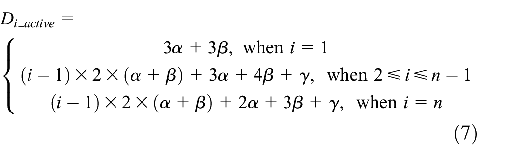
The values of $\alpha ,\beta$ , and $\gamma$ are constant; $3\alpha +3\beta$ , $3\alpha +4\beta +\gamma$ , and $2\alpha +3\beta +\gamma$ can be replaced by constant values k₁, k₂, and k₃. The equation can then be simplified as follows

$$\begin{array}{c}{D}_{i\_\mathrm{active}}=\hfill \\ \{\begin{array}{c}{k}_1,\mathrm{when}i=1\hfill \\ \multicolumn{1}{c}{(i-1)\times 2\times (\alpha +\beta )+k_2,\mathrm{when}2\le i\le n-1}\\ \multicolumn{1}{c}{(i-1)\times 2\times (\alpha +\beta )+k_3,\mathrm{when}i=n}\end{array}\hfill \end{array}$$

The data collection is performed periodically where T is the period. With the duration of activity above, the duration of sleep mode for node i in a N-node chain structure can then be computed as equation (8)

$$D_{i\_\mathrm{sleep}}=T-D_{i\_\mathrm{active}}$$

(8)

In our study, we only consider the active and sleep mode, where the power consumption can be presented by $P_{\mathrm{sleep}}$ and $P_{\mathrm{active}}$ for sleep and active, respectively. Energy consumption per round for node i in N-node chain structure can then be estimated with their duration. The energy consumption $E_i$ of the node i can be calculated as in equation (9)

$$E_i=D_{i\_\mathrm{active}}\times P_{\mathrm{active}}+D_{i\_\mathrm{sleep}}\times P_{\mathrm{sleep}}$$

(9)

Knowing energy consumption at each node, it is then possible to estimate energy cost of whole network for each round. The total cost for one round can be calculated as in equation (10)

$$\begin{array}{c}{E}_{\mathrm{total}}=\sum _{i=1}^n{E}_i=\sum _{i=1}^n(D_{i\_\mathrm{active}}\times P_{\mathrm{active}}+D_{i\_\mathrm{sleep}}\times P_{\mathrm{sleep}})\hfill \\ =\sum _{i=1}^n(D_{i\_\mathrm{active}}\times P_{\mathrm{active}}+(T-D_{i\_\mathrm{active}})\times P_{\mathrm{sleep}})\hfill \\ =\sum _{i=1}^n(D_{i\_\mathrm{active}}\times (P_{\mathrm{active}}-P_{\mathrm{sleep}})+T\times P_{\mathrm{sleep}})\hfill \\ =n\times T\times P_{\mathrm{sleep}}+\sum _{i=1}^n{D}_{i\_\mathrm{active}}\times (P_{\mathrm{active}}-P_{\mathrm{sleep}})\hfill \end{array}$$

(10)

The total active duration is computed as in equation (11)

$$\begin{array}{c}\sum _{i=1}^n{D}_{i\_\mathrm{active}}=D_{1\_\mathrm{active}}+D_{2\_\mathrm{active}}+\cdots +D_{n\_\mathrm{active}}\hfill \\ =k_1+2\times (\alpha +\beta )+k_2+\cdots +\hfill \\ (n-1)\times 2\times (\alpha +\beta )+k_3\hfill \end{array}$$

(11)

Energy consumption model for data collection with aggregation

Similar to section “Six-node chain-based data collection test,” an estimation model is required for this approach. The durations of both activity and sleep are detailed hereafter, as well as the energy consumption estimation model for nodes and the whole network.

In this approach, we also begin with the furthest node. It first sends messages to parent node after duration IFS $(\alpha )$ , and then wait an ACK message. However, intermediate node (node 2) will not retransfer messages as in the approach without aggregation, but first sends an ACK to its child with $(\beta +\alpha )$ . After receiving the ACK message $(\beta )$ , the furthest node shifts its radio module to sleep mode and records its sleep time. Therefore, the total active duration of node 1 is 2α+ 2β.

Duration of activity at intermediate nodes is also in three parts for data collection with aggregation: First, sending an ACK message to its child $(\beta +\alpha +\beta )$ . Second, node 2 aggregates the received message from node 1 with its own message. Third, transmitting the aggregated message and waiting the reply from its parent $(2\alpha +2\beta )$ . Compared with the transmission time, data processing at CPU for the second time is small. Here, we neglect it for building the model. Therefore, the duration of node i for data collection in this approach can be expressed as in equation (12)

$$D_{i\_\mathrm{active}}=\{\begin{array}{c}2\alpha +2\beta ,\mathrm{when}i=1\hfill \\ \multicolumn{1}{c}{3\alpha +4\beta +\gamma ,\mathrm{when}i\ne 1}\end{array}$$

(12)

Similar to the approach without aggregation, each node will set communication module into sleep mode after receiving an ACK message from its parent. Therefore, the duration of sleep for node i can be computed with equation (13). The energy consumption is the most interesting part for us. It can be computed by the same equation (15). The constant $3\alpha +4\beta +\gamma$ can be replaced by k₂. The total active duration can be calculated in equation (13)

$$\begin{array}{c}\sum _{i=1}^n{D}_{i\_\mathrm{active}}=D_{1\_\mathrm{active}}+D_{2\_\mathrm{active}}+\cdots +D_{n\_\mathrm{active}}\hfill \\ =2\alpha +2\beta +3\alpha +4\beta +\gamma +\cdots +3\alpha +4\beta +\gamma \hfill \\ =2\alpha +2\beta +(n-1)\times (3\alpha +4\beta +\gamma )\hfill \\ =2\alpha +2\beta +(n-1)\times k_2\hfill \end{array}$$

(13)

The energy consumption of the whole network can be computed as in equation (14)

$$\begin{array}{c}{E}_{\mathrm{total}}=n\times T\times P_{\mathrm{sleep}}+\sum _{i=1}^n{D}_{i\_\mathrm{active}}\times (P_{\mathrm{active}}-P_{\mathrm{sleep}})\hfill \\ =n\times T\times P_{\mathrm{sleep}}+(2\alpha +2\beta +(n-1)\times k_2)\hfill \\ \times (P_{\mathrm{active}}-P_{\mathrm{sleep}})\hfill \end{array}$$

(14)

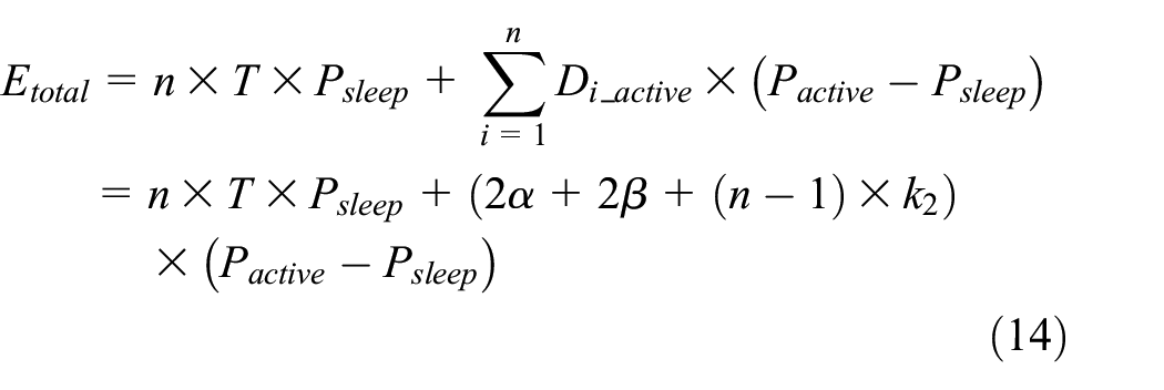
With these mentioned models, we can then estimate energy consumption for data collection with/without aggregation. The size of chain (n), the powers of radio module $(P_{\mathrm{active}},P_{\mathrm{sleep}})$ and data collection period (T) are always fixed values. Due to the difference of active duration, their energy costs are different. A comparative estimation result is shown in Figure 18 where $\alpha$ , $\beta ,\mathrm{and}\gamma$ are fixed at 100, 20, and 10 ms, respectively. When the number of nodes grows, the total active duration increases linearly for data collection with aggregation. This increase is parabolic for data collection without aggregation. The more nodes there are without aggregation, the more obvious the hot-spot phenomenon will be. Therefore, using data aggregation techniques at intermediate nodes may be useful for extending network lifetime. Data collection tests with/without aggregation are presented in next section.

Figure 18.

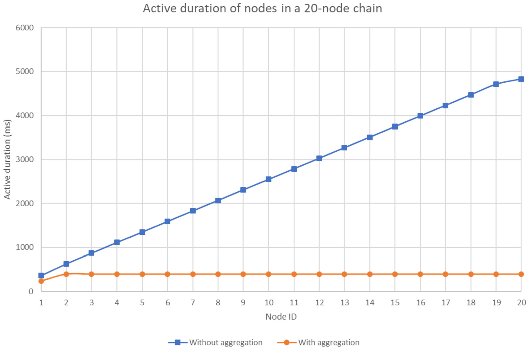
Estimation of active duration for chain-based approach.

Experimental results

We first introduce the materials used for our testbed. We then start with the measurement of power consumption in active and sleep modes. In a second step, energy consumptions with/without aggregation are compared in order to validate the aggregation option with a three-node chain structure. The real energy consumptions of six nodes in chain are recorded and compared to verify the usefulness of our energy estimation model.

Chain-based data collection platform

The chain-based routing structure is suitable for a small network as that within one McBIM element. Before applying these techniques to real concrete, we first build a physical platform with the microprocessor chip Arduino and XBee wireless communication module to verify the usefulness regarding energy saving.

The chain structure design is illustrated in Figure 19. This platform is constituted of microprocessor chips Arduino Uno equipped with the XBee communicating module as shown in Figure 20(c). Each node owns an ID between 1 and N, from the furthest node to the BS. The last node is connected with a PC via a USB cable that can not only transfer data but also provide the necessary power for the card. The other nodes are supplied via standard 9 v batteries. Data collection in this structure begins from the furthest nodes until the BS. The PC shows all received messages.

Figure 19.

Chain-based data collection.

Figure 20.

The materials of data collection platform: (a) Arduino Uno card, (b) XBee communicating module, and (c) Arduino XBee board.

The microprocessor chip Arduino Uno is based on the Microchip AT mega 328P microcontroller. This ship can be powered by USB cable or an external battery between 7 and 20 v (9 v is recommended). It has 14 digital pins and 6 analog pins. In addition, the Arduino IDE (Integrated Development Environment) makes programming and compilation simpler for users with C language. The ATmega328 provides a pair of communication port (the digital pin Rx and Tx) that enables the communication between the card with computer or other boards. Moreover, a lot of sensors can be used such as temperature sensors, humidity sensors, light sensors, and so on. Its various external devices and basic computing power allow its use in different areas. In our experiment, this board is used with a XBee communicating module to achieve wireless data collection.

The XBee S1 is a wireless communication module that uses a 2.4 GHz transceiver to communicate with other XBee modules. It has two versions: XBee and XBee Pro. These modules have 20 pins and work between 2.8 and 3.4 v. Compared with a short indoor communication distance (30 m) of XBee, the XBee pro modules have greater capabilities. Its message can reach 90 m. Meanwhile, it consumes more energy. An Arduino XBee shield is used to enable the communication between XBee and Arduino. To ensure a high-quality service, the XBee Pro modules are used for our experiment. These modules work in five modes: Idle mode (waiting to enter other modes), transmit mode (sending messages), receive mode (reading messages), sleep mode (waiting to wake up with a low-power consumption), and command mode (modifying its parameters). Using sleep mode can improve duty cycle and extend its lifetime. However, it is necessary to ensure node synchronization.

Sleep mode test with Arduino XBee card

The power consumption of the Arduino XBee board card is measured periodically. This board card can be powered either by USB cable or external battery. Measuring power consumption with battery may be affected by its surrounding environments and the result may be instable. Therefore, USB wattmeter designed in our laboratory is used, as shown in Figure 21. This wattmeter has three cables: one connected to the board, the two others are connected to a computer. A software tool is also provided to show the measured voltage, current, and power of the electronic board. The maximum supported voltage and current are, respectively, 5 v and 2 A.

Figure 21.

USB wattmeter.

The active state contains all modes (idle; transmit; receive) except the sleep mode. During sleep mode, the XBee module will no more receive any information from the others and stay in low-energy cost state. It can be reactivated for new transmission. The sleep mode of XBee module is controlled by the Arduino Uno.

In order to verify the usefulness of sleep mode for data collection, a simple program is implemented on Arduino XBee card 1 for two tests. The node 1 sends a simple letter “A” per 5 s, it remains in active state (enter idle mode after transmitted its message) during the first test. In the second, it will let its XBee module enter sleep mode after transmission. Node 2 turns on its LED when it received the letter from node 1. The results for energy cost of node 1 are presented in Figure 22. Its average power in active state is around 600 MW, and 320 MW in sleep state where the power of Arduino is 275 MW. Therefore, the power of XBee module with its shield in active and sleep mode are 325 and 45 MW, respectively.

Figure 22.

Sleep mode test: (a) data collection with duty cycle = 100% and (b) data collection with duty cycle = 18.3%.

As illustrated in Figure 22(a), when the node remains in active mode, it consumes high energy for the whole test. In the second one, its power is reduced when XBee module enters sleep mode. The total energy consumption is 36.89 J for the first test. The duty cycle of XBee module (active time/period time) is 100% where the period is 5 s. However, the energy cost is reduced to 27.74 J with sleep mode. The duty cycle of radio module is 18.3% (total active time is 11.90 s), it is almost one-fifth of the former. The gain of energy consumption reaches 63%. If sleep mode can be used for the whole WSN, we can significantly extend the network lifetime. Besides, we can use computing ability of nodes to reduce transfer messages. The chain-based data collection test with in-network data aggregation is presented hereafter.

Three-node chain-based data collection test

Thanks to the former sleep mode test, power consumptions of communication module (XBee module with its shield) are estimated around 325 MW in active mode and 45 MW in sleep mode. Before applying our approach for a long chain, we begin with a short chain structure to verify whether our synchronization approach works, and the usefulness of in-network data processing at intermediate nodes. A three-node chain is shown in Figure 23.

Figure 23.

Three-node chain structure.

In this structure, data collection process begins from the furthest node, as well as node IDs (from 1 to 3). A card is used as sink node (or BS) to collect and upload information to PC. We assume four hypotheses for this data collection process as follows:

• All nodes (except the farthest node from the BS) employ the same program;

• Each node sends its data (seven characters) with the same period T (5 s);

• Each node lets XBee module enter sleep mode after it received “ACK message”;

• The BS node is powered by the PC, other nodes by external batteries.

After few synchronization tests with Arduino XBee card, the minimal duration for data transmission $(\beta )$ has been estimated around 20 ms. The two other delays ( $\mathrm{\alpha }$ and $\gamma$ ) are, respectively, set to 100 and 10 ms to ensure the data collection process with sleep mode. These parameters can be changed with different tests. With these parameters, we can estimate the energy consumption of the whole network with the energy consumption models (Figure 24).

Figure 24.

Radio module energy estimation results.

Both data collection experiments with/without aggregation are then performed three times during 65 s. The active times of nodes during data collection without aggregation is shown in Figure 25. The average measured active duration are 0.353, 0.603, and 0.708 ms where the estimation value are 0.36, 0.63, and 0.75 ms. From node 1 to node 3, it is obvious that the duration of activity increases. For this test, the hot-spot problem is obvious. The farther the node is from the BS, the shorter its activity time. The active duration of node 3 (nearest node to the BS) is around 2.5 times higher than that of node 1. Besides, we compare the estimation energy model with the real test. We find that percentage prediction error from node 1 to node 3 are 1.98%, 4.48%, and 5.93% with equation (15). The average percentage prediction error is 4.13%

$$\begin{array}{c}\mathrm{Percentage}\mathrm{prediction}\mathrm{error}=\hfill \\ \frac{\mathrm{abs}(\mathrm{Measured}\mathrm{energy}\mathrm{cost}-\mathrm{Estimated}\mathrm{cost})}{\mathrm{Measured}\mathrm{energycost}}\hfill \end{array}$$

(15)

Figure 25.

Active duration of nodes during data collection without aggregation.

The active duration of nodes for data collection with aggregation are 245, 391, and 380 ms where the estimation values are 240, 390, and 390 ms. In this test, the active duration for intermediate nodes (nodes 2 and 3) are almost the same. As a conclusion, the hot-spot problem is avoided by using data aggregation. We also observe that the furthest node works less time than the others. Because it does not have a child, no ACK reply is required. For this experiment, the error between the real test and our energy estimation model is computed. The errors are 2.04%, 0.26%, and 2.63%. The average error is 1.64%. Our estimation model works for both tests.

Duty cycle plays an important role for energy consumption at nodes. The average duty cycles from node 1 to 3 are, respectively, 7.08%, 12.04%, and 14.16% in case of data collection without aggregation. These values are reduced to 4.90%, 7.82%, and 7.60 % with data aggregation. Therefore, using data aggregation can avoid the hot-spot problem for chain-based structure and significantly reduce energy consumption at node. To ensure our approach works with a long chain structure, we build a longer chain structure in the next section.

Six-node chain-based data collection test

The previous experiments show that using sleep mode and aggregation techniques can significantly reduce energy consumption on a three-node chain-based structure. The following experiment aims at comparing the real energy consumption with our proposed energy estimation model for a longer chain structure. Therefore, a six-node chain structure is built as shown in Figure 26.

Figure 26.

Six-node chain testbed.

We test data collection without aggregation. Hypotheses are the same as that in three-node experiment. Each node sends its message every 5 s. They enter in sleep mode once the message transmission ends. The comparison of average active time for the nodes (nodes 1–6) is illustrated in Figure 27 where the used experiment parameters $\mathrm{\alpha }$ , $\beta$ , and $\gamma$ are 100, 20, and 10 ms. We found that estimation model works very well for this chain approach from the result (Table 2). The relative errors from node 1 to node 6 are, respectively, 4.85%, 3.33%, 6.18%, 8.53%, 6.15%, and 0.94%. Therefore, the average percentage prediction error for the whole WSN is 5.00%.

Figure 27.

Test of six-node chain structure.

Table 2.

Estimation errors of activity durations in six-node chain structure.

N_ID	Estimated value (ms)	Measured value (ms)	Absolute error (ms)	Percentage prediction error
1	360	343.333	16.667	4.85
2	630	609.697	20.303	3.33
3	870	819.394	50.606	6.18
4	1110	1022.727	87.273	8.53
5	1350	1271.818	78.182	6.15
6	1370	1357.273	12.727	0.94

N-ID: node ID.

Besides, the average error for data collection with aggregation is also similar. Both tests prove the correctness of our energy estimation model for a chain-based structure. This model can give us fast and relatively accurate energy cost results and can help us to know the embedded WSN lifetime of our product. However, there are still some improvements that can be done to improve accuracy, such as the data transmission time between Arduino and XBee, the transmission time between two XBee in air and so on.

Discussion

Synthesis

Our overall ambition is to design a chain-based energy-efficient WSN to periodically collect environmental data in an environment composed of solid matter. Gathering data in material with embedded nodes is a relatively new challenge involving unclassical constraints. For example, in the McBIM project, the typical material used in building is concrete. Because we want to simultaneously design the communicating concrete and its applicative services, we need to precisely assess its lifetime and its energy consumption. For that purpose, a generic (technology independent) and integrated approach is proposed to preserve energy and predict real consumptions. Analytical and practical consumption models are exposed in section “Energy consumption models for data collection in chain with or without aggregation” and validated by experimentation in “Experimental results” section. Here we synthetize and provide a discussion about this work regarding the application.

In this work (Table 3), two objectives related to WSN energy problem are simultaneously treated. First objective (A) is relative to the limitation of the energy spent by nodes to collect data in a chain. Second one used the collection options (synchronized chain and aggregation or not) defined in (A) to predict the energy consumed by each node of a chain-based WSN (B). As expected, we proved by model and experiment that aggregation technique (A.1) reduces the number of exchanged messages and therefore also reduces the activity time of radio interfaces.

Table 3.

Overview of the article.

A. Reducing energy consumption at nodes

1. Reducing number of messages by aggregation

2. Reducing active time of radio interface: sleep mode induced by a sender–receiver mechanism

B. Predicting the energy consumption of each node involved in a chain structure

3. Analytical estimation model for chain-based gathering without aggregation

4. Analytical estimation model for chain-based gathering with aggregation

Classical random duty-cycle approaches are inefficient for our use-case. Synchronization between nodes is necessary to efficiently moderate radio activity. A simple sender–receiver synchronization mechanism (A.2), which can be easily adapted to every wireless technology using TDMA-based MAC protocols, is used to avoid collision and to wake up radio interfaces as less as possible. For a collection period fixed at 5 s, duty cycle was measured at 18.3%. For construction application, WSN is supposed to capture physical parameters (like temperature or humidity) with very slow evolution. The value of the duty cycle drastically decreases by example if we collect data every hour.

Proposed energy estimation models were satisfactorily tested on an Arduino XBee platform. These tests were realized with a cycle period of 5 s. Regarding the applicative context (some services need a collect period of 1 h), the experimentations could correspond to the energy consumption of the WSN during half a day. Models are relatively accurate. We observe that our predictive models are always pessimistic than real consumptions. In the following section, we analyze the proposed models (B.3 and B.4).

On energy consumption models

For majority of WSN applications, it is commonly admitted that radio transmission is the most energy consuming part of a node (cf. section “Assumptions and problem statement”). In literature, classical radio energy consumptions models (cf. section “Related works”) are mainly based on these parameters:

• The quantity of transferred data (size of message);

• The distance between transmitter and receiver nodes;

• The propagation characteristics depending on the environment.

First parameter (size of message) is represented or derived in our models by the beta parameter. Beta is the necessary delay to transmit a message. In our approach, the size of messages is assumed to be constant for a given lifecycle phase of the concrete piece. If applicative needs and constraints drastically evolve in time, models can be easily adapted and so the value of beta. This parameter depends on the technology adopted for radio interfaces and especially on the signal frequency and on network communication protocols. As said in “Related works” section, the second and third parameters are not adapted or useful in our applicative context. We learned from our project partners, concrete manufacturer specialists, that propagation characteristics depend on every kind of concrete (there are several concrete families and thousands of concrete recipes). Moreover, for the same concrete recipe, the homogeneity of the environment is not guaranteed. Conventional propagation models cannot therefore be used. Distance estimation between nodes, in addition to being an energy-intensive activity, is also a random activity by the heterogeneous environment.

In our proposal, the energy spent by the radio interface of a node only depends on five parameters (consumption is uniform all along the chain in case of collection with aggregation) and also depends on the position of the node in the chain (in case of collection without aggregation). Here you can see the general formulation of the energy consumed by a node in a chain:

$$E_{\mathrm{consumed}}=f(\alpha ,\beta ,\gamma ,\mathrm{Ps},\mathrm{Pa})$$

(16)

where Ps is the power consumed by radio in sleep mode; Pa, the power consumed by radio in active mode; and (α, β, γ), the delay parameters.

Figure 28 gives a visual representation of this model for an individual node transmitting data during one collection cycle. Ps gives the tendency between two collection periods. Pa gives the tendency during a collection cycle. The duration of radio activity depends on (α, β, γ). The values of these parameters can be adapted for any wireless network communication technology. Duration of radio activity is fixed for data collection using aggregation. In case of a collection without aggregation, the duration activity exponentially increases with the position of node in the chain (revealing the well-known hot-spot problem).

Figure 28.

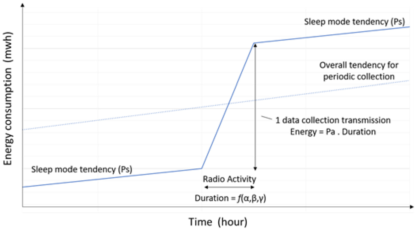
Radio interface consumption model for a node (one collection cycle).

If all nodes have the same material characteristics, tendencies (slopes induced by Ps and Pa) will be the same for all nodes involved in a chain. Only duration activity will change and so impact the energy consumed by the nodes. Our models allow quantifying the potential energy gain involved by using (or not using) aggregation for chain data collection. Because these parameters do not evolve in time and if, during application, the required collection frequency does not change too, the total energy spent by a node can be directly obtained with the number of collection cycle. In this approach, the consumed energy at node depends on device characteristics (Pa and Ps), on the communication structure (chain) and on the collection and network communication protocols (activity duration).

These simple and effective models can be used online by nodes for remaining energy self-assessment. Distributed routing algorithms can use the consumed energy to determine or maintain the communication structure. Models can also be used by an external software control system to have a global and centralized vision of the spent energy of all nodes of the network.

Conclusion and future works

In this article, the McBIM project has been presented as well as the concept of communicating concrete and the challenges faced by it from manufacturing to exploitation. Energy saving and consumption assessment of nodes within a communicating concrete element is the focus of this article. Energy consumption models, representative chain-based routing protocols, and time synchronization mechanisms for WSN are discussed for positioning this work. Analytic energy consumption models of a chain-based WSN with or without aggregation are proposed. A chain-based data collection approach is presented where both sleep mode and data aggregation process are considered. The models were verified by a chain experiment platform. Data collection tests realized both on the three-node and six-node chain structures prove that our strategy is efficient for periodic data collection. Using sleep mode combined with data aggregation greatly reduces energy consumption. According to the node’s position in the chain, the reduction can be quantified by the gap of activity duration between the two collection modes (with or without aggregation). Another result is that the proposed estimation models for energy consumption can be validated because they match the real experiments.

In following works, we will improve, test, and adapt energy estimation models to other aggregation routing protocols and communication structure (tree-based and cluster-based). Extended experimentations could be made in order to consolidate models. Three kinds of campaigns can be envisaged: (1) Long-time experimentations to verify that the models do not drift from reality with time; (2) Experimentations with a longer chain structure to experimentally confirm the gap between collection with or without aggregation; (3) Experimentations with other wireless technologies to compare performances.

We do not yet know the density of nodes necessary for our application in concrete. But we can now estimate the lifetime of the communicating concrete according to collection frequency. This work allows to determine the operating limits of the services of a McBIM element according to the density of the nodes inserted in the concrete. Moreover, with these measured physical parameters, a three-dimensional estimation model could be built with simulation software for further study. The behaviors of communicating concretes in energy cost from manufacturing to exploitation can then be estimated and analyzed. It gives a fast and accurate lifetime estimation for the real wireless CNs inserted in material.