Sage Journals: Discover world-class research

Abstract

The device-free localization that locates an uncooperative target by analyzing its shadowing effect on wireless links in low-cost wireless sensor networks has become an attractive technique. Due to its ability of realizing localization without the need of equipping the target with any wireless device, device-free localization has lots of potential applications ranging from emergency rescue to patient monitoring. However, since the change of the received signal strength on links easily becomes unpredictable due to all kinds of dynamical factors, device-free localization is still a challenging problem. In this article, we propose a novel two-step sequential device-free localization method to enhance device-free localization performance. The sequential device-free localization first utilizes the geometric-based method to quickly obtain the coarse positioning result with low storage and computational requirements, and then exploits the location information of selected wireless nodes to improve the accuracy of the geometric-based localization result based on the optimization-based method, which ensures its robust performance. Experimental results in indoor and outdoor scenarios demonstrate the effectiveness and robustness of the proposed scheme.

Keywords

Device-free localization quasi-distance localization approach received signal strength two-step sequential method wireless sensor networks

Introduction

Target localization and tracking techniques in wireless sensor networks have received lots of attentions during the past two decades since the position information is extremely valuable for commercial and military applications. Generally, the localization research can be divided into cooperative and non-cooperative localization. Unlike cooperative localization techniques that equip the target with a wireless device such as a radio frequency identification (RFID) tag, device-free localization (DFL) is a new concept that allows the localization and tracking for targets which neither carry any devices nor participate actively in the localization process.^1,2 DFL technologies are particularly useful in a wide number of applications including intrusion detection, border protection, emergency rescue, patient or elder monitoring, and so on, where targets being tracked cannot be expected to cooperate with the localization system.

Conventional DFL methods utilize ultra-wideband (UWB) radar, video cameras, or infrared sensors to passively localize targets. These methods are limited by the deployment cost, privacy concerns, or their poor capability of penetration. Different from these techniques, the low-cost DFL which relies on received signal strength (RSS) measurements has recently become a promising technique and shown lots of potential applications. Nowadays, most wireless transceivers can easily measure the RSS during the normal communicating process, so it is convenient to use RSS measurements as coarse sensors for DFL.¹ Moreover, compared with conventional DFL methods, the RSS-based DFL approach has some merits on practical applications. It can not only work in obstructed scenarios with its ability of seeing through smoke, darkness, and walls but also avoid the privacy concerns raised by video cameras.

The basic principle of RSS-based DFL is that when a target moves into the area within a wireless network, it may cause the changes of RSS by shadowing, reflecting, diffracting, or scattering. The shadowed links will be different when a target locates at different locations, and this makes it possible to realize DFL based on the link measurements.^3–9 However, due to the dynamic and sensitive nature of RSS, a slight variation of the environment will cause the changes of RSS measurements. Moreover, there are lots of other factors besides the presence of the target that can affect the variations of RSS, and therefore, the change in RSS due to target presence becomes unpredictable. To enhance the DFL performance, a number of RSS-based DFL algorithms have been proposed in recent years including the model-based method, the training-based method, the geometric-based DFL (GDFL) method, and so on. While the aforementioned methods have their respective merits, RSS-based DFL is still a challenging problem due to the uncertain and dynamic RSS character in indoor and outdoor environments. In this article, we propose a novel two-step sequential method to solve the DFL problem, which first utilizes the geometric-based method to quickly obtain the coarse positioning result and then exploits the location information of wireless nodes to improve the accuracy of the localization result based on the optimization-based method. The main contributions of this article are summarized as follows:

A robust two-step sequential DFL method (SDFL) is proposed. The algorithm uses simple geometric operations to generate the coarse estimation of the target’s position, which can keep the merits of low storage and computational requirements. On the basis of the coarse location, the low-complexity optimization-based method is used to enhance the accuracy of the localization result. Hence, this algorithm combines advantages of two different methods into a unified DFL process.

In the published DFL methods, wireless nodes mainly take charge of communicating and measuring RSS values. In fact, the location information of wireless nodes is not only known a priori but usually accurate as well, so we can use this useful information as an assisted condition to enhance the DFL accuracy. Unlike the previous DFL methods that node location information is only implicitly exploited to form line segments or represent the focus of an ellipse, the SDFL method explicitly utilizes the knowledge of nodes’ coordinates to improve the DFL accuracy.

A quasi-distance localization approach based on the optimal selected nodes is proposed to merge node location information into the SDFL method. The quasi-distance-based algorithm in the second step still does not assume any prior knowledge of the shadowing model or need any offline training, so it keep the merits of the geometric-based method in the first step.

The remainder of the article is organized as follows. “Related works” section presents the related works. The problem formulation is described in “Problem formulation” section. The details of the two-step SDFL algorithm are addressed in “Two-step sequential DFL algorithm” section. “Experimental results” section gives the experimental setup and experimental results. Finally, “Conclusion” section concludes the article.

Related works

In past decades, lots of research works have been carried out to realize the cooperative localization or tracking technique that requires the target to equip with a wireless device like a smartphone or a RFID tag and to cooperate with the special localization system. Various approaches have been proposed and tested in different scenarios of practical interest.^10–12 Besides numerous works dedicated to applications in cooperative localization or tracking, there already exist some surveys^13–15 that provide a comprehensive analysis about the cooperative positioning technology. The interesting readers can refer to these literature.

In this section, we primarily summarize the most relevant research on the DFL. As a promising technique, many RSS-based DFL approaches have been developed, and most of them can be classified into three categories. One main approach of DFL is to model the RSS variation, due to the shadowing or reflection of the target, as a function of the target’s position. In Wilson and Patwari,³ an elliptical model is introduced to describe the spatial impact area when a target appears on a wireless link. This elliptical model assumes that the RSS of the link will change when a target locates inside the ellipse. Otherwise, the RSS will remain unchanged. Based on this elliptical model and motivated by computed tomography, Wilson and Patwari formulates a method termed as radio tomographic imaging (RTI) that estimates the RSS changes in the radio frequency (RF) propagation field of the interested area and then forms an image of the target-affected field by using a regularization method. This image is then used to infer the targets’ location within the deployed network. The localization performance of RTI may be further enhanced with the assisted techniques, such as frequency diversity,⁴ antenna diversity,⁵ power diversity,⁶ and compressive sensing.^7,8 Furthermore, some recent work explores the use of radio tomography in highly obstructed areas for the purpose of tracking moving objects through walls.^16,17 To improve the elliptical model, Hamilton et al.¹⁸ proposed a novel inverse area elliptical model (IAEM), which defines that the shadowing effect of a target on a wireless link is inversely proportional to the size of the smallest ellipse that contains the target. Based on the diffraction theory or extensive experimental data, the exponential-Rayleigh model (ERM),¹⁹ the diffraction model (DM),²⁰ and the saddle surface model (SaS)²¹ are recently proposed to model the RSS changes, and they are all incorporated into the particle filter framework to realize DFL. Although these novel models significantly enrich the research of the model-based DFL, lots of experiments have demonstrated that RSS is time-varying at different locations within the spatial impact area, and RSS even may change without human motion in the deployment area. Since most previous models that are obtained empirically or constructed according to the diffraction theory only describe the shadowing effect under the ideal conditions, they generally cannot be accurate enough to model RSS variations in real dynamical environments. Therefore, model errors are unavoidable when these models are directly used to realize RTI.

Another RSS-based DFL method is the training-based method, which matches the RSS samples collected online with the offline-constructed radio map. The procedure is similar to the fingerprinting in cooperative localization.²² This method for DFL is originally proposed by Youssef et al.,² and then is further developed by Seifeldin et al.²³ and Sabek et al.²⁴ Recently, channel state information (CSI) that can provide a higher dimensional measurement per link is utilized to generalize the radio map for improving DFL performance.²⁵ To enhance DFL performance in the time-varying environment, the training-based method proposed by Mager et al.²⁶ performed lots of experiments to quantify how changes in an environment affect the DFL accuracy. The training-based DFL method can naturally avoid model errors, but the training process is time consuming and labor intensive. Moreover, the radio map needs to be updated once the monitored area changes.

The third category is the GDFL method. Instead of using the shadowing model or the offline training, the GDFL method exploits the link line information affected by targets and simple geometric operations to realize DFL. Zhang et al.²⁷ proposed a particular deployment of wireless nodes and used the overlap of areas formed by shadowed links to estimate the target’s position. However, this method does not exploit spatial prior information about the target’s possible position to filter outlier points, thereby making it sensitive to noise. In order to overcome this shortcoming, Xiao et al.²⁸ proposed a novel nonlinear optimization approach with outlier link rejection for RSS-based DFL. In the geometric-filter (GF) method,²⁹ a threshold value was used to detect the shadowing links, and then a circular prior region was utilized to remove outlier links and points. Finally, the estimate of the target’s position was obtained by the weighted mean of the coordinates of all possible points inside the prior region. Furthermore, an enhanced GF algorithm was proposed by exploiting multichannel RSS measurements to enhance the DFL accuracy in cluttered environments.³⁰ The GF method neither needs to solve the underdetermined problem in model-based DFL nor needs to store the offline fingerprint database, so these characteristics reduce the algorithm’s storage and computational load. However, the weighted mean of all possible intersection points of shadowed links is a coarse approximation. More importantly, the suitable weight values in the GF algorithm are not easily generated, and some empirical weight values sometimes may be unreasonable. Hence, the localization performance of the GF algorithm is not very stable and particularly sensitive to the multipath effects.

Problem formulation

A DFL system is composed of M wireless nodes with known locations deployed around the area of interest, such as that shown in Figure 1. Each wireless node can transmit or receive radio signals at each time instant, and thus there are L = M(M – 1)/2 bidirectional links traveling through the monitored region. As shown in Figure 1, the links traveling through a target are shadowed due to scattering, reflection, diffraction, or absorption. Obviously, the target-affected links due to the target’s presence will be different when a target locates at different locations. Hence, it is possible to realize DFL based on the link information involved in the RSS measurements.^1,2

Figure 1.

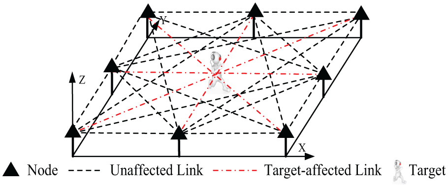
A DFL system made up of eight nodes.

In this article, all wireless nodes are coplanar with the single target to be tracked and are assumed within radio range of each other. Let the line segment l_i represent the link i from the node $n_{i}^{a}$ at location coordinate $(x_{i}^{a}, y_{i}^{a})$ to the node $n_{i}^{b}$ at location coordinate $(x_{i}^{b}, y_{i}^{b})$ , and then the set of all links can be defined as $Z = {l_{i}, i = 1, 2, \dots, L}$ .

Generally, the RSS of link i measured at time t can be represented as³

y_{i} (t) = P_{i} - J_{i} - S_{i} (t) - F_{i} (t) - v_{i} (t)

(1)

where P_i represents the transmitted power, S_i(t) represents the shadowing loss of link i due to the attenuation caused by the target, F_i(t) represents the fading loss, and J_i is the static losses because of antenna patterns or device inconsistencies. v_i(t) represents other losses affected by noise. Thus, the RSS variation at time t can be represented as

Δ y_{i} (t) = y_{i} (t) - y_{i} (0) \approx - S_{i} (t) + n_{i} (t)

(2)

where $n_{i} (t) = F_{i} (0) - F_{i} (t) + v_{i} (0) - v_{i} (t)$ and y_i(0) represents the baseline RSS measurement that is obtained when the monitored area is vacant. The baseline information can also be estimated online by using the approach proposed by Zhao and Patwari.³¹ Since Wilson and Patwari³ has demonstrated that noise n_i(t) is generally insignificant compared with the shadowing loss, the RSS variation △y_i(t) is mainly determined by the shadowing loss. For clarity, let $y_{t} = [y_{1} (t) y_{2} (t) \dots y_{L} (t)]$ represent RSS measurements for all L links when the target appears at time t, and let $y_{0} = [y_{1} (0) y_{2} (0) \dots y_{L} (0)]$ be baseline RSS measurements for all L links when the deployment area is vacant. Correspondingly, the vector of RSS variations for all links is given as $Δ y_{t} = [Δ y_{1} (t) Δ y_{2} (t) \dots Δ y_{L} (t)]$ , that is, Δy_t = abs[y_t – y₀], where abs[ ] is the operation of absolute value.

The aim of a DFL system is to acquire the high-precision target coordinates at time t, with the information of RSS measurements y₀ and y_t and the accurate positions of the M wireless nodes.

Two-step sequential DFL algorithm

This section introduces the proposed SDFL algorithm in detail. As shown in Figure 2, the SDFL algorithm includes the GDFL part and the optimization-based DFL part. While the geometric-based part of the SDFL algorithm shares some features with the previous GDFL algorithm,^29,30,32 the concrete approach is definitely different. Moreover, the subsequent optimization-based DFL part based on the location information of wireless nodes is not included in these methods.

Figure 2.

Algorithm framework for localizing a target.

GDFL method

The basic idea of the GDFL method is that the shadowed links affected by a target tend to intersect with each other at points near the target’s true position, and therefore, the key step of GDFL is to find the target-affected links. Due to the presence of noise and multipath effects, RSS variations are not stable and even RSS may vary without human motion in the monitored area. Therefore, even if some links do not go through the target’s vicinity, the RSS measurements of these links may obviously vary. Hence, it is necessary for the geometric-based method to remove outlier links before estimating the target’s position. Based on the above analysis, the geometric-based part of the SDFL algorithm includes the following steps: effective links identification, removing outlier links via spatial prior information, and generating a position estimate. Unlike the earlier work,^29,30,32 we adopt the non-weighted mean method to estimate the target’s position for avoiding the difficulty of acquiring the reasonable weights. Moreover, the spatial prior region is modified in “Removing outlier links via spatial prior information” subsection.

Effective links identification

Some previous DFL experiments have demonstrated that the RSS on a wireless link may be distinctly attenuated or amplified since the appearance of the target will cause some links to be shadowed.^4,6 Therefore, if the link i is shadowed by a target, the corresponding RSS change of the ith link must be above the shadowing detection threshold. To pick out the target-affected links, let y_th represent the shadowing detection threshold which can be obtained experimentally. Thus, the set Z_t is defined as the target-affected link set when Z_t contains all effective links that RSS variations are larger than the detection threshold at time t, that is

Z_{t} = {l_{i} | Δ y_{i} (t) > y_{th}}

(3)

Since the RSS fluctuation affected by noise is usually less than the detection threshold y_th, the noise influence is alleviated by using the simple threshold detection method, and only the significant links that the RSS measurements evidently vary are selected.

Removing outlier links via spatial prior information

Although the last step of GDFL alleviates the negative effect of noise, the RSS variations in some wireless links that are not near the target may be also above the threshold value y_th because of multipath effects.^27,28 As shown in the work of Talampas and Low,^29,30 outlier links may intersect with other effective links at points far away from the target, so outlier links that are not excluded from the localization process will result in large tracking errors. To remove the negative effect of such outlier links on the target position estimate, there are two kinds of approach to distinguish the target-affected links and the outlier links. One approach exploits the spatial prior information to choose the target-affected links,^29,33,34 while another approach identifies the outlier links based on the standard variance of the measurement noise.³⁵ In this article, we also make use of the same idea in the work of Talampas and Low²⁹ and Wang et al.^33,34 that spatial prior information is used to pick out the real target-affected links from the set Z_t. However, in a DFL system, we can obtain little knowledge about the target due to the non-cooperative characteristic of DFL. Here, we only can exploit the information about the target’s previous location estimate and the assumption about probable maximum speed of the target to construct the spatial prior region. When the target’s location p_t−11 = (x_t, y_t₋₁) at time t – 1 is regarded as the center of the circular spatial region, the prior region R_t at time t can be described as the following circle, that is

R_{t} = {p_{t} | E (p_{t - 1}, p_{t}) < r}

(4)

where p_t represents the position vector of a possible point inside the monitored area, and E(p_t−1, p_t) defines the Euclidean distance between the positions p_t−1 and p_t. The radius r of the circular prior region depends on the distance that the target can move in the sampling interval △t, that is, r ≥ u_max × △t, where u_max is the target’s maximum speed. From Figure 3, we can find that the possible candidate positions of the target at time t must locate in the predicted prior region R_t. Hence, those links in Z_t that do not intersect the circular region R_t can be regarded as the outlier links. Based on the simple geometric calculation, it is easy to pick out the outlier links from Z_t. For the link i, the straight line equation can be represented as y = k_ix + b_i, where the slope k_i is $(y_{i}^{b} - y_{i}^{a}) / (x_{i}^{b} - x_{i}^{a})$ and the intercept b_i is $y_{i}^{a} - {kx}_{i}^{a}$ . Then, according to the geometric knowledge, the shortest distance between the circular center p_t−1 and the link i can be calculated as

d_{i} (t) = \frac{| k_{i} x_{t - 1} - y_{t - 1} + b_{i} |}{\sqrt{1 + k_{i}^{2}}}

(5)

Since the shortest distance between the outlier link and the circular center p_t−1 must be greater than the radius r, the set of effective links that excludes the outlier links can be represented as

{\bar{Z}}_{t} = {l_{i} | d_{i} (t) < r and l_{i} \in Z_{t}}

(6)

However, as shown in Figure 3, if the target locates at the boundary of the prior region R_t, some links outside the prior region but near the real-line circle may also be affected by the target. Therefore, the radius of the prior region should be extended to (1 + m)r, and the set of effective links that intersect the extended prior region should be modified as

{\tilde{Z}}_{t} = {l_{i} | d_{i} (t) < (1 + m) r and l_{i} \in Z_{t}, m \in (0, 1)}

(7)

where m is a positive decimal fraction between 0 and 1. The equation (7) means that when d_i(t) > (1 + m)r, the link i can be considered as a outlier link.

Figure 3.

Illustration of effective links and the circular prior region.

Using triangle centroids to generate a position estimate

After identifying the effective links and removing the outlier links, assume that there are J (J ≤ L) links remaining in ${\tilde{Z}}_{t}$ that can be considered as the real effective links affected by the target. In the previous work of Talampas and Low,²⁹ the intersection points of the effective links in ${\tilde{Z}}_{t}$ represent the potential positions of the target, and then the target’s position estimate is acquired by using the weighted mean method. However, the proper weight is difficult to be obtained. There are no reasonable physical explanations for the RSS-based weight and the distance-based weight that are used in the previous work of Talampas and Low.²⁹ For example, the distance-based weight depends on the distance between the intersection point and the circular center p_t−1. Under this kind of weight, those points that are closer to the circular center p_t−1 are assigned higher weights as compared to farther points. However, in fact, it is unknown whether the true target’s position is close to the circular center p_t−1 and the target may locate at the border of the prior region.

To avoid the difficulty of generating proper weights, in this article, we seek an approximate result by using the non-weighted mean method. The experimental results in “Experimental results” section will demonstrate that the non-weighted GDFL method can provide the almost same localization performance as the weighted mean method. Meanwhile, different from solving for the link intersections in the work of Talampas and Low,²⁹ we use centroid points of virtual triangles consisting of effective links to represent the target’s potential positions. This is based on the consideration that a target will affect its ambient links rather than only two links. Since there are a total of J effective links in ${\tilde{Z}}_{t}$ and any three links can form a virtual triangle, there will be maximum W ( $W \leq C_{J}^{3}$ ) triangles, and each triangle generates a centroid position. Different from the weighted mean method in the work of Talampas and Low²⁹ and Li et al.,³² the estimate of the target’s coordinate (x_s, y_s) is calculated by directly averaging all the centroids’ coordinates, that is

x_{s} = \frac{1}{W} \sum_{j = 1}^{W} x_{j}, y_{s} = \frac{1}{W} \sum_{j = 1}^{W} y_{j}

(8)

where (x_j, y_j) is the centroid coordinate of the jth virtual triangle. Figure 4 depicts an example of how to acquire the estimated position of the target by averaging the centroids’ coordinates of three triangles.

As shown in Figure 4, it can be observed that not all centroids of triangles lie inside the circular prior region. The position of each centroid represents a potential position of the target, so those centroids that locate outside the prior region should be regarded as the outlier target points. Similarly, the circular prior region can be used again to remove these outlier points. In other words, when $E (p_{t - 1}, c_{t}^{j}) > r$ , the jth centroid can be identified as an outlier point, where $c_{t}^{j}$ represents the position vector of the jth centroid at time t. Assuming that there are $\tilde{W}$ ( $\tilde{W} \leq W$ ) centroid points inside the circular prior region, the target’s coordinate will be adjusted as

x_{s} = \frac{1}{\tilde{W}} \sum_{j = 1}^{\tilde{W}} x_{j}, y_{s} = \frac{1}{\tilde{W}} \sum_{j = 1}^{\tilde{W}} y_{j}

(9)

Figure 4.

Illustration of the non-weighted triangle localization method.

Optimization-based DFL method

Improving the geometric localization result by using node location information

Although the above GDFL method only needs using elementary geometric operations to realize DFL, the estimated result from the GDFL method is only a coarse approximation due to simply using the mean of the triangle centroids as the target location. In addition, the GDFL is particularly sensitive to multipath effects. Therefore, the geometric localization result $r_{s} = (x_{s}, y_{s})$ usually deviates from the true target position $r_{0} = (x_{0}, y_{0})$ .

In order to improve the geometric-based localization result, the basic idea of the optimization-based DFL method is to merge node position information into the DFL process based on the fact that generally the position information of wireless nodes is accurately known before they begin to work. Under the constrained least squares (LS) framework,³⁶ in this article, a quasi-distance-based DFL method is proposed by exploiting node position information to enhance the DFL accuracy. It should be noted that in this step, the target still does not carry any device. Hence, different from the device-based localization that can directly measure distances between the target and nodes by using the device-to-device method, we use the estimated distances between the coarse position of the target and wireless nodes to substitute the measuring distances in the device-based localization. We refer to this kind of distance as quasi-distance. Thus, this method can continue to maintain the merit of DFL that need not carry any device, and at the same time the accurate position information of nodes is utilized to improve the geometric-based localization result. In addition, in order to determine which node is better to participate in the optimization, we exploit the geometry effects of node configurations to select most suitable nodes in each optimization.

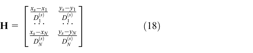
Based on the position coordinate $r_{s} = (x_{s}, y_{s})$ , the estimated distance between the coarse position of the target and the nth wireless node is

D_{n}^{(s)} = ‖ r_{n} - r_{s} ‖ = \sqrt{{(x_{n} - x_{s})}^{2} + {(y_{n} - y_{s})}^{2}}

(10)

where $r_{n} = (x_{n}, y_{n})$ is the coordinate vector of the nth node and ‖•‖ represents the Euclidean norm. However, the true distance between the target and the nth node is

D_{n}^{(0)} = ‖ r_{n} - r_{0} ‖ = \sqrt{{(x_{n} - x_{0})}^{2} + {(y_{n} - y_{0})}^{2}}

(11)

Thus, the error between the estimated and accurate distances can be represented as

\begin{matrix} e_{n} = \frac{1}{2} ({‖ r_{n} - r_{0} ‖}^{2} - {‖ r_{n} - r_{s} ‖}^{2}) = - r_{n}^{T} r_{0} + r_{n}^{T} r_{s} \\ + \frac{{‖ r_{0} ‖}^{2}}{2} - \frac{{‖ r_{s} ‖}^{2}}{2} \end{matrix}

(12)

where $‖ r_{0} ‖ = \sqrt{x_{0}^{2} + y_{0}^{2}}$ and $‖ r_{s} ‖ = \sqrt{x_{s}^{2} + y_{s}^{2}}$ . If there are N (N ≤ M) nodes participating in the optimization-based DFL, we can put all N errors together and write them in the following vector form

e = A θ - b

(13)

where $e = [e_{1} e_{2} \dots e_{N}]^{T}$ , $θ = [x_{0} y_{0} R_{0}]^{T}$ , $A = [\begin{matrix} - x_{1} & - y_{1} & 1 / 2 \\ \dots & \dots & \dots \\ - x_{N} & - y_{N} & 1 / 2 \end{matrix}]$ , $b = [\begin{matrix} R_{s} / 2 - x_{1} x_{s} - y_{1} y_{s} \\ \dots \\ R_{s} / 2 - x_{N} x_{s} - y_{N} y_{s} \end{matrix}]$ , $R_{0} = ‖ r_{0} ‖^{2}$ , and $R_{s} = ‖ r_{s} ‖^{2}$ . The corresponding LS criterion is then given by

min_{θ} {(A θ - b)}^{T} (A θ - b)

(14)

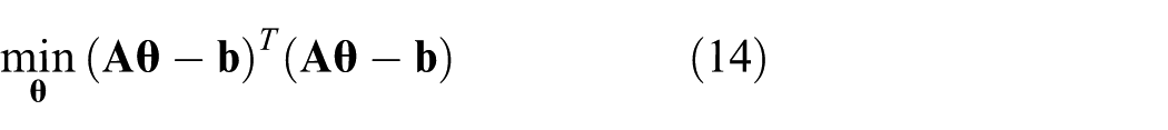
subject to a quadratic constraint

q^{T} θ + θ^{T} P θ = 0

(15)

where P = diag(1,1,0) is a diagonal matrix, and q = [0 0 –1]^T. The constrained LS solution using the technique of Lagrange multipliers is given by (see Appendix 1)

θ = {(A^{T} A + λ P)}^{- 1} (\frac{A^{T} b - λ q}{2})

(16)

where λ is determined in Appendix 1.

Node selection

The remaining problem of the optimization-based DFL is how to determine which node is better to participate in the optimization. In fact, the scheme that all M nodes join in the optimization process is not a good method, because it will result in high computational load due to the high dimensions of matrix A and vector b. More importantly, when all nodes are used, the geometric effect of node configuration is not always best on localization accuracy according to the geometric dilution of precision (GDOP) concept. In fact, since there are only two parameters to estimate, theoretically three non-collinear nodes are enough. For good positional accuracy of the optimization-based DFL, we make use of the best (lowest) GDOP to select N nodes with best geometric configuration in each experiment.

Based on the GDOP analysis in the work of Levanon³⁷ and Sharp et al.,³⁸ the GDOP will be given by

GDOP = \sqrt{G_{11} + G_{22}}

(17)

where G₁₁ and G₂₂ are the diagonal elements of the matrix $G = (H^{T} QH)^{- 1} / σ^{2}$ , and σ is the root mean square (RMS) value of each measurement. H is the Jacobian matrix of partial derivatives of the measurement equations with respect to the unknown parameters, which can be computed as

H = [\begin{matrix} \frac{x_{s} - x_{1}}{D_{1}^{(s)}} & \frac{y_{s} - y_{1}}{D_{1}^{(s)}} \\ \dots & \dots \\ \frac{x_{s} - x_{N}}{D_{N}^{(s)}} & \frac{y_{s} - y_{N}}{D_{N}^{(s)}} \end{matrix}]

(18)

Q is the error covariance matrix. Since the transceivers of the nodes are generally the same devices, the errors in all measurements can be considered having the identical RMS value σ. Thus, Q = σ² I , where I is an N × N identity matrix. Then, the matrix G can be simplified as

G = {(H^{T} H)}^{- 1}

(19)

Once the matrix G is determined, the GDOP value is easily obtained by equation (17). When a DFL system is composed of M nodes which evenly distribute on the perimeter of a square area, there are $C_{M}^{N}$ node selection methods in the above optimization-based DFL. However, those combinations that N nodes are on the same straight line must be excluded, so the total of possible node selection methods is $C_{M}^{N} - C_{M / 4 + 1}^{N} \times 4$ . By comparing with these GDOP values, we can find a best node configuration for the optimization-based DFL when the corresponding GDOP is lowest.

However, it should be emphasized that the GDOP value should be computed for every new position, while it can reduce the size of matrix A and vector b. For GDOP, the computation mainly involves the operations of matrix inverse and multiplication. The complexity of the matrix inverse operation is O(N³), and the multiplication operation is O(N²), where N represents the dimension of the matrix. In order to overcome this shortcoming of the optimization-based method and keep the low-complexity merit of GDFL, we divide the monitoring area into G grids, where each grid represents one possible target’s position if making the grid enough dense. Therefore, we can compute all the GDOP values for each grid beforehand, and correspondingly obtain the best node combination for each possible target’s position. Although too dense grid may result in large computation time in the offline stage, in the online stage, we can directly obtain the best node selection to participate in the optimization by simply matching the geometric-based localization coordinates with the grids’ coordinates.

Experimental results

Experimental setup

To demonstrate the applicability of the SDFL method, we develop a prototype DFL system which is made up of 24 wireless nodes in an open outdoor environment (Scene 1) or 16 wireless nodes in a rich multipath indoor scenario (Scene 2) to carry out extensive experiments. The photographs and layout of the deployment area are shown in Figure 5, where a target (a person) moves clockwise along a predefined trajectory and its location is estimated once per second. A metronome and uniformly placed markings on the floor help the experimenter to take constant-sized steps at a regular time interval, and the target’ moving speed is about 1.0 m/s. In the outdoor experimental environment, wireless nodes are placed 1.5 m apart along the perimeter of a 9 × 9 m square area being free from obstructions, while 16 nodes are deployed to cover a 8 × 8 m laboratory area where there are numerous obstructions such as tables and other equipment. Although it is not necessary to place the nodes in a uniform spacing, in this article, all wireless nodes are evenly spaced at the perimeter of the deployment region for simplicity. In all experiments presented in the following sections, the baseline RSS measurements are first taken for calibration. The calibration stage lasts for approximately 60 s when the target is not inside the monitored area.

Figure 5.

Experimental networks: (a) photograph of the uncluttered outdoor environment, (b) geometry of the uncluttered outdoor environment, (c) photograph of the highly cluttered indoor environment, and (d) geometry of the highly cluttered indoor environment.

The transceiver of each node is a TI CC2530 device operating on the 2.4 GHz ISM band with IEEE 802.15.4 standard, which is placed on a tripod that is 1 m above the ground. To ensure regular network transmission, a token ring protocol is adopted to guarantee the stability of the networks and control transmissions. Every node has its ID number and broadcasts its link information in turn with the transmission interval 5 ms in our experiments. During the transmitting period of each node, all other nodes receive data packets and measure the RSS of the link from the transmitter to themselves. The information packets of each transmitting node includes the ID of the node and the most recent RSS measurements of the links between all other nodes and itself. A data-acquisition node listens to all network broadcasts from the measurement nodes and transfers the RSS data to a laptop computer with 3.5 GHz processor and 8 GB memory via a UART port.

Performance evaluation and comparison

Here, we compare the performance of the two-step SDFL method with two types of algorithms, that is, the geometric-based GF algorithm²⁹ and the model-based RTI algorithm³ in both outdoor and indoor scenarios. For the sake of fairness, the one-step GDFL algorithm without using the node location information is also used in the following experiments for comparisons. The default parameters are summarized as follows: the radius of the prior region is set as 1.5 m, and the detection threshold is 4 dB in GF, GDFL, and SDFL. In the SDFL method, four nodes are selected to participate in the optimization according to the analysis in Figure 7(c) and m is 0.2. The parameters used in the RTI algorithms are summarized as follows: the width of the ellipse is 0.15 m, regularization parameter is 4.5, and the number of grids is 3600. For high reliability, all the localization results are obtained from the average of 50 independent experiments.

Figure 6(a) and (b) show the tracking errors of the SDFL, GDFL, GF, and RTI methods, respectively. In Figure 6, it can be observed that the two-step SDFL algorithm has the least tracking error in both indoor and outdoor scenarios. Especially, the SDFL algorithm is superior to the one-step GDFL method, which proves the effectiveness of the proposed optimization-based method by exploiting the position information of nodes. Meanwhile, it should be noted that the tracking error is periodically relatively large for some seconds. This can be attributed to the fact that when the target locates at the corners, there will be fewer target-affected links.

Figure 6.

The comparisons of tracking errors: (a) Scene 1 and (b) Scene 2.

The detailed statistical data about tracking errors are summarized in Tables 1 and 2. In Table 1, we can see that the tracking performance of the SDFL algorithm is better compared with the GDFL, GF, and RTI methods in the uncluttered outdoor environment, with the mean tracking error reduced by 0.171, 0.191, and 0.378 m, respectively. Meanwhile, we can see that although the GDFL uses the non-weighted method to calculate the position of the target, the tracking performance of the GDFL method is similar with that of the GF algorithm.

Table 1.

Comparisons of tracking errors—Scene 1.

Algorithm	Mean (m)	Median (m)	RMSE (m)
SDFL	0.398	0.450	0.501
GDFL	0.569	0.660	0.696
GF	0.589	0.635	0.712
RTI	0.776	0.776	1.039

RMSE: root mean square error; SDFL; sequential device-free localization; GDFL: geometric-based device-free localization; GF: geometric-filter; RTI: radio tomographic imaging.

Table 2.

Comparisons of tracking errors—Scene 2.

Algorithm	Mean (m)	Median (m)	RMSE (m)
SDFL	0.681	0.711	0.703
GDFL	1.013	0.951	0.993
GF	1.009	0.976	0.976
RTI	1.285	1.093	1.581

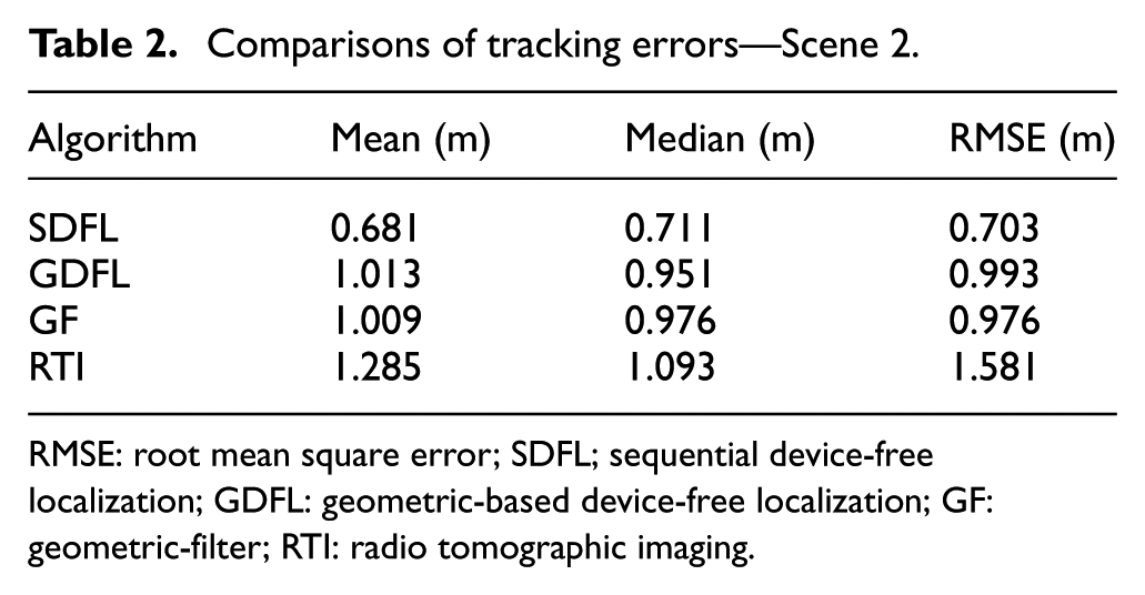
RMSE: root mean square error; SDFL; sequential device-free localization; GDFL: geometric-based device-free localization; GF: geometric-filter; RTI: radio tomographic imaging.

Different from the outdoor environment, multipath effects cause higher RSS fluctuations in the cluttered indoor scenario, and thus, the tracking errors of all algorithms become larger in the indoor environment by comparison between Tables 1 and 2. However, the two-step SDFL method can still achieve the highest tracking accuracy, and the mean tracking error of SDFL is still less than 1 m. In addition, the RMSE of the two-step SDFL algorithm is improved by 29.2%, 28.0%, and 55.5% when compared with the GDFL, GF, and RTI methods, respectively. These results show that the two-step SDFL approach can provide the stablest localization performance among all the methods in the highly cluttered indoor environment.

Discussion

In this subsection, to further evaluate the robustness of the two-step SDFL algorithm, we examine the impact of different parameters including radius of the circular prior region, detection threshold, and the number of nodes that take part in the optimization-based process. Figure 7(a) shows the effects of the different radius r on the tracking performance for both scenes. From Figure 7(a), we can clearly find that the tracking error is large when the radius r is big, because too many outlier links are allowed to be involved in the GDFL process under this condition. On the contrary, since the target may travel outside the prior region when the radius r is too small, the tracking error will also increase due to the misuse of spatial prior information. These phenomena are consistent with the description of equation (7), which has shown that the radius of the prior region determines how many outlier links are removed. In Figure 7(a), the tracking performance of SDFL is good when the radius r is between 1.2 and 1.7 m for Scene 1 and between 1 and 1.6 m for Scene 2. The tracking errors will increase when the value of radius is outside the above scopes.

Figure 7.

Performance comparisons under different parameters: (a) tracking performance under different radius of the circular prior region, (b) effects of different detection threshold values, and (c) effects of the different number of nodes that take part in the optimization-based process.

Then, the performance of the SDFL algorithm is evaluated under different threshold values. From Figure 7(b), the tracking performance of SDFL is good when the threshold value is between 3 and 7 dB for Scene 1 and between 3 and 5 dB for Scene 2. This attributes to the fact that the higher detection threshold will result in fewer detected effective links and then generate less centroids that can be regarded as the target’s possible positions. On the contrary, if the threshold value is set too low, the geometric-based algorithm will become more susceptible to noise, especially in the rich multipath indoor scenario. In addition, from Figure 7(b), we can find that the range of good threshold values in Scene 1 is larger than that in Scene 2. For Scene 1 with M = 24 nodes and the monitored area S = 81 m², the average link density ρ is 3.41/m², while the average link density ρ = 1.88/m² in Scene 2 with M = 16 nodes and the monitored area S = 64 m². Therefore, with the same radius r = 1.5 m in both scenes, the average number of links crossing prior region N_L = πr²ρ are 24.07 for Scene 1 and 13.25 for Scene 2, respectively. Due to the higher average link density, even if the high threshold value is set in Scene 1, there are similar number of effective links as the low threshold value in Scene 2.

The tracking errors under different numbers of nodes that take part in the optimization process of SDFL are illustrated in Figure 7(c). We can find from Figure 7(c) that it is not conspicuous for the improvement of the tracking accuracy when more nodes participate in the optimization process. Moreover, the tracking accuracy decreases slightly when the number of nodes increases to seven or higher. Generally, the position information of four to six nodes are enough to enhance the localization precision, which can help to have a good trade-off between the tracking performance and computational complexity.

At last, Figure 8 gives the average running time required to generate one position estimate for four algorithms in both indoor and outdoor scenes. Although the RTI method has the need of solving the matrix inverse problem, the matrix inverse operation of RTI needs only to be calculated once. Therefore, the matrix inverse time of RTI is not included in the total running time of RTI. Thus, what the RTI technique needs to perform in each execution is the multiplication of a known matrix and a measurement vector. Therefore, its running time can be very low in Figure 8. Since the geometric-based algorithms’ execution time scales with the number of links in the network, the running time of the GF and GDFL algorithms in Scene 2 is less than that in Scene 1. Due to adding the constrained LS and GDOP step in the SDFL algorithm, the running time of the proposed method is a bit larger than the pure geometric-based method such as the GDFL algorithm. However, since the GDOP values can be calculated in advance, the proposed SDFL algorithm only introduces the small additional computation load. Although the mean execution time for SDFL is higher than the benchmark schemes, the less 0.1 s average execution time for both scenarios can still satisfy the real-time requirement for most DFL applications. Moreover, by optimizing the parameters and reducing the number of nodes, the average execution time of SDFL can be further reduced.

Figure 8.

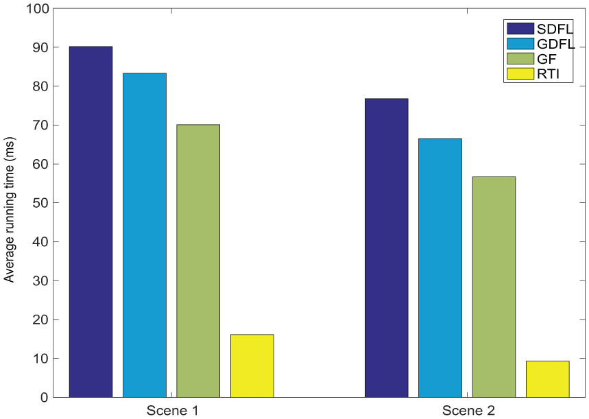
Running times of different algorithms.

Conclusion

To realize high tracking accuracy and suitable computational cost at the same time, a novel two-step SDFL approach is proposed which combines advantages of the geometric-based and the optimization-based DFL methods. In the GDFL part, the shadowed links that are really affected by the target are exploited to create virtual triangles whose centroids are regarded as the potential target positions. In the optimization-based DFL part, the location information of wireless nodes is exploited as an assisted condition to enhance the DFL accuracy. The experimental results in open outdoor and cluttered indoor environments show that the tracking accuracy is improved by using the proposed SDFL method.

It should be mentioned that there are still some problems to be solved. One challenging problem is how to obtain the baseline RSS measurements in the realistic applications. It is difficult to provide vacant deployment area for the baseline RSS measurements such as in the rescue or emergency response operations. Meanwhile, in the proposed scheme, we consider only the scene of tracking one target. How to realize multitarget localization is still an open problem for future research. In addition, the Cramer–Rao lower bound (CRLB) on the position estimation precision needs be considered in the future.

Footnotes

Appendix 1

The minimum of equation (14) under the constraint condition (equation (15)) is obtained by the technique of Lagrange multipliers

(20)

β (θ) = {(A θ - b)}^{T} (A θ - b) + λ (θ^{T} P θ + q^{T} θ)

where λ is the Lagrange multiplier. Necessary conditions for minimizing equation (20) can be obtained by taking the gradient of $β (θ)$ with respect to θ and equating the result to zero, that is

(21)

\frac{\partial β (θ)}{\partial θ} = 2 (A^{T} A + λ P) θ - 2 A^{T} b + λ q = 0

Solving for θ yields the constrained least squares estimate

(22)

θ = {(A^{T} A + λ P)}^{- 1} (\frac{A^{T} b - λ q}{2})

where only λ is yet to be determined. In order to find λ, we can impose the quadratic constraint directly by substituting equation (22) into equation (15), so that

(23)

\begin{matrix} q^{T} {(A^{T} A + λ P)}^{- 1} (\frac{A^{T} b - λ q}{2}) + {(\frac{A^{T} b - λ q}{2})}^{T} \\ {(A^{T} A + λ P)}^{- 1} \times P {(A^{T} A + λ P)}^{- 1} (\frac{A^{T} b - λ q}{2}) = 0 \end{matrix}

By using the eigenvalue factorization, the matrix $(A^{T} A)^{- 1} P$ can be diagonalized as

(24)

{(A^{T} A)}^{- 1} P = U Λ U^{- 1}

where $Λ = diag (γ_{1}, γ_{2}, γ_{3})$ and $γ_{i}, i = 1, 2, 3$ is the eigenvalue of $(A^{T} A)^{- 1} P$ . Substituting equation (22) into $(A^{T} A + λ P)^{- 1}$ gives

(25)

{(A^{T} A + λ P)}^{- 1} = U {(I + λ Λ)}^{- 1} U^{- 1} {(A^{T} A)}^{- 1}

where I is a 3 × 3 identity matrix. Putting equation (25) into equation (23), we get

(26)

\begin{matrix} c^{T} {(I + λ Λ)}^{- 1} a - \frac{λ}{2} c^{T} {(I + λ Λ)}^{- 1} g + e^{T} {(I + λ Λ)}^{- 1} \\ Λ {(I + λ Λ)}^{- 1} a \\ - \frac{λ}{2} e^{T} {(I + λ Λ)}^{- 1} Λ {(I + λ Λ)}^{- 1} g \\ - \frac{λ}{2} c^{T} {(I + λ Λ)}^{- 1} Λ {(I + λ Λ)}^{- 1} a + \frac{λ^{2}}{4} c^{T} {(I + λ Λ)}^{- 1} \\ Λ {(I + λ Λ)}^{- 1} g = 0 \end{matrix}

where c^T = q^TU = [c₁c₂c₃], g = U⁻¹(A^TA)^Tq = [g₁g₂g₃]^T, e^T = b^TAU = [e₁e₂e₃], and a = U⁻¹ (A^TA)⁻¹A^Tb = [a₁a₂a₃]^T. After expanding equation (26), λ is determined from the following equation

(27)

\begin{matrix} \sum_{i = 1}^{3} \frac{c_{i} a_{i}}{1 + λ γ_{i}} - \frac{λ}{2} \sum_{i = 1}^{3} \frac{c_{i} g_{i}}{1 + λ γ_{i}} + \sum_{i = 1}^{3} \frac{e_{i} a_{i} γ_{i}}{{(1 + λ γ_{i})}^{2}} \\ - \frac{λ}{2} \sum_{i = 1}^{3} \frac{e_{i} g_{i} γ_{i}}{{(1 + λ γ_{i})}^{2}} - \frac{λ}{2} \sum_{i = 1}^{3} \frac{c_{i} a_{i} γ_{i}}{{(1 + λ γ_{i})}^{2}} \\ + \frac{λ^{2}}{4} \sum_{i = 1}^{3} \frac{c_{i} g_{i} γ_{i}}{{(1 + λ γ_{i})}^{2}} = 0 \end{matrix}

Therefore, the function of the Lagrange multiplier λ is a polynomial. Due to its complexity, numerical methods have to be used for root searching. After obtaining the Lagrange multiplier λ, the quadratic constraint (equation (15)) is imposed on the final solution.

Handling Editor: Paolo Barsocchi

Declaration of conflicting interests

The author(s) declared no potential conflicts of interest with respect to the research, authorship, and/or publication of this article.

Funding

The author(s) disclosed receipt of the following financial support for the research, authorship, and/or publication of this article: This work was supported in part by the National Natural Science Foundation of China under Grant No. 61405094, in part by the National Key Research and Development Program of China (2017YFB0503500), Jiangsu overseas visiting scholar program for university prominent young and middle-aged teachers and presidents, and Jiangsu Government Scholarship for overseas study.

ORCID iD

Wei Ke

References

Patwari

Wilson

RF sensor networks for device-free localization: measurements, models, and algorithms. Proc IEEE 2010; 98: 1961–1973.

Youssef

Mah

Agrawala

Challenges: device-free passive localization for wireless environments. In: Proceedings of the 13th ACM Mobicom, Montréal, QC, Canada, 9–14 September 2007, pp.222–229. New York: IEEE.

Wilson

Patwari

Radio tomographic imaging with wireless networks. IEEE Trans Mobile Comput 2010; 9: 621–632.

Kaltiokallio

Bocca

Patwari

Enhancing the accuracy of radio tomographic imaging using channel diversity. In: Proceedings of the 9th IEEE international conference on MASS, Las Vegas, NV, 8–11 October 2012, pp.254–262. New York: IEEE.

Bocca

Luong

Patwari

et al . Dial it in: rotating RF sensors to enhance radio tomography, 2013, http://arxiv.org/abs/1312.5480

Wang

Gao

Wang

et al . Device-free localization with multi-dimensional wireless link information. IEEE Trans Veh Technol 2015; 64: 356–366.

Yang

Huang

Guo

et al . A real-time device-free localization system using correlated RSS measurements. EURASIP J Wirel Commu Netw 2013; 1: 1–12.

Wang

Gao

Zhang

et al . Device-free localization with wireless networks based on compressing sensing. IET Commun 2012; 6: 2395–2403.

Kaltiokallio

Jantti

Patwari

ARTI: an adaptive radio tomographic imaging system. IEEE Trans Veh Technol 2017; 66: 7302–7316.

10.

Song

Wang

Shi

et al . Distributed algorithms for energy-efficient even self-deployment in mobile sensor networks. IEEE Trans Mobile Comput 2013; 13: 1035–1047.

11.

Zaidi

Assaf

Affes

et al . Range-free nodes localization in mobile wireless sensor networks. In: Proceedings of the IEEE ICUWB’2015 workshop, Montreal, QC, Canada, 4–7 October 2015, pp.4–7. New York: IEEE.

12.

Zhang

Cao

Chen

et al . Accurate and energy-efficient range-free localization for mobile sensor networks. IEEE Trans Mobile Comput 2010; 9: 897–910.

13.

Liu

Darabi

Banerjee

et al . Survey of wireless indoor positioning techniques and systems. IEEE Trans Systems, Man, and Cybernetics—Part C 2007; 37: 1067–1080.

14.

Gezici

A survey on wireless position estimation. Wireless Pers Commun 2008; 44: 263–282.

15.

A survey of fingerprint-based outdoor localization. IEEE Commun Surv Tutor 2016; 18: 491–506.

16.

Wilson

Patwari

See-through walls: motion tracking using variance-based radio tomography networks. IEEE Trans Mobile Comput 2011; 10: 612–621.

17.

Wang

Xiao

et al . A see-through-wall system for device-free human motion sensing based on battery-free RFID. ACM Trans Embedded Comput Sys 2018; 17: 92–101.

18.

Hamilton

Baxley

et al . Propagation modeling for radio frequency tomography in wireless networks. IEEE J Sel Topics Signal Process 2014; 8: 43–54.

19.

Guo

Huang

Jiang

et al . An exponential-Rayleigh model for RSS-based device-free localization and tracking. IEEE Trans Mob Comput 2015; 14: 484–494.

20.

Wang

Liu

et al . A diffraction measurement model and particle filter tracking method for RSS-based DFL. IEEE J Sel Areas Commun 2015; 33: 2391–2403.

21.

Wang

Gao

Pan

et al . Toward accurate device-free wireless localization with a saddle surface model. IEEE Trans Veh Technol 2016; 65: 6665–6677.

22.

Chan

SHG

. Wi-Fi fingerprint-based indoor positioning: recent advances and comparisons. IEEE Commun Surv Tutor 2016; 18: 466–490.

23.

Seifeldin

Saeed

Kosba

et al . Nuzzer: a large-scale device-free passive localization system for wireless environments. IEEE Trans Mob Comput 2013; 12: 1321–1334.

24.

Sabek

Youssef

Vasilakos

AV.

ACE: an accurate and efficient multi-entity device-Free WLAN localization system. IEEE Trans Mob Comput 2015; 14: 261–273.

25.

Xiao

et al . Pilot: passive device-free indoor localization using channel state information. In: Proceedings of the 33th international conference on distributed computing Systems, Philadelphia, PA, 8–11 July 2013, pp.236–245. New York: IEEE.

26.

Mager

Lundrigan

Patwari

Fingerprint-based device-free localization performance in changing environments. IEEE J Sel Areas Commun 2015; 33: 2429–2438.

27.

Zhang

Chen

et al . An RF-based system for tracking transceiver-free objects. In: Proceedings of the fifth annual IEEE international conference on pervasive computing and communications, White Plains, NY, 19–23 March 2007, pp.135–144. New York: IEEE.

28.

Xiao

Song

et al . Nonlinear optimization-based device-free localization with outlier link rejection. Sensors 2015; 15: 8072–8087.

29.

Talampas

MCR

Low

. A geometric filter algorithm for robust device-free localization in wireless networks. IEEE Trans Ind Informat 2016; 12: 1670–1678.

30.

Talampas

MCR

Low

. An enhanced geometric filter algorithm with channel diversity for device-free localization. IEEE Trans Instrum Meas 2016; 65: 378–387.

31.

Zhao

Patwari

Demo abstract: histogram distance-based radio tomographic localization. In: Proceedings of the 11th ACM/IEEE international conference on IPSN, Beijing, China, 16–20 April 2012, pp.129–130. New York: IEEE.

32.

Zhang

et al . Device-free electromagnetic passive localization using link line information in wireless sensor networks. Prog Electromagn Res C 2016; 63: 95–103.

33.

Wang

Gao

Cheng

et al . Lightweight robust device-free localization in wireless networks. IEEE Trans Ind Electron 2014; 61: 5681–5689.

34.

Wang

Gao

et al . Time and energy efficient TOF-based device-free wireless localization. IEEE Trans Ind Informat 2016; 12: 158–168.

35.

Wang

Gao

et al . Robust device-free wireless localization based on differential RSS measurements. IEEE Trans Ind Electron 2013; 60: 5943–5952.

36.

Cheung

W-K

et al . A constrained least squares approach to mobile positioning: algorithms and optimality. EURASIP J Appl Sig P 2006; 17: 1–23.

37.

Levanon

Lowest GDOP in 2-D scenarios. Proc Radar Sonar Nav 2000; 147: 149–155.

38.

Sharp

Guo

YJ.

GDOP analysis for positioning system design. IEEE Trans Veh Technol 2009; 58: 3371–3382.

A two-step sequential method for device-free localization using wireless sensor networks

Abstract

Keywords

Introduction

Related works

Problem formulation

Two-step sequential DFL algorithm

GDFL method

Effective links identification

Removing outlier links via spatial prior information

Using triangle centroids to generate a position estimate

Optimization-based DFL method

Improving the geometric localization result by using node location information

Node selection

Experimental results

Experimental setup

Performance evaluation and comparison

Discussion

Conclusion

Footnotes

Appendix 1

Declaration of conflicting interests

Funding

ORCID iD

References