Sage Journals: Discover world-class research

Abstract

The surveillance system, which is mainly used for detecting and tracking moving targets, is one of the most significant applications of wireless sensor networks. Up to present, received signal strength indicator is the most common measuring mean for estimating the distance in sensor networks. However, in the presence of noise, it is impossible to gain the accurate distance based on received signal strength indicator. In this article, we propose a new tracking scheme based on received signal strength difference, which is the difference value of received signal strength indicators between two neighboring sampling steps. Supposing the noise has a certain degree of correlation in a certain time interval, received signal strength difference can effectively reduce the negative impact from noise. The tracking algorithm based on received signal strength difference is built: The sensor nodes collectively estimate a possible zone of the target via the signs of received signal strength difference. Next, the possible zone is further immensely shrunk to the refined zone via the absolute values of received signal strength difference. Finally, we determine the target’s final location by choosing the reference dot with the minimum norm in the refined zone. The simulation results demonstrate that the proposed tracking method achieves higher localization accuracy than the typical received signal strength indicator–based scheme. The received signal strength difference–based method also has good generality and robustness with respect to the noises with different deviation values and the target following arbitrarily state model.

Keywords

Wireless sensor networks localization received signal strength difference possible zone threshold

Introduction

Wireless sensor networks (WSNs) are composed of numerous low-power sensor nodes, which have captured the attention of many researchers in recent years. WSNs have been deployed to perform many applications including environmental monitoring,¹ remote health care,² and building automation.³ These small and smart sensor nodes are particularly suitable for the localization system design.^4–6 Especially, modern tracking problems in WSNs are of great importance in a variety of surveillance scenes, security applications, and intelligent monitor systems.⁷

Localization is the procedure for calculating the absolute or relative physical position of the sensor node or the target. Global positioning system (GPS) can provide precise position data.⁸ However, installing GPS receiver in a large-scale distribution system is costly. And a sensor node is extremely limited in hardware, and battery power is required by GPS.⁹ Furthermore, GPS is only available for outdoors, and it occupies large space on the sensor nodes.¹⁰ All of these disadvantages of GPS make it unsuitable for localization in WSNs. A quantity of localization methods including range-based and range-free methods have been studied by researchers in recent years. Range-based approaches depend on costly hardware to estimate distances or angles with high precision.^11,12 In contrast, range-free approaches are more cost-effective to estimate a node’s or a target’s location but with less accuracy.¹³ However, since most WSNs’ applications involve relative dynamic environments, localization in range-free approaches could be disturbed.

Received signal strength indicator (RSSI) is a common and efficient range-based measurement, which estimates the distance based on the signal strength received by the sensor node.¹⁴ Theoretically, the signal strength is inversely proportional to the power of distance. The greater the distance to the receiver node, the smaller the signal strength arriving at that node. The mathematical relationship between the signal strength and the distance can be described by an isotropic signal intensity attenuation (ISIA)¹⁵ model. However, in real-world environments, RSSI is highly influenced by the noise, which makes the mathematical model untrustable. Experiments in Savvides et al.¹⁶ have shown that the estimation error using RSSI is from $2$ to $3 m$ in the deployment where all nodes are placed in a plane field with interval of $1.5 m$ with a communication range of $10 m$ . It is common to make a system calibration, where the relationship between the RSSI and the distance is evaluated in advance by a controlled environment to reduce average error.¹⁷ However, it is inevitable to increase the workload and energy cost of the sensor nodes due to the calibration. Thus, it is reasonable to design alternatives of RSSI to overcome its susceptivity to noise and interference.

We propose a brand new tracking method based on received signal strength difference (RSSD) to estimate the trajectory of the mobile target under the supervision of WSNs. The RSSD method is figured out by the difference value of two RSSIs corresponding to two diverse sampling times of one particular sensor node, instead of using one single RSSI at one sampling time. It is assumed that the noise at one sampling time is correlated to the noise at the previous sampling time, because the noise derived from devices and environment shows continuity and regularity up in practical measurement. The motivation of our method is to reduce the noise impact on measurement by taking advantage of RSSD.

The RSSD-based localization algorithm is designed as follows: First, through the sign of RSSD, reflecting the changing trend of RSSI, we define a possible zone as our initial estimation region of the target’s location. Since making difference of RSSIs effectively tackles the noise’s influence, it is highly possible that the target is located in the possible zone. Then, we optimize the intersection algorithm for making the possible zone by scheduling a reasonable order of intersection. As a result, the computational work is extremely reduced. Since the possible zone determined by the sign of RSSD is certain enough for localization, we are capable of using the absolute value of RSSD to further narrow the target range into the refined zone. Finally, we determine the target’s final location by choosing the reference dot with the minimum defined norm in the refined zone.

The outline of this article is as follows: In section “Related work,” current works about the localization techniques in WSNs are introduced. In section “System overview,” the localization system is introduced. Our proposed localization scheme is also defined. In section “RSSD-based tracking estimation method,” the RSSD-based tracking algorithm is discussed. The tracking method is divided into three stages: the possible zone, the refined zone, and the final location. Simulation results are presented in section “Simulation results.” Finally, conclusion is provided in section “Conclusion.”

Related work

Generally, the localization approaches are broadly categorized into range-based and range-free schemes. Range-based localization algorithms estimate the physical distance or the relative angle between nodes using localization measurements such as RSSI,¹⁷ time of arrival (ToA),¹⁸ time difference of arrival (TDoA),¹⁹ and angle of arrival (AoA).^20,21 The most common method of range-based technique is RSSI algorithm, since most radio frequency (RF) wireless devices have a built-in RSSI, which is capable of measuring the RSSI without any additional cost.²² But the ranging error of RSSI is always great, due to the disturbance of noise, interference, multi-path fading, and so on. Besides, there is no common channel propagation model that can map RSSI into physical distance in varying environmental conditions. Some other range-based localization methods, such as ToA,²³ TDoA,¹⁶ and AoA usually need additional special hardware or computing resources to obtain accurate distance or angle measurements.²⁴ Range-based methods generally depend on extra hardware and are extremely vulnerable to measurement noise. Therefore, they have innate disadvantages in terms of cost and accuracy.

Range-free schemes depend on proximity sensing or connectivity information to estimate the target’s location,²⁵ which are considered as cost-effective but less accurate than range-based scheme. Some popular range-free methods include convex position estimation (CPE),²⁶ distance vector-hop (DV-hop),²⁷ centroid,²⁸ approximate point in triangle test (APIT),²⁹ and ad hoc positioning system (APS).³⁰ A typical range-free localization algorithm called APIT for large-scale sensor networks is presented in He et al.,²⁹ and the experiment shows the APIT scheme performs best when considering an irregular radio pattern and a random node placement. Gui et al.²⁷ presented two improved algorithms based on the original DV-hop algorithm, checkout DV-hop, and selective three-anchor DV-hop. Checkout DV-hop is more accurate than original DV-hop because it adjusts the estimated location of a normal node on its distance to its nearest anchor. Selective three-anchor DV-hop is the best choice because more candidate positions of each normal node are made, and the best candidate is chosen by its hop counts different from the normal node. Woo et al.^31,32 presented a novel range-free localization algorithm to obtain the optimal scaling factor for one hop with respect to distance errors of all anchors in the networks. It is a reliable anchor node selection algorithm in anisotropic networks. Ma et al.³³ improved the popular range-free algorithm called multidimensional scaling (MDS) by exploiting the hop-count information. Instead of adopting the integer-valued hop count in the original MDS method, they quantize a node hop-count value based on the distribution of the neighbor nodes, and a real-valued hop count is used in the MDS computation.

Based on the advantages and disadvantages of the two types of localization algorithms, many researchers have proposed precise RSSI-based localization methods in recent years. Jiang et al.³⁴ proposed a localization scheme, called AoA localization with RSSI difference (ALRD), to estimate AoA in 0.1 s by comparing RSSI values of beacon signals received from two perpendicularly oriented directional antennas installed at the same place. However, the scheme still needs to install additional measurement equipments resulting in high cost of complex hardware design. Wang et al.³⁵ introduced an RSSI-based indoor localization method using a transmission power adjustment strategy to attain RSSI after reducing the indoor environment effects. Multiple RSSI patterns in the real indoor environment are also developed to boost the accuracy of the distance estimates between two nodes. The results show that the method can provide a low-cost solution with fair precision for indoor localization. In Sahu et al.,³⁶ another RSSI-based localization scheme is presented, which considers the trend of RSSIs obtained from beacons to estimate locations of sensor nodes. The maximum RSSI point on the anchor trajectory is located first. Then, the sensor position can be determined by calculating the intersection point of two such trajectories. The advantage of their scheme is that it avoids employing RSSI directly, and thus, their scheme achieves higher location accuracy in real environment.

In general, for range-free localization algorithms, their cost-effective characteristic has made them available in large-scale and resource-constrained sensor network applications.³³ However, these range-free algorithms have some limitations, such as requiring large number of anchors for higher localization accuracy.²⁸ For range-based localization algorithms, especially for the localization method based on RSSI, which is always affected by noise, the poor accuracy is not tolerated in real environment. Furthermore, the signal strength can be affected by path loss, fading, and shadowing as well.²² Therefore, RSSI is not the optimal choice to estimate distance in WSN localization issues.

Some work concerning RSSD-based localization is made. The article by Zou et al.³⁷ presents a localization method based on RSSD to determine a target on a map with unknown transmission information. However, that article regards tracking as an Markov process which could hardly eliminate the negative impact from accumulative error. The article by Gerok et al.³⁸ combines TDOA and RSSD to estimate the target trajectory, and the localization accumulative error also easily occurs without absolute measurement. This article will address the above problems inherited in the existing research work.

System overview

The target and WSNs

We propose a tracking method for an arbitrarily moving target in WSNs, which means that there is no special restrictions for the motion state of the target and the deployment of the sensor nodes. In order to facilitate the research, we assume that there are a certain number of sensor nodes deployed randomly and uniformly to be the WSNs. One target is moving through the WSNs at the velocity whose magnitude and direction could change randomly at each time step. And the target is equipped with a radio transmission device for transmitting signals which the sensor nodes are capable of receiving. As illustrated in Figure 1, the localization sensor networks are composed of $m$ active sensor nodes receiving the target’s radio at current time step, whose positions are known and denoted as $(x_{1}, y_{1}), (x_{2}, y_{2}), \dots, (x_{m}, y_{m})$ , respectively. The target’s position at last time step $t - 1$ was estimated and is denoted as ${\hat{q}}_{t - 1}$ , and our objective is to estimate the target’s position $q_{t}$ at the current time step $t$ using each active node’s RSSD between $t - 1$ and $t$ .

Figure 1.

The localization sensor networks.

Definition 1 (marginal circle)

The marginal circle $c_{i, t}$ refers to the circle with center at the location of node $i$ and the radius between the node $i$ and the target’s position at last time step $t - 1$ , as shown in Figure 2. The circle is the boundary of the marginal zone.

Figure 2.

The marginal circle $c_{i, t}$ : the center of the circle is the position of node $i$ , and the radius is the distance between the location of node $i$ and the target’s position at last time step. The marginal zone is the region inside the marginal circle, denoted by $c_{i, t}^{1}$ , or outside, denoted by $c_{i, t}^{0}$ . For convenience, 1 zone and 0 zone are used to denote $c_{i, t}^{1}$ and $c_{i, t}^{0}$ , respectively.

Definition 2 (marginal zone)

The marginal zone is the region inside or outside one node’s marginal circle, denoted by $c_{i, t}^{1}$ and $c_{i, t}^{0}$ , respectively. For convenience, we use 1 zone and 0 zone to denote the area of $c_{i, t}^{1}$ and $c_{i, t}^{0}$ in the following.

The measurement

RSSI

RSSI is a common method to estimate the distance, based on the signal strength received by the sensor node.¹⁴ Theoretically, the received power $a^{2} (d)$ is inversely proportional to the square of the distance $d^{2}$ by Friis equation³⁹

a^{2} (d) = \frac{P_{t} G_{t} G_{r} λ^{2}}{{(4 π)}^{2} d^{2}}

(1)

where $P_{t}$ is the transmitted power; $G_{t}$ and $G_{r}$ are the antenna gains of the transmitter and the receiver, respectively; $λ$ is the wavelength; and $d$ is the distance between the antenna and the sensor node.

However, the relationship between RSSI and the distance defined by equation (1) is an ideal case. The signal often decays at an uncertain rate.^40,41 Besides, different transmitting antennas have various gains and wavelengths.⁴² A simplified form of the relationship is defined

a^{2} (d) = \frac{P_{0}}{d^{2}}

(2)

where $P_{0}$ is the power gain, and the value is determined by emperiments.

However, for each sensor node $i$ , the signal strength $a_{i}^{t}$ is corrupted by an additive noise

s_{i}^{t} = a_{i}^{t} + w_{i}^{t}

(3)

where $s_{i}^{t}$ is the received signal strength on the ith node at time step $t$ . The noise $w_{i}^{t}$ is independent between different sensors.¹⁵

RSSD

RSSI estimator has poor accuracy for the localization issue. Instead of RSSI, we use the difference value of signal strengths, the RSSD. The sink node, which is used to process data collected from WSNs, always stores two signal strength values of each node, received at last time step $t - 1$ , denoted by $s_{i}^{t - 1}$ , and at current time step $t$ , denoted by $s_{i}^{t}$ . The RSSD value of node $i$ at each time step $t = 1, \dots, M$ is the difference value of the signal strengths sampled from the two neighboring time steps

{RSSD}_{i}^{t} = s_{i}^{t} - s_{i}^{t - 1} = Δ s_{i}^{t}

(4)

$s_{i}^{0}$ is the signal strength received at initial time step.

The absolute value of RSSD for one node $i$ is

| {RSSD}_{i}^{t} | = | s_{i}^{t} - s_{i}^{t - 1} | = | Δ s_{i}^{t} |

(5)

The sign of RSSD can be positive, negative, or zero (if the signal strength does not change). The zero case is not under consideration, since the node with zero RSSD value has no contribution to our localization scheme.

The positive sign of RSSD on one node infers that the target has been moving inside the marginal circle of the node from last time step $t - 1$ ; the negative sign infers that the one has been moving outside the marginal circle. A sign function denoted by $sig (\cdot)$ is defined to category all the sensor nodes into these two cases denoted by $1$ and $0$ , respectively

sig ({RSSD}_{i}^{t}) = {\begin{matrix} 1, if {RSSD}_{i}^{t} > δ \\ 0, if {RSSD}_{i}^{t} < - δ \end{matrix}

(6)

where $δ$ is one positive threshold that categories all the sensor nodes (except for the nodes with nearly zero RSSD) into two different cases: the nodes with its sign of RSSD strictly positive or negative.

One possible range of the target can be inferred from the sign part of RSSD observed by one sensor node related to the region of its marginal zone. If we have more than one available sensor nodes at different positions around the target, the target’s location can be further inferred from the intersection region of these sensor nodes’marginal zones, called the possible zone. The possible zone is further shrunk using the absolute value of RSSD, called the refined zone. The computation processes of the possible zone and the refined zone are introduced in section “RSSD-based tracking estimation method.”

RSSD-based noise canceller

Figure 3 shows the principle of the RSSD-based noise canceller. A signal $a_{1}$ is transmitted from the target to a sensor node. The sensor node also receives a noise $w_{1}$ which is assumed to be uncorrelated with the signal. The combined signal and noise $a_{1} + w_{1}$ is the primary input to the canceller, denoted by $x_{1}$ . At previous sampling time step, the same node receives a noise $w_{0}$ uncorrelated with the signal $a_{0}$ but correlated in some way with the noise $w_{1}$ received at current time step. The combined signal and noise $a_{0} + w_{0}$ received by the node at previous time step provides the reference input to the canceller, denoted by $x_{0}$ . The reference input is subtracted from the primary input to produce the canceller output $z = (a_{1} + w_{1}) - (a_{0} + w_{0})$ , which is the same as the RSSD we defined.

Figure 3.

The noise canceller cancels noise by making difference of correlated noises in the primary input and the reference input.

If the noise was highly correlated between the primary and reference inputs, it would be greatly cancelled from the output. In the noise canceller, our objective is to produce the output $z = (a_{1} + w_{1}) - (a_{0} + w_{0})$ , that is a best fit in the least squares sense to the difference value of the pure signal $Δ a = a_{1} - a_{0}$ .

Asssume that signals $a_{0}$ and $a_{1}$ were deterministic, calculated by the signal attenuation function by equation (2), while the noises $w_{0}$ and $w_{1}$ were statistically stationary random variables. Assume that $a_{0}$ and $a_{1}$ were uncorrelated with $w_{0}$ and $w_{1}$ , while the noise $w_{1}$ was correlated with $w_{0}$ at some extent. The output $z$ is

z = a_{1} + w_{1} - a_{0} - w_{0}

(7)

By squaring, we obtain

z^{2} = {(a_{1} - a_{0})}^{2} + {(w_{1} - w_{0})}^{2} + 2 (a_{1} - a_{0}) (w_{1} - w_{0})

(8)

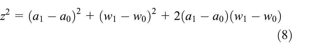
Taking expectations of both sides of equation (8) and realizing that $a_{0}$ and $a_{1}$ are uncorrelated with $w_{0}$ and with $w_{1}$ , we get

\begin{matrix} E [z^{2}] = E [{(a_{1} - a_{0})}^{2}] + E [{(w_{1} - w_{0})}^{2}] \\ + 2 E [(a_{1} - a_{0}) (w_{1} - w_{0})] \\ = E [{(a_{1} - a_{0})}^{2}] + E [{(w_{1} - w_{0})}^{2}] \end{matrix}

(9)

The signal power $E [(a_{1} - a_{0})^{2}]$ will be unaffected as the noise canceller with objective to minimize $E [z^{2}]$ . Accordingly, the minimum output power is

\min E [z^{2}] = E [{(a_{1} - a_{0})}^{2}] + \min E [{(w_{1} - w_{0})}^{2}]

(10)

When $E [z^{2}]$ is minimized, $E [(w_{1} - w_{0})^{2}]$ is, therefore, also minimized. Moreover, when $E [(w_{1} - w_{0})^{2}]$ is minimized, $E [(z - (a_{1} - a_{0}))^{2}]$ is also minimized, since from equation (7)

[z - (a_{1} - a_{0})] = (w_{1} - w_{0})

(11)

From equation (7), the output $z$ will contain the pure signal difference value $Δ a$ plus noise difference value $Δ w$ . The output noise is given by $Δ w = w_{1} - w_{0}$ . Since minimizing $E [z^{2}]$ minimizes $E [(w_{1} - w_{0})^{2}]$ , minimizing the total output power minimizes the output noise power.⁴³

It is seen from equation (8) that the smallest possible output power is $E [z^{2}] = E [(a_{1} - a_{0})^{2}]$ . When this is achievable, $E [(w_{1} - w_{0})^{2}] = 0$ . Therefore, $z = a_{1} - a_{0}$ . In this case, minimizing output power results the output signal to be totally noise free.

Assume a signal is stationary, $x (t + T)$ sampled at $t + T$ is correlated with $x (t)$ sampled at previous time step, as shown in Figure 4. The autocorrelation of signal $x$ sampled with time interval $T$ in discrete time is defined as

R_{xx} (T) = \sum_{t = - \infty}^{\infty} x_{t} x_{t + T}

(12)

Therefore, the power spectral density $S_{xx} (f)$ of the Z-tranform of the autocorrelation $R_{xx} (τ)$ is

S_{xx} (f) = \frac{1}{2 π} \sum_{T = - \infty}^{\infty} R_{xx} (τ) e^{- 2 π jf T}

(13)

where $f$ denotes the spectral component in the frequency domain.

Figure 4.

A signal $x (t)$ is assumed to be stationary. $x (t + T)$ sampled at $t + T$ is correlated with $x (t)$ sampled at previous time step in some way. The autocorrelation of signal $x (t)$ is defined as $R_{xx} (T) = \sum_{t = - \infty}^{\infty} x_{t} x_{t + T}$ .

Thus, in our case, the power spectral density of the input noise sampled with time interval $τ$ is

S_{ww} (f) = \frac{1}{2 π} \sum_{τ = - \infty}^{\infty} R_{ww} (τ) e^{- 2 π jf τ}

(14)

where $R_{ww} (τ)$ is the autocorrelation of the input noise $w_{t}$

R_{ww} (τ) = \sum_{t = - \infty}^{\infty} w_{t} w_{t + τ}

(15)

Our method works for all the correlated noises which is slowly time varying in general. One case is shown in Figures 7 and 8. There is no restriction for the correlation model of the noise, since our analysis is based on the basic definition of the correlation in equation (15).

The output noise at time step $m$ is the difference value of the two neighboring sampled noises, which is designed by our noise canceller

\begin{matrix} w_{{out}_{m}} = w_{m} - w_{m - 1} \\ = w [m τ] - w [m τ - τ] = w_{out} [m τ] \end{matrix}

(16)

Therefore, the relationship between the power spectral density of the output noise and one of the input noises is

S_{w w_{out}} (f) = 2 [1 - \cos (2 π τ f)] S_{ww} (f)

(17)

which is proved in Appendix 1. Hence, the magnitude square of the frequency response of the linear time-invariant (LTI) system in Figure 3 is

| H (f) |^{2} = 2 [1 - \cos (2 π τ f)]

(18)

which is also shown in Figure 5. Because of the inherent periodicity of the discrete time–frequency response, frequencies around $2 π$ are indistinguishable from frequencies around $0$ . Thus, we just take the frequency interval $(- π, π]$ to specify the transfer function of the noise canceller. From Figure 5, we can see that the noise canceller works well in low-frequency region, between the frequency interval $[- π / 3, π / 3]$ when $τ = 1$ .

Figure 5.

The magnitude square of the frequency response of the noise canceller system in Figure 3 ( $τ = 1$ ). The frequency response is periodic with period $2 π$ . Only one period is shown in $(- π, π]$ .

Denoising effectiveness

Assume the noise $w_{i}^{t}$ is combined by

w_{i}^{t} = A_{n_{i}}^{t} + n_{i}^{t}

(19)

where $A_{n_{i}}^{t}$ is the mean value of the noise at time step $t$ , and for each node $i$ , $A_{n_{i}}^{t}$ changes slowly as time step $t$ changes. $n_{i}^{t}$ follows Gaussian distribution, $n_{i}^{t} ~ N (0, σ_{n_{i}^{t}}^{2})$ with zero mean and variance $σ_{n_{i}^{t}}^{2}$ .

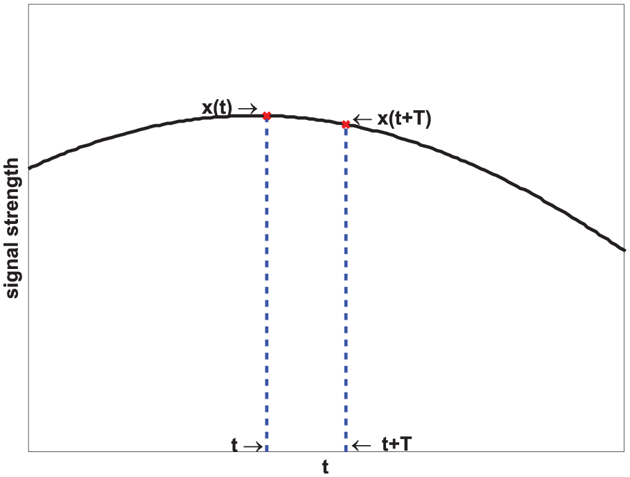
The signal strength curves of one sensor node labeled as $36$ are shown in Figure 6. Its practical received signal strength containing the noise and the theoretical one sampled from the target are shown in Figure 7. The discrepancy between the two curves indicates that the received signal strength involves errors as a distance measurement due to the noise effect.

Figure 6.

The sensor nodes and the target trajectory. The sensor node labeled $36$ is taken for example, and its coordinate $x_{36} = 46.68, y_{36} = 56.77$ .

Figure 7.

The theoretical received signal strength ( $a_{i}^{t}$ ) and the practical one ( $s_{i}^{t}$ ) of the sensor node $36$ ( $P_{0} = 25, 000$ , $A_{n_{36}}^{t} = A_{0} + sl \cdot time step$ , $A_{0} = - 2$ , $sl = 0.05$ , $σ_{n_{36}^{t}} = 0.05$ , $x_{36} = 46.68 m$ , $y_{36} = 56.77 m$ ).

The RSSD values sampled from the sensor node $36$ are shown in Figure 8. The curves show that the practical RSSD values containing noises are very close to the difference values of pure signal strength without noise. Most RSSD values are around zero because at most time steps, the target is far from the node, and the received weak signal strength hardly changes. Only when the target moves close to the sensor node at one point, the RSSD value would increase suddenly. A total of two peak RSSD values, positive or negative, in Figure 8 correspond to the two cases that the target moving close to or moving far away from the sensor node, respectively. Also, in our tracking algorithm, only the RSSD values greater than the threshold $δ$ are kept by the processing node. Others are dropped because their signs are easily disturbed by the noise and untrusted for calculating the estimation region of the target.

Figure 8.

The ideal RSSD values and the practical ones with noises of the sensor node $36$ ( $P_{0} = 25, 000$ , $A_{n_{36}}^{t} = A_{0} + sl \cdot time step$ , $A_{0} = - 2$ , $sl = 0.05$ , $σ_{n_{36}^{t}} = 0.05$ , $x_{36} = 46.68 m$ , $y_{36} = 56.77 m$ ). A total of two peak RSSD values, positive or negative, correspond to the two cases that the target moving close to or moving far away from the sensor node, respectively.

From equations (3) and (19), the received signal strength $s_{i}^{t}$ is combined by

s_{i}^{t} = a_{i}^{t} + A_{n_{i}}^{t} + n_{i}^{t}

(20)

Similarly, for the last time step

s_{i}^{t - 1} = a_{i}^{t - 1} + A_{n_{i}}^{t - 1} + n_{i}^{t - 1}

(21)

By making difference the above two equations, we obtain

s_{i}^{t} - s_{i}^{t - 1} = a_{i}^{t} - a_{i}^{t - 1} + A_{n_{i}}^{t} - A_{n_{i}}^{t - 1} + n_{i}^{t} - n_{i}^{t - 1}

(22)

For both $n_{i}^{t} ~ N (0, σ_{n_{i}^{t}}^{2})$ and $n_{i}^{t - 1} ~ N (0, σ_{n_{i}^{t - 1}}^{2})$

σ_{Δ n_{i}^{t}}^{2} = σ_{n_{i}^{t}}^{2} + σ_{n_{i}^{t - 1}}^{2} - 2 C_{n_{i}^{t} n_{i}^{t - 1}}

(23)

where $Δ n_{i}^{t} = n_{i}^{t} - n_{i}^{t - 1}$ and $C_{n_{i}^{t} n_{i}^{t - 1}}$ is the covariance value of $n_{i}^{t}$ and $n_{i}^{t - 1}$

\begin{matrix} C_{n_{i}^{t} n_{i}^{t - 1}} = E {(n_{i}^{t} - m_{n_{i}^{t}}) (n_{i}^{t - 1} - m_{n_{i}^{t - 1}})} \\ = E {n_{i}^{t} \cdot n_{i}^{t - 1}} \end{matrix}

(24)

because the mean value of both $n_{i}^{t}$ and $n_{i}^{t - 1}$ is zero.

If the noises are highly correlated between the two neighboring sampling time steps and if we choose a pretty small sampling time interval $τ$ , $A_{n_{i}}^{t} \to A_{n_{i}}^{t - 1}$ , and $n_{i}^{t} \to n_{i}^{t - 1}$ . Then, we obtain

σ_{Δ n_{i}^{t}}^{2} \to σ_{n_{i}^{t - 1}}^{2} + σ_{n_{i}^{t - 1}}^{2} - 2 E {{(n_{i}^{t - 1})}^{2}} = 2 σ_{n_{i}^{t - 1}}^{2} - 2 σ_{n_{i}^{t - 1}}^{2} = 0

(25)

The mean square error (MSE) of the estimation of $Δ a_{i}^{t}$ using RSSD value $Δ s_{i}^{t}$ is equal to $σ_{Δ a_{i}^{t}}^{2}$ $σ_{Δ n_{i}^{t}}^{2} / (σ_{Δ a_{i}^{t}}^{2} + σ_{Δ n_{i}^{t}}^{2})$ . If $σ_{Δ n_{i}^{t}}^{2} \to 0$ , $MSE \to 0$ and, therefore, $Δ s_{i}^{t} \to Δ a_{i}^{t}$ . The RSSD value $Δ s_{i}^{t}$ is close enough to the difference value of the pure signal strength $Δ a_{i}^{t}$ .

Threshold denoising

Above noise model is an ideal case that is highly correlated between neighboring sampling time steps. The denoising effectiveness of the noise canceller would not work well for the noise with low correlation. To further reduce the noise effect, a threshold denoising method is introduced, as shown in Figure 3 and equation (6). Figure 3 shows that the output of the noise canceller $z$ is the input of the threshold denoising. By adjusting a reasonable threshold $δ$ defined in equation (6), we could further strengthen the denoising effect of the RSSD method. A total of two indicators are defined to evaluate the threshold denoising effect:

Sign report accuracy is the rate of the sensor nodes whose RSSD sign is the same as the sign of $Δ a_{i}^{t}$ . The sign report accuracy directly decides the localization accuracy of our possible zone, since the possible zone is the intersection part of numerous marginal zones, the opposite sign of RSSD due to the noise disturb will flip the marginal zones from outside to inside, or vice versa, for intersecting, which will directly affect the formation of the possible zone. And as follows, it affects the final estimate position, which is chosen inside the incorrect possible zone. To reduce the probability of the fault sign that occurs, we use the threshold method which is defined in equation (6), and the deterministic approach will be introduced later in this section to filter high-quality RSSD, with positive and relatively large absolute value

S i g n r e p o r t a c c u r a c y = \frac{No . of node i {sign of {RSSD}_{i} = sign of Δ a_{i}}}{No . of node i {| {RSSD}_{i} | > δ}}

(26)

2. Availability is the rate of the sensor nodes whose RSSD absolute values are greater than the threshold $δ$ , which satisfy equation (6), relative to all the sensor nodes

Availability = \frac{No . of node i {| RSS D_{i} | > δ}}{Total no . of nodes}

(27)

Figure 9(a) indicates that a larger threshold $δ$ would boost the sign report accuracy. Since the nodes with small absolute value of RSSD below the threshold $δ$ are dropped, the left nodes with higher RSSD absolute value would report the RSSD sign more reliably, which would increase the sign report accuracy. The RSSD filtered by the threshold has a higher immunization to the noise since the noise hardly changes the sign of an RSSD with a large absolute value. In the meantime, sign report accuracy of the sensor nodes under the noise with a smaller standard deviation will increase faster as the threshold $δ$ increases, as shown in Figure 9(a), since the noise is the fundamental issue that distorts the sign prediction using RSSD. It also means that to achieve the same sign report accuracy under a greater standard deviation noise, a larger threshold $δ$ is needed.

Figure 9.

A higher sign report accuracy is at the cost of less availability of the sensor nodes. A reasonable threshold $δ$ is figured based on the balance of both sign report accuracy and availability. (a) Sign report accuracy of the sensor nodes: Under noise with a certain standard deviation $σ$ value, a higher threshold $δ$ will boost the sign report accuracy. (b) Availability of the sensor nodes: Initially, the availability of the sensor nodes is 100%. As the threshold value increases, the availability of the nodes would be reduced, until going to zero asymptotically.

Figure 9(b) shows that the availability of the sensor nodes is always starting from 100% when choosing a $0$ threshold, whatever the standard deviation $σ$ of the noise is. It is intuitive because $δ = 0$ means that there is requirement for the RSSD in terms of the absolute value. While as the threshold increases, the availability of the nodes will be decreased. Because only the nodes with RSSD absolute value higher than the increased threshold $δ$ are kept. Gradually, the number of available sensor nodes will be close to zero as the threshold $δ$ continually increases.

Although larger threshold $δ$ would boost the sign report accuracy, it would also reduce the availability of the sensor nodes. Since as the threshold $δ$ increased, there were less sensor nodes that satisfy the threshold requirement. Only the sensor nodes with relatively high absolute value of RSSD are left, whose location change relative to the moving target is large enough. While the number of these kinds of sensor nodes is limited. The sign report accuracy and the availability of the nodes need to be balanced by choosing a reasonable threshold. Depending on different values of the standard deviation $σ$ of the noise, a certain threshold is chosen considering both sign report accuracy and availability.

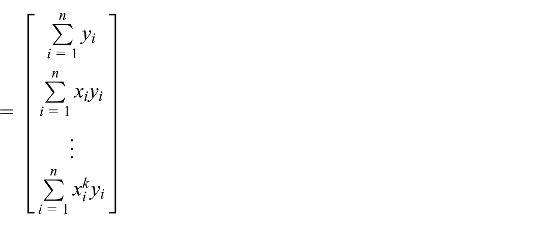
The curves in Figure 9(a) and (b) are gained by averaging the statistics from the whole trajectory. Besides, the locations of sensor nodes are generated randomly and uniformly, and the target trajectory is also generated randomly. Thus, the curves can be referenced to select a threshold. From the following, we will determine the threshold $δ$ : First, the polynomial fitting method is adopted to estimate the curve based on the sampling data points $(x_{i}, y_{i})$ , $i = 1, 2, \dots, n$ , under one specific noise deviation $σ$ . Then, an optimization problem is defined to search an optimal threshold by balancing the two indicators.

A kth degree polynomial is used to estimate the curve based on the $n$ sampling data points

y = c_{0} + c_{1} x + \dots + c_{k} x^{k}

(28)

By substituting $(x, y)$ with actual sampling data points, we obtain the following matrix by a least squares fit

[\begin{matrix} 1 & x_{1} & \dots & x_{1}^{k} \\ 1 & x_{2} & \dots & x_{2}^{k} \\ ⋮ & ⋮ & ⋱ & ⋮ \\ 1 & x_{n} & \dots & x_{n}^{k} \end{matrix}] [\begin{matrix} c_{0} \\ c_{1} \\ ⋮ \\ c_{k} \end{matrix}] = [\begin{matrix} y_{1} \\ y_{2} \\ ⋮ \\ y_{n} \end{matrix}]

(29)

The above equation can be abbreviated as

Xc = y

(30)

Left multiplying both sides by the transpose of $X$ , we obtain

[\begin{matrix} n & \sum_{i = 1}^{n} x_{i} & \dots & \sum_{i = 1}^{n} x_{i}^{k} \\ \sum_{i = 1}^{n} x_{i} & \sum_{i = 1}^{n} x_{i}^{2} & \dots & \sum_{i = 1}^{n} x_{i}^{k + 1} \\ ⋮ & ⋮ & ⋱ & ⋮ \\ \sum_{i = 1}^{n} x_{i}^{k} & \sum_{i = 1}^{n} x_{i}^{k + 1} & \dots & \sum_{i = 1}^{n} x_{i}^{2 k} \end{matrix}] [\begin{matrix} c_{0} \\ c_{1} \\ ⋮ \\ c_{k} \end{matrix}]

= [\begin{matrix} \sum_{i = 1}^{n} y_{i} \\ \sum_{i = 1}^{n} x_{i} y_{i} \\ ⋮ \\ \sum_{i = 1}^{n} x_{i}^{k} y_{i} \end{matrix}]

X^{T} Xc = X^{T} y

(31)

Thus, the polynomial matrix can be achieved by

c = ({X^{T} X)}^{- 1} X^{T} y

(32)

Based on the statistic points from Figure 9, the estimate function of sign report accuracy and availability in terms of the threshold $δ$ can be gained by the above method. We use $E_{1} = f_{1} (δ)$ and $E_{2} = f_{2} (δ)$ to denote the functions of two indicators sign report accuracy and availability, respectively. An optimization problem is defined as follows to find an optimal threshold $δ$

\begin{matrix} \underset{δ, σ_{i}}{maximize} & E_{1} \\ subject to & E_{2} \geq ava_toler \\ σ = σ_{i} \end{matrix}

(33)

where $ava_toler$ is the tolerable minimum value of the availability of the sensor nodes and $σ_{i}$ is the specific noise deviation value.

RSSD-based tracking estimation method

In this section, a practical method is provided to track an arbitrary moving target in WSNs based on the RSSD. Different from RSSI, RSSD is not to give the location of target by means of calculating the absolute distances between target and nodes but to determine the location by estimating the most possible location with the change in RSSI. The estimation process is divided into three stages, the possible zone, the refined zone, and the final location. Along with the process, the possible range of the target is gradually narrowed down to a certain point. The following subsections will give the details of the method.

The possible zone

The definition

A possible zone is regarded as the estimated geometric range which limits the real position of the target at a certain time and is able to provide an accurate location range of the target just by using the sign of RSSD. The possible zone can be further defined as the intersection area of all the available sensor nodes’marginal zones. All available nodes’ RSSD values will be processed by the processing node to estimate the possible zone. The possible zone of the target at time step $t$ is calculated by

p z_{t} = ⋂_{i = 1}^{n_{t}} c_{i, t}^{sig ({RSSD}_{i}^{t})}

(34)

where $n_{t}$ is the number of available sensor nodes at time step $t$ and $⋂_{i = 1}^{n_{t}}$ denotes the intersection of the marginal zones of the $n_{t}$ sensor nodes.

Because the intersection of marginal zones is generally not a regular shape, the range of the possible zone is greatly difficult for us to determine by plane geometry, particularly as there are a large number of marginal zones of the sensor nodes. To simplify the problem, we adopt a set of points deployed uniformly with a certain density in the range of the zone to characterize the size of the area. The possible zone at time step $t = 24$ composed of a set of black reference dots is shown in Figure 10. The reference dots are the points uniformly distributed in the reference coordinates with a certain density. We only draw the reference dots inside the possible zone. (The dots on the zone boundary are also drawn.)

Figure 10.

The possible zone in a set of black reference dots. The example is at time step $t = 24$ . The black reference dots are distributed with a density of $0.5 m$ in the range of the zone. The purple line is the boundary of the estimated possible zone, connected by the outermost black reference dots.

Optimizing processing

Although the set of points can effectively reduce the computational load, in practical calculation, massive and frequent processing still tackles the efficiency of determining the possible zone’s range. Before obtaining the final possible zone, the range could be gradually shrunk as more marginal zones intersect together in a random order. Although the determination of the possible zone practically runs in PC, which is linked to the sink node, the computational efficiency is also needed to be considered. For ensuring the real-time tracking to the greatest extent, we should simplify the original calculation process in terms of how to choose a more effective order to intersect the marginal zones down to the possible zone.

Scheduling a reasonable intersection order of the marginal zones is effective to promote the convergence rate of the possible zone. Intuitively, starting the intersection with a small marginal zone, the possible zone could be narrowed down immediately. However, if the intersection starts with one greatly large zone, it is possible that the range shrinks very slowly at first and then suddenly narrows down as meeting a small marginal zone. An order-selection mechanism is proposed: intersect the zones by ascending order of zone radius, choosing the smallest marginal zones first. Here, we only adopt the nodes with 1 zones, which we will explain in detail. As shown in Figure 11, the zone bounded in purple line is the possible zone, and the zones inside the red marginal circles are starting zones which participates in the intersection process first. As we can see, choosing the smallest zone first could be tremendously beneficial for intersection range converging than choosing a larger zone randomly.

Figure 11.

The starting zones for the intersection when the target is at time step $t = 24$ . The zone bounded by the purple line is the possible zone. The zones bounded by the red marginal circles are the starting zones to participate in the intersection process first. A total of two choices show the advantage of choosing the starting zone with the smallest radius: (a) choosing the smallest zone and (b) choosing a larger zone randomly.

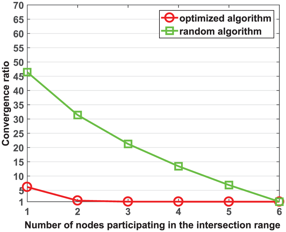
The comparison of the convergence ratio between the optimized algorithm by order of the zone radius and the original algorithm by choosing the nodes randomly, at time step $24$ , is shown in Figure 12. The ratio curves show that the optimized algorithm converges to the possible zone using only three sensor nodes. While the original algorithm does not converge to the possible zone until using all of the six available sensor nodes’ 1 zones. Therefore, we calculate equation (35) by the ascending order of the 1 zones’ radius to accelerate the intersection process.

Figure 12.

The comparison of the convergence ratio between the optimized algorithm and the original algorithm. The example is at time step $24$ , when there exist six sensor nodes with 1 zones. The intersection range using the optimized algorithm by ascending order of the zone radius converged faster than using the original algorithm by intersecting the zones randomly. The random intersection order is generated by the initial array sequence of the sensor nodes that has not been sorted by order of zone radius. We reconsider all the random cases, and each case is one specific order of the permutation of the six sensor nodes. So, there are $6! = 6 \times 5 \times 4 \times 3 \times 2 \times 1 = 720$ cases in total. Since each case has the same probability of happening, we average the convergence ratio on each case.

Intuitively, the 0 zone has greater area than the 1 zone with the same zone radius, though this inference is not rigorous enough. It provides a potential scheme to simplify the calculation procedure, to intersect only 1 zones instead of all marginal zones, and equation (34) can be simplified as below

p z_{t} = ⋂_{i = 1}^{{n'}_{t}} c_{i, t}^{1}, ({n'}_{t} \leq n_{t})

(35)

where only the nodes with 1 zones participate in the intersection computing and $n'_{t}$ is the number of nodes having 1 zones, instead of using all $n_{t}$ available sensor nodes.

To prove the above inference feasible, we compare two convergence ratios, which are calculated by the intersection ranges contributed by 0 zones and 1 zones, respectively, divided by the area of possible zone. The convergence ratios at different time steps are shown in Figure 13, which indicates that the area contributed by 1 zones is extremely smaller than the area contributed by 0 zones at almost all time steps. Thus, the 1 zone definitely converges more efficiently than the 0 zone. The nodes with 0 zones or negative RSSD values will be dropped from the intersection list.

Figure 13.

The convergence ratios of 1 zones’ and 0 zones’ intersection range. The convergence ratio is greater or equal to $1$ , which is calculated by the area of intersection range divided by the area of the possible zone. The convergence ratio of the intersection range contributed by the 1 zones is extremely smaller than the one contributed by the 0 zones.

Terminal condition

The intersection range converges finally when its area is equal or approximately equal to the final possible zone (this final possible zone has eliminated the 0 zones’ contribution, and we can tolerate the intersection range a little bit greater than the exact final possible zone, for instance, 5% greater, since it is reasonable to use less sensor nodes participating in the intersection process than actual total available sensor nodes). After the calculation for some time, the more the sensor nodes are picked, the slower the convergence rate of the intersection range occurs, as shown on the red curve in Figure 12. Although the computational processing of the possible zone has been optimized by the ascending order of 1 zones’ radii, there still exist some 1 zones with large radii that make little or even no contribution to the possible zone in the last period of intersection. Since we have almost used up small zones, the large zones left are not significant to the convergence of the final zone. These large zones also need to be dropped to reduce computational redundancy. To achieve this goal, one area change ratio $R_{ac}$ is defined as our terminal condition for intersection

R_{ac} = \frac{| S (⋂_{i = 1}^{n_{\max}} c_{i, t}^{1}) - S (⋂_{i = 1}^{n_{\max}^{- 1}} c_{i, t}^{1}) |}{S (⋂_{i = 1}^{n_{\max}^{- 1}} c_{i, t}^{1})} \leq ε, (1 \leq n_{\max} \leq {n'}_{t})

(36)

where $S (\cdot)$ denotes the area of the intersection range, $n_{\max}$ denotes the index number of the last node participating in the intersection, and $ε$ is a threshold value as a stopping condition: If the area change ratio $R_{ac}$ is smaller than the threshold value $ε$ after using the node $n_{\max}$ , the intersection process is forced to stop, and the subsequent $n'_{t} - n_{\max}$ nodes are dropped. Finally, the optimal possible zone is obtained.

Overall, we analyze the algorithm complexity of the optimizing processing for getting the possible zone. We conclude that the computational complexity of the optimized algorithm is always less than the original one. For the original algorithm without the order-selection mechanism, since it gains the possible zone by intersecting all available sensor nodes’marginal zones without reservation, which takes $O (n)$ . And also, the intersecting computation will take the total number of reference dots in all of the marginal zones, which is denoted as $O (N)$ , because comparison work needs to be done to find the common dots of marginal zones by intersecting each one. Thus, the total complexity of the original algorithm is $O (n + N)$ . While the optimized algorithm sorts the sensor nodes by order of their zone radius, and we use a linear time-sorting algorithm, which takes $O (n)$ time. And the total number of reference dots for computing is reduced because less nodes will be used for intersection after we delete the nodes with RSSD value decreased. Thus, the optimized algorithm takes $O (n + N')$ time totally, where $N' < N$ , and $N >> n$ , $N' >> n$ . Moreover, the optimized algorithm definitely converges faster than the original one, since we intersect the zones with their radius priority.

The refined zone

The possible zone is determined by the sign of RSSD, and it has been proved that the target is certainly located within the possible zone. While the area of possible zone might be still large if there were not enough sensor nodes near the target. The case is difficult for us to choose the location point in the zone. In this section, we will further shrink the zone using the absolute value of RSSD if the possible zone is not small enough.

In Figure 14, $r_{i} (t - 1)$ is the distance between node $i$ and the target at last time step $t - 1$ . $r_{i} (t)$ is the distance between node $i$ and the target at current time step $t$ , which is unknown. $r_{i} (t)$ can be estimated based on RSSD value and the distance $r_{i} (t - 1)$ at previous time step. We would not estimate the distance $r_{i} (t)$ based on the RSSI, since we wish to reduce the measurement error due to RSSI.

Figure 14.

The distance $r_{i} (t)$ between node $i$ and the target at current time step $t$ is estimated by the distance $r_{i} (t - 1)$ at previous time step and the absolute value of RSSD.

The distance $r_{i} (t)$ between node $i$ and the target is calculated by the following

{\hat{s}}_{i}^{t} = {\hat{a}}_{i}^{t - 1} + {RSSD}_{i}^{t}

(37)

where ${\hat{a}}_{i}^{t - 1} = P_{0} / {\hat{r}}_{i}^{2} (t - 1)$ and ${\hat{r}}_{i} (t - 1) = ∥ {\hat{q}}_{t - 1} - {[x_{i}, y_{i}]}^{T} ∥_{2}$ .

The estimated distance ${\hat{r}}_{i} (t)$ can be solved by

{\hat{r}}_{i} (t) = a^{- 1} ({\hat{s}}_{i}^{t})

(38)

where $a^{- 1} (\cdot)$ is the inverse function of $a (\cdot)$ defined by equation (2).

The refined zone is the intersection region of circles formed by each node position $[x_{i}, y_{i}]^{T}$ and the estimated distance $r_{i} (t)$ , as shown in Figure 15. In general, if there exist two more nodes available to draw the circles, the possible zone can be further shrunk to an interior intersection region of these circles, as shown in Figure 15(a). While if there does not exist at least two nodes, the circles may not form a closing intersection region. In this case, the boundaries of the possible zone can serve as complementary peripheries (the purple line) of the refined zone, as shown in Figure 15(b).

Figure 15.

The possible zone is further shrunk to the refined zone (the yellow shadow region). A total of two cases are considered: (a) two more nodes and (b) fewer nodes.

The final location

The possible zone has been shrunk to the refined zone, which is small enough for further positioning. The set of reference dots distributed with a certain density in the refined zone will be utilized to calculate the final location, by the aid of a norm function. Positioning with the reference dots will also compensate the localization inaccuracy of the previous zones.

The final location of the target is substituted by the location of the reference dot in the refined zone with the minimum norm

\underset{j}{\arg min} {(\sum_{i = 1}^{n_{t}} | s_{i}^{t} - a_{ij}^{t} |^{2})}^{1 / 2}

(38)

where $s_{i}^{t}$ is the measured RSSI value on node $i$ received from the target, $a_{ij}^{t}$ is the theoretical RSSI value on node $i$ from the reference dot $j$ , and $n_{t}$ is the total available number of sensor nodes at this time step. The estimated location of the target at current time step ${\hat{q}}_{t}$ is the location of the reference dot $j$ with the minimum norm value.

Simulation results

In this section, the performance of the proposed RSSD-based localization algorithm is compared with the RSSI-based method. The purpose of this analysis is to show how the two algorithms’ localization error is affected by noise. For the RSSD-based method, we also present how the localization accuracy is affected by setting different threshold $δ$ and the reference dot density. Besides, we show how much the area of the zone could be shrunk from the possible zone to the refined zone. Finally, we compare the computational time between the original algorithm and the optimized algorithm to make the possible zone.

In simulation experiment, one sensing field of area $100 m \times 100 m$ is considered, in which $50$ sensor nodes are deployed randomly and uniformly. One single target is moving through the area, and its velocity magnitude and direction are generated randomly at each time step $t = 1, 2, \dots, N$ .

The impact of noise

The average localization errors of the RSSI-based method and the RSSD-based method are shown in Figure 16. The localization error is calculated under different standard deviation $σ$ of the noise from $0.01$ to $1.0$ , to verify the two algorithms’ robustness to the impact of noise. For the RSSI-based method, we adopt the trilateration algorithm: The estimated distance based on the strength of received signal is used to draw the circles with center located at the three reference sensor nodes.⁴⁴ Ideally, the intersection point of the three circles should be the target’s location. However, due to the noise effect, there could exist more than one intersection or does not exist intersection at all. If there is no intersection, we should enlarge the circles simultaneously until they intersect each other. If there exists more than one intersection between two sensor nodes’ circles, the nearest intersection to the third node is chosen as the target’s location.⁴⁵ From Figure 16, we can observe that the RSSI-based method could perform well under the noise with deviation, and the error even goes slightly lower coincidentally as the deviation $σ$ increases. While the localization error starts to boost rapidly when $σ$ value is larger than $0.4$ . Subsequently, the localization error continues to grow. As a result, the RSSI-based method will lose its localization effectiveness under the noise with large variance. In contrast, the localization error of the RSSD-based method grows slightly as the noise’s deviation increases. There exists a little oscillations when $σ$ becomes larger. While the RSSD-based method performs definitely more stably than RSSI. Thus, the RSSD-based algorithm is more robust to the noise effect.

Figure 16.

The localization error of the RSSI-based method and the RSSD-based method. A trilateration algorithm is adopted based on the RSSI method of distance estimate.

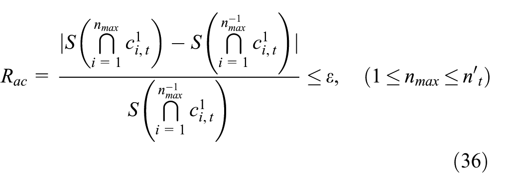
The impact of threshold

The performance of the RSSD-based method in terms of different threshold $δ$ is shown in Figure 17. The average localization error is reduced rapidly as the threshold $δ$ increases from $0$ to $0.5$ with small standard deviation $σ$ , as shown in Figure 17(a). As mentioned, the increasing threshold would reduce the probability of false sign report of the RSSD. The correctness of sign report guarantees the intersection process of marginal zones going well. For the standard deviation larger than 0.5, we start sampling $δ$ from $0.5$ , otherwise the algorithm would go wrong using smaller threshold. In general, after the threshold $δ$ increases to a certain value, the localization error will not be reduced anymore, but flat to a certain value. This is because as $δ$ exceeds the value that is enough to guarantee the correctness of the sign report for a certain noise, the localization error will not be affected by the threshold. On the contrary, an overlarge threshold is disadvantageous for the algorithm to choose the final location in the enlarged zone due to the reduced number of sensor nodes providing information. In Figure 17(b), as the threshold increases, the number of reference dots or the area of the refined zone would reduce first and ascend slowly and then approach to a certain value. Initially, the number of reference dots decreases because the correctness of the RSSD sign report would boost as the threshold value increases, which guarantees the possible zone is converged to a certain area. As the threshold continuously is on the rise, more sensor nodes will be invalid and the zone area would be expanded. However, the computational complexity of the reference dot selection for the target’s final location is linear to the number of reference dots in the zone area, $O (N)$ .

Figure 17.

The performance of the RSSD-based method in terms of the threshold value $δ$ . The reference dot density (the distance between the two neighboring reference dots in the zone) is $0.5 m$ : (a) the localization error of the RSSD based and (b) the average number of reference dots in the refined zone. As the standard deviation of the noise becomes larger, there would be more uncertainty for the localization, which causes the fluctuation. For example, the purple curve with the largest standard deviation $σ$ shown in this figure has a larger fluctuation range than the other cases.

The impact of reference dot density

Both localization accuracy and calculation workload take into account another parameter, the reference dot density (the distance between the two neighboring reference dots). From Figure 18, the average localization error grows slightly as the reference dot density becomes sparse in the zone. A high reference dot density boosts the accuracy slightly, whereas it greatly enlarges the computational amount greatly as well. There could be nearly $8000$ reference dots when the reference dot density value is $0.1 m$ . For the sake of the reduction of the computational amount, the accuracy will inevitably be not as high as required. For instance, with the value of reference dot density $0.5 m$ , the localization error will not increase too much compared with the value of $0.1 m$ , but the number of reference dots would be extremely reduced.

Figure 18.

(a) The average localization error is related to the reference dot density and (b) the number of reference dots in the refined zone in terms of the reference dot density.

The comparison of area

The comparison of the area of the possible zone and the refined zone is shown in Figure 19. The possible zone is the intersection part of 1 zones of active sensor nodes. While at some time steps, there may be few sensor nodes near the target. Thus, the area of the possible zone may be relatively large under this poor condition. The refined zone is extremely narrowed down from the possible zone, as shown in Figure 19(a), which definitely enhances the calculation efficiency. One case of the possible zone and the refined zone of the target at time step $24$ is shown in Figure 19(b).

Figure 19.

The area of the possible zone and the refined zone at each time step. The reference dot density is $0.5 m$ . The noise deviation value is $σ = 0.5$ . Accordingly, the threshold value is chosen as $δ = 2.0$ for making the possible zone: (a) the possible zone and the refined zone at time step $24$ and (b) the number of reference dots in each zone at each time step.

The comparison of computational expense

Finally, the comparison of the computational time (s) between the original and the optimized algorithms for making the possible zone is shown in Figure 20. The result presents that the computational time is immensely compressed by our optimization: The nodes with negative RSSD values owning 0 zones are removed from the intersection list, and the intersection process is ordered by the zone radius so that the intersection range can be narrowed down as soon as possible. Due to the optimization, the intersection range of the target is converged in advance. Therefore, the optimized algorithm extremely reduces the calculation time for the possible zone.

Figure 20.

The comparison of computational time between the original and the optimized possible zone algorithm. The test is executed by MATLAB R2014a on Mac.

Conclusion

In this article, we propose a new target tracking method based on the RSSD, which is available for all kinds of moving targets. By making difference value of the received signal strengths sampled from two neighboring time steps, the influence of noise on the estimation can be reduced. Based on the sign of RSSD, one possible zone of the target is estimated. Then, we optimized the intersection algorithm to reduce the computational time. We further shrink the possible zone to the refined zone, which is small enough for us to find the target’s location in the zone.

Simulation results show that the noise affects our localization technique slightly. The RSSD-based algorithm is more robust to the noise. The performance of our scheme under various parameters is also provided to evaluate. We analyze the dual characters of the threshold value $δ$ : An increasing threshold $δ$ can boost the localization accuracy, while it can also reduce the number of available sensor nodes, which slows down the zone convergence. The choice of the reference dot density is also considered based on both the localization accuracy and the computational amount. In conclusion, our proposed RSSD-based localization algorithm achieves higher localization accuracy and is robust to the disturbance of the noise with different variance values.

Footnotes

Appendix 1

The output noise of the noise canceller is the difference value of the input noises sampled from the two neighboring time steps with time interval $τ$

(39)

w_{ou t_{m}} = w_{m} - w_{m - 1} = w [m τ] - w [m τ - τ] = w_{out} [m τ]

The autocorrelation of the output noise with time interval $ν$ is

(40)

R_{w w_{out}} (ν) = \sum_{m = - \infty}^{\infty} w_{out} [m τ] w_{out} [ν + m τ]

Substitute equation (40) into equation (13), the power spectral density of the output noise is

(41)

\begin{matrix} S_{w w_{out}} (f) = \frac{1}{2 π} \sum_{ν = - \infty}^{\infty} R_{w w_{out}} (f) e^{- 2 π jf ν} \\ = \frac{1}{2 π} \sum_{ν = - \infty}^{\infty} \sum_{m = - \infty}^{\infty} w_{out} [m τ] w_{out} [ν + m τ] e^{- 2 π jf ν} \end{matrix}

Substitute equation (39) into equation (41), we obtain

(42)

\begin{matrix} S_{w w_{out}} (f) = \frac{1}{2 π} \sum_{ν = - \infty}^{\infty} \sum_{m = - \infty}^{\infty} {w [m τ] - w [m τ - τ]} \\ \cdot {w [ν + m τ] - w [ν + m τ - τ]} e^{- 2 π jf ν} \end{matrix}

There exist four terms of the product of noises sampled at their corresponding time steps when we expand equation (42)

(43)

\begin{matrix} S_{w w_{out}} (f) = \frac{1}{2 π} \sum_{ν = - \infty}^{\infty} \sum_{m = - \infty}^{\infty} w [m τ] \cdot w [ν + m τ] e^{- 2 π jf ν} \\ - \frac{1}{2 π} \sum_{ν = - \infty}^{\infty} \sum_{m = - \infty}^{\infty} w [m τ] \cdot w [ν + m τ - τ] e^{- 2 π jf ν} \\ - \frac{1}{2 π} \sum_{ν = - \infty}^{\infty} \sum_{m = - \infty}^{\infty} w [m τ - τ] \cdot w [ν + m τ] e^{- 2 π jf ν} \\ + \frac{1}{2 π} \sum_{ν = - \infty}^{\infty} \sum_{m = - \infty}^{\infty} w [m τ - τ] \cdot w [ν + m τ - τ] e^{- 2 π jf ν} \end{matrix}

Rearranging the exponential terms, we obtain

(44)

\begin{matrix} S_{w w_{out}} (f) = \frac{1}{2 π} \sum_{ν = - \infty}^{\infty} \sum_{m = - \infty}^{\infty} w [m τ] \cdot w [ν + m τ] e^{- 2 π jf ν} \\ - \frac{1}{2 π} \sum_{ν = - \infty}^{\infty} \sum_{m = - \infty}^{\infty} w [m τ] \cdot w [ν + m τ - τ] e^{- 2 π j τ f} \cdot e^{- 2 π jf (ν - τ)} \\ - \frac{1}{2 π} \sum_{ν = - \infty}^{\infty} \sum_{m = - \infty}^{\infty} w [m τ - τ] \cdot w [ν + m τ] e^{2 π j τ f} \cdot e^{- 2 π jf (ν + τ)} \\ + \frac{1}{2 π} \sum_{ν = - \infty}^{\infty} \sum_{m = - \infty}^{\infty} w [m τ - τ] \cdot w [ν + m τ - τ] e^{- 2 π jf ν} \end{matrix}

Comparing the coefficients with equation (14), it becomes

(45)

\begin{matrix} S_{{ww}_{out}} (f) = S_{ww} (f) - e^{- 2 π j τ f} S_{ww} (f) - e^{2 π j τ f} S_{ww} (f) + S_{ww} (f) \\ = (2 - e^{-} 2 π j τ f - e^{2} π j τ f) S_{ww} (f) \\ = 2 [1 - \cos (2 π τ f)] S_{ww} (f) \end{matrix}

Acknowledgements

We thank Randy Freeman, Chung-Chien Lee, and Goce Trajcevski (EECS Department, Northwestern University, Evanston, IL) for their valuable suggestions in relation to this work.

Handling Editor: Luca Reggiani

Declaration of conflicting interests

The author(s) declared no potential conflicts of interest with respect to the research, authorship, and/or publication of this article.

Funding

The author(s) disclosed receipt of the following financial support for the research, authorship, and/or publication of this article: This work was supported by National Natural Science Foundation of China (61471110 and U1713216), National Key Research and Development Program of China (2016 YFB0701100 and 2017YFB1300900), Chinese Universities Scientific Foundation (N160208001 and N162 60004), Dr research fund of Liaoning Province (201705 20211) and Shenyang Research Fund (17-87-0-00).

References

Akyildiz

Sankarasubramaniam

et al . Wireless sensor networks: a survey. Comput Netw 2002; 38(4): 393–422.

Zhang

Sun

Song

et al . Ubiquitous WSN for healthcare: recent advances and future prospects. IEEE Internet Things 2014; 1(4): 311–318.

Han

Lee

Crespi

Semantic context-aware service composition for building automation system. IEEE T Ind Inform 2014; 10(1): 752–761.

Murtaza

Kanhere

Ignjatovic

et al . Trajectory approximation for resource constrained mobile sensor networks. In: IEEE international conference on distributed computing in sensor systems, Marina Del Rey, CA, 26–28 May 2014, pp.59–66. New York: IEEE.

Anthony

Bennett

Vuran

et al . Sensing through the continent: towards monitoring migratory birds using cellular sensor networks. In: Proceedings of the 11th international conference on information processing in sensor networks, Beijing, China, 16–20 April 2012, pp.329–340. New York: ACM.

Dyo

Ellwood

Macdonald

et al . Evolution and sustainability of a wildlife monitoring sensor network. In: Proceedings of the 8th ACM conference on embedded networked sensor systems, Zürich, 3–5 November 2010, pp.127–140. New York: ACM.

Olfati-Saber

Jalalkamali

Collaborative target tracking using distributed Kalman filtering on mobile sensor networks. In: Proceedings of the American control conference, San Francisco, CA, 29 June–1 July, pp.1100–1105. New York: IEEE.

Martin

Farrell

Aspey

et al . A high-resolution sensor network for monitoring glacier dynamics. IEEE Sens J 2014; 14(11): 3926–3931.

Pang

Hong

Yao

et al . Design and implementation of a smart mini-base station for the internet of things. In: Asia-pacific microwave conference (APMC), Nanjing, China, 6–9 December 2015, vol. 3, pp.1–3. New York: IEEE.

10.

Patil

Chapalkar

Dhamne

et al . Monitoring system for prisoner with GPS using wireless sensor network (WSN). Int J Comput Appl 201491(13): 28–31.

11.

Niculescu

Nath

Ad hoc positioning system (APS) using AOA. In: IEEE societies twenty-second annual joint conference of the IEEE computer and communications, San Francisco, CA, 30 March–3 April 2003, vol. 3, pp.1734–1743. New York: IEEE.

12.

Wang

Ghosh

Das

SK.

A survey on sensor localization. J Control Theory Appl 2010; 8(1): 2–11.

13.

Niculescu

Nath

DV based positioning in ad hoc networks. Telecommun Syst 2003; 22(1–4): 267–280.

14.

Boukerche

Oliveira

HABF

Nakamura

. Localization systems for wireless sensor networks. IEEE Wirel Commun 2007; 14(6): 6–12.

15.

Niu

Varshney

PK.

Target location estimation in sensor networks with quantized data. IEEE T Signal Proces 2006; 54(12): 4519–4528.

16.

Savvides

Han

Strivastava

MB.

Dynamic fine-grained localization in ad-hoc networks of sensors. In: Proceedings of the 7th annual international conference on mobile computing and networking, Rome, 16–21 July 2001, pp.166–179. New York: ACM.

17.

Whitehouse

Culler

Calibration as parameter estimation in sensor networks. In: Proceedings of the 1st ACM international workshop on wireless sensor networks and applications, Atlanta, GA, 28 September 2002, pp.59–67. New York: ACM.

18.

Hofmann-Wellenhof

Lichtenegger

Collins

et al . GPS-global positioning system: theory and practice. Wien: Springer, 1997.

19.

Wei

Wang

Wan

. A new localization technique based on network TDOA information. In: 6th international conference on ITS telecommunications, Chengdu, China, 21–23 June 2006, pp.127–130. New York: IEEE.

20.

Priyantha

Miu

AKL

Balakrishnan

et al . The cricket compass for context-aware mobile applications. In Proceedings of the 7th annual international conference on mobile computing and networking, Rome, 16–21 July 2001, pp.1–14. New York: ACM.

21.

Mao

Fidan

Anderson

BDO

Wireless sensor network localization techniques. Comput Netw 2007; 51(10): 2529–2553.

22.

Heurtefeux

Valois

Is RSSI a good choice for localization in wireless sensor network? In: IEEE 26th international conference on advanced information networking and applications, Fukuoka, Japan, 26–29 March 2012, pp.732–739. New York: IEEE.

23.

Hofmann-Wellenhof

Lichtenegger

Collins

Global positioning system: theory and practice. Berlin: Springer, 2012.

24.

Liu

Zhang

A locality-based range-free localization algorithm for anisotropic wireless sensor networks. Telecommun Syst 2016; 62(1): 3–13.

25.

Khalid

Gulliver

AA.

Range-based localization in wireless networks using density-based outlier detection. Wirel Sens Netw 2010; 2(11): 807.

26.

Doherty

Pister

KSJ

El Ghaoui

Convex position estimation in wireless sensor networks. In: Twentieth annual joint conference of the IEEE computer and communications societies, Anchorage, AK, 22–26 April 2001, vol. 3, pp.1655–1663. New York: IEEE.

27.

Gui

Val

Wei

et al . Improvement of range-free localization technology by a novel DV-hop protocol in wireless sensor networks. Ad Hoc Netw 2015; 24: 55–73.

28.

Bulusu

Heidemann

Estrin

GPS-less low-cost outdoor localization for very small devices. IEEE Pers Commun 2000; 7(5): 28–34.

29.

Huang

Blum

et al . Range-free localization schemes for large scale sensor networks. In Proceedings of the 9th annual international conference on mobile computing and networking, San Diego, CA, 14–19September2003, pp.81–95. New York: ACM.

30.

Zha

Sensor positioning in wireless ad-hoc sensor networks using multidimensional scaling. In: Twenty-third annual joint conference of the IEEE computer and communications societies, Hong Kong, China, 7–11 March 2004, vol. 4, pp.2652–2661. New York: IEEE.

31.

Woo

Lee

Range-free localization with isotropic distance scaling in wireless sensor networks. In: International conference on information networking, Bangkok, Thailand, 28–30 January2013, pp.632–636. New York: IEEE.

32.

Woo

Lee

Reliable anchor node based range-free localization algorithm in anisotropic wireless sensor networks. In: International conference on information networking, Bangkok, Thailand, 28–30 January 2013, pp.618–622. New York: IEEE.

33.

Joo

Wang

et al . Range-free wireless sensor networks localization based on hop-count quantization. Telecommun Syst 2012; 50(3): 199–213.

34.

Jiang

Lin

et al . ALRD: AoA localization with RSSI differences of directional antennas for wireless sensor networks. In: International conference on information society (i-Society), London, 25–28 June 2012, pp.304–309. New York: IEEE.

35.

Wang

Chen

Lin

et al . High-precision RSSI-based indoor localization using a transmission power adjustment strategy for wireless sensor networks. In: IEEE 14th international conference on high performance computing and communication & IEEE 9th international conference on embedded software and systems (HPCC-ICESS), Liverpool, 25–27 June 2012, pp.1634–1638. New York: IEEE.

36.

Sahu

Sahoo

DuRT: dual RSSI trend based localization for wireless sensor networks. IEEE Sens J 2013; 13(8): 3115–3123.

37.

Zou

Lin

Blind RSSD-based indoor localization with confidence calibration and energy control. Sensors 2016; 16(6): 788.

38.

Gerok

Peissig

Kaiser

TDOA assisted RSSD localization in UWB. In: 9th workshop on positioning navigation and communication, Dresden, 15–16 March 2012, pp.196–200. New York: IEEE.

39.

Friis

HT.

A note on a simple transmission formula. Proc IRE 1946; 34(5): 254–256.

40.

Huang

Barralet

Sharma

Accuracy of location identification with antenna polarization on RSSI. In: Proceedings of the international multiconference of engineers and computer scientists, Hong Kong, China, 18–20 March 2009, vol. 1. New York: IEEE.

41.

Reggiani

Fiorina

Gezici

et al . Radio context awareness and applications. J Sens 2013; 2013: 491092.

42.

Bourges

Guinvarc’h

Uguen

et al . High-frequency surface wave radar based on a sea floating antenna concept. IET Microwaves Antennas Propag 2009; 3(8): 1237–1244.

43.

Widrow

Glover

McCool

et al . Adaptive noise cancelling: principles and applications. Proc IEEE 1975; 63(12): 1692–1716.

44.

Goldoni

Savioli

Risi

et al . Experimental analysis of RSSI-based indoor localization with IEEE 802.15.4. In: European wireless conference (EW), Lucca, 12–15 April 2010, pp.71–77. New York: IEEE.

45.

Kuruoglu

Erol

Oktug

Localization in wireless sensor networks with range measurement errors. In: Fifth advanced international conference on telecommunications, Venice, 24–28 May 2009, pp.261–266. New York.

Received signal strength difference–based tracking estimation method for arbitrarily moving target in wireless sensor networks

Abstract

Keywords

Introduction

Related work

System overview

The target and WSNs

Definition 1 (marginal circle)

Definition 2 (marginal zone)

The measurement

RSSI

RSSD

RSSD-based noise canceller

Denoising effectiveness

Threshold denoising

RSSD-based tracking estimation method

The possible zone

The definition

Optimizing processing

Terminal condition

The refined zone

The final location

Simulation results

The impact of noise

The impact of threshold

The impact of reference dot density

The comparison of area

The comparison of computational expense

Conclusion

Footnotes

Appendix 1

Acknowledgements

Declaration of conflicting interests

Funding

References