Sage Journals: Discover world-class research

Abstract

The location of sensors represents a relevant attribute in wireless sensor networks. In this article, we propose a distributed range-based localization algorithm for wireless sensor network. The algorithm is mainly based on an adaptively local circular searching area where each unknown sensor must find inside a position that minimizes the error distance with neighboring sensors using a local function. The new position of a sensor is broadcast to neighboring sensors allowing collaboratively to other sensors re-estimate their new positions. The iterative process is repeated until a stopping criterion is reached. The performance of the proposed algorithm is evaluated and compared with other state-of-the-art algorithms, and results indicate that the approach overcomes the other methods in both accuracy and time of convergence.

Keywords

Wireless sensor network localization received signal strength

Introduction

A wireless sensor network (WSN) is a network of small sensors that are wirelessly interconnected with each other.¹ The main purpose of the network is monitoring any desired physical or chemical phenomenon. Due to the huge advance in electronic technology, extensive quantities can be measured by sensors. Thus, the use of sensor networks can span different applications, ranging from industry and agriculture, even to health care.²

One of the main requirements to install a WSN is that each sensor knows three elementary sensors information, which are measured quantity, time of measurement, and geographic position. Moreover, each sensor must meet some requirements, such as having the ability to process information and transmit it to another sensor. In addition, the sensor needs to be small and economic and use the smallest amount of energy. The number of sensors used in a WSN can range from hundreds to thousands units, causing an economic issue in the WSN and therefore an increase in the overall network cost.

As a consequence, sensors location has a huge impact on WSN final cost. One possible solution is the use of a Global Positioning System (GPS); however, this is very expensive.³ Another solution is to program the position to every sensor in the network, but this can be a difficult task when the number of the sensors is large.

Because of the above, different algorithms that use fewer sensors with GPS (known as anchors) had been developed. The anchors communicate their position to adjacent sensors which do not know their position (known as unknown sensors), so each of the sensors can estimate their own position indirectly. In order to do so, different techniques and algorithms are used, where the sensor positions can be estimated by distance or proximity techniques.^4–6

Each of the techniques used to estimate distances has different error rates in the distance measurement.^7,8 For instance, no measurement is accurate due to several aspects, such as sensor’s manufacture, power supply, technology used, and environment where the network was deployed. Also obstructions and noise that may be in the system can affect the measurement. This is why a new algorithm that minimizes errors in the estimated positions of unknown sensors is needed.

In this article, we propose an iterative range-based localization algorithm with an adaptive search region. The algorithm is characterized by an adaptive circular search area that proposes a set of possible solutions to reduce the error using a local minimizing function. In the process, each sensor should estimate its own new position and broadcast it to its neighbor sensors. To evaluate the performance of this research, we evaluated the distributed adaptive local searching algorithm (DALSA) versus another localization range-based algorithm, found on state of the art.

This article is organized as follows. The related work is introduced in section “Related work.” In section “Distance estimator,” the received signal strength (RSS) distance estimator is presented. Section “DALSA” presents the mathematical formulation of DALSA. In section “Simulation results,” the experimental results are reported; finally, conclusions and the future work are given in section “Conclusions and future work.”

Related work

Recently, range localization algorithms have attracted attention from different research teams.^6,9–12 In 2012, Jama et al.¹³ proposed an algorithm also based on RSS location. The algorithm should meet the following specifications: be sufficiently precise, easily implemented, be adaptive, and, finally, do not consume in excess sensor’s resources. The result of this approach was the Easy Lock algorithm. This decentralized algorithm can be divided into six main phases, which explain the operation of large-scale algorithm. It is important to mention that the authors implemented the algorithm on TelosB (a software platform designed specifically for sensing experimentation). The main result is that increasing the number of anchor sensors and transmitting power reduces errors in measurements. Also this algorithm works better in open environments.

In 2013, Jiang et al.¹⁴ proposed a localization algorithm able to be applied in WSNs. The main objective was to improve the accuracy on estimating the positions of the unknown sensors. The researchers used as a basis the trilateration algorithm along with RSS technology. They designed an algorithm called LoDCE (localization ranging algorithm with a dynamic mechanism), which consists of an adaptive measuring method using RSS an adaptive circle area which searches for neighboring sensors. This algorithm works in both indoor and outdoor environments. To validate the LoDCE, both MATLAB and a small indoor WSN were used.

Tomic et al.¹⁵ developed a localization algorithm for WSNs using RSS technology to estimate the true distance between neighboring nodes. The proposed algorithm is based on second-order cone programming (SOCP). Among the differences from existing algorithms is that this does uses a MATLAB Toolbox named CVX to estimate the best position, which requires less iterations to converge. Furthermore, a selection of neighboring is performed to calculate the unknown position sensors, so that energy consumption is decreased. SOCP uses the maximum likelihood method as the basis of its project.

Tomic et al.¹⁶ also used SOCP to estimate positions of a WSN using RSS. They run their code in MATLAB to solve the SOCP relaxation and called SeDuMi a C implementation of a predictor corrector primal dual interior point method for solving SOCP. The experiments they made were considering the inaccuracy in the anchor positions in addition to the distance estimation noise errors. Also they consider the problem of tracking a mobile node in an indoor environment using a few anchors with high power and long range.

In 2015, Svecko et al.¹⁷ designed an algorithm for locating unknown sensors using distance estimation with received signal strength indicator (RSSI). This project was carried out experimentally. The first step was to conduct the initial estimate of the unknown distance sensors using RSSI. Once calculated the distance between unknown sensors and anchors nodes, an iterative algorithm is used to filter the errors in the distance measurements. Another method to reduce errors was the particle filter, considered by the authors as a method of Monte Carlo. The authors conducted tests in three different scenarios. First, they provided 10 circumferentially positioned antennas around unknown sensors. In the second case, they used eight parallel positioned antennas to the unknown sensors, and finally, they only used one antenna. The tests resulted in a better approximation to the actual value in the first scenario. The authors stated that the usage of particle filter together with the increment of receiver antennas reduces the estimated distance measurement error.

Distance estimator

The principle of the RSS describes the relationship between the transmitted and received power in wireless devices. The RSS is a technique that has become very popular in recent years because it does not require special hardware and can be found embedded on different sensors nodes like XBee, MicaMote, and MICAZ Rene node, among others.² Distance estimation techniques consist in getting the distance d_ij between a sensor s_i and s_j, using the power of the signal received between them.

Nowadays, there are three propagation models in WSNs: the free space model, bidirectional reflectance model, and logarithmic attenuation model. The model in free space is applicable when the transmission distance is much larger than the size of the antenna and the carrier wavelength. Additionally, there are no obstacles between the transmitter and the receiver. The transmission power of a wireless signal P_r is commonly measured at any distance, as the signal received power between two devices located at a distance d_ij and can be determined with the following equations

P_{t} (d) = \frac{P_{t} G_{t} G_{r} λ^{2}}{{(4 π)}^{2} d^{2} L}

(1)

PL (dB) = 10 Log \frac{P_{t}}{P_{r}} = - 10 Log [\frac{λ^{2}}{{(4 π)}^{2} d^{2}}]

(2)

In equation (1), G_t and G_r are the antenna gains and L is the loss factor which has nothing to do with the transmission. Usually, G_T = 1, G_r = 1, and L = 1. Then, equation (2) is the formula of signal attenuation.

The bidirectional reflectance model is applicable in the following cases: when the transmission distance of the antenna is located a few kilometers away or farther and when both the height of the antenna of a transmitter and receiver are located around 50 m or more. This model is very accurate when it is used in micro-cellular environments. The potential of the received signal can be determined by the following formulas

P_{r} (dB) = P_{t} G_{t} G_{r} \frac{h_{t}^{2} h_{r}^{2}}{d^{4}}

(3)

\begin{array}{l} P L (dB) = 40 L o g d - (10 L o g G_{t} + 10 L o g G_{r} \\ + 20 L o g h_{t} + 20 L o g h_{r}) \end{array}

(4)

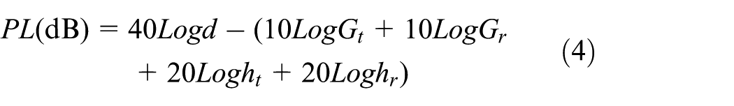
where h_t is the height of the transmitting antenna and h_r is the height of the receiving antenna. By equations (3) and (4), it can be seen that the energy consumption E has a power attenuation of four in relation to the distance.

Finally, the logarithmic attenuation model is suitable to work in both closed and open environments. In this model, it is assumed that the power signal decreases in a way that is inversely proportional to the square of the distance $1 / d_{ij}^{2}$ . In a real environment, you can assume that the signal can be affected by a factor $(1 / d_{ij})^{η_{ρ}}$ , where η_ρ is known as the attenuation factor and depends on geometric and environmental factors (such as reflection, diffraction, attenuation, and dispersion). Its practical value fluctuates between 2 and 4.¹⁸ The model can be represented by

P^{ij} = P_{0} (d_{0}) - 10 η_{ρ} Lo g_{10} (\frac{d_{ij}}{d_{0}}) + σ_{SH} = {\bar{P}}^{ij} + X_{σ}

(5)

where P^ij is the power received at the sensor s_j from the sensor s_i (measured in dBm). P₀(d₀) is a reference power at a distance d₀ transmitter (typically 1 km for large urban mobile systems and 1 m for indoor systems).¹⁹X_σ is a random variable, with Gaussian distribution that has an expected value of zero and a standard deviation σ_SH for cases of attenuation. Power measurements follow a logarithmic Gaussian distribution as shown below

P^{ij} ~ N ({\bar{P}}^{ij}, σ_{SH})

(6)

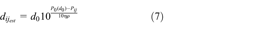
where P^ij is the expected value of the received power in dBm. From equations (5) and (1), the distance d_ij can be estimated as follows

d_{i j_{est}} = d_{0} 10^{\frac{P_{0} (d_{0}) - P_{ij}}{10 η ρ}}

(7)

DALSA

Consider a WSN deployed in a flat two-dimensional (2D), with a set of N anchor sensors A = {a₁, a₂, …, a_N}, where the sensors in the anchor set know their geographical position by GPS. The location of an anchor sensor is represented by the coordinates a_i = [a_xi,a_yi]^T, for i = 1, …, N. Commonly, N > 2 is used. In this research, we use N = 4 because only a small percentage of the sensors use GPS technology or another type of self-location.

Instead, a set M of unknown sensors U = {u₁, u₂, …, a_M} is deployed uniformly and randomly over the same area. Unknown sensors only have the technology to calculate the power of the received signal between neighboring sensors, it is considered a range R = 30 mts. It is considered a set of true positions from unknown sensors as u_j = [u_xj,u_yj]^T, for j = 1, …, M, and a set of estimated positions p_j = [p_xj, p_yj]^T. For purposes of the investigation, a value of M = 96 was used. Generally, the percentage of the anchor sensors with respect to unknown sensors is much higher, M ≫ N.

The algorithm is designed so that once the initial estimate of the position of a sensor s_i given by $p_{i}^{ι}$ , obtained in principle by Least Square, the sensor s_i produces a new position $p_{i}^{ι + 1}$ using only the positions and estimated distances with neighboring sensors

Ψ_{i} = {k ∣ ∥ u_{i} - u_{k} ∥ < R}

(8)

and reference sensors

Ω_{i} = {l ∣ ∥ u_{i} - u_{l} ∥}

(9)

and |Ψ_i|+|Ω_i| represent the cardinality of the set of neighboring sensors and anchors, respectively, of s_i.

The distributed algorithm determines for each unknown sensor s_i a search region called S_i. For each search region given, it is assigned a set of possible positions. S_i can vary in size according to the error distance with neighboring nodes. The idea is to limit the problem and divide it into sections, so that each sensor must estimate a position $p_{i}^{ι + 1}$ that could decrease the total error with its neighbor sensors. So that each sensor can gradually adapt to changes in neighboring sensors and thus eliminate the initial estimate error gradually.

The total error in the estimated position of each sensor can be defined as the sum of the errors between anchor sensors and unknown neighboring sensors. It is important to note that the anchor sensors in this research have connection to all sensors in the WSN; for purposes of the present investigation, the connection of the four anchor sensors with each unknown sensor is taken into account. Instead, unknown sensors have a range of 30 mts which is less than the anchor sensors reach.

To define the estimation error between the estimated position P _i of a sensor s_i and the estimated position P _j of a neighbor sensor s_j, the following expression is used

E_{i} = \sum_{j = 1}^{| Ψ_{i} | + | Ω_{i} |} | d_{ij} (p_{i}, p_{j}) - d_{i j_{est}} |

(10)

where d_ij(p_i,p_j) refers to the Euclidean distance between the sensor position s_i with respect to a neighboring sensor s_j

d_{ij} (p_{i}, p_{j}) = \sqrt{{(p_{x_{j}} - p_{x_{i}})}^{2} + {(p_{y_{j}} - p_{y_{i}})}^{2}}

(11)

Note that neighbor sensors s_j can be either an anchor or an unknown sensor. The sensor s_i coverage range delimits the exchange of information between the set Ψ_i and Ω_i. Therefore, the total error of s_i is calculated by performing the sum of the errors with respect to neighboring sensors including anchor sensors.

The total error in each sensor s_i is influenced to delimit the area of the search region for the new position $p_{i}^{ι + 1}$ . That is, in the search region S_i, n possible positions are uniformly and radially distributed and are allocated on the center point of the current position $p_{i}^{ι}$ of sensor s_i.

In Figure 1, the circular search region defined by a radius α with three levels can be observed. Where α is calculated by the following expression

α = \frac{E_{i}}{| Ω_{i} | + | Ψ_{i} |}

(12)

so, the length of the radius α changes with each iteration and will be different in each of the unknown sensors, since the error E_i is different for each individual case. With this we sought that at first the spacing would make the region out a wide search, which sought to reach the best error rate in a quick manner but with a robust search; however, as the iterations are advancing, the error decreases, so the spacing and the search region becomes thinner and more accurate.

Figure 1.

Circular search region for s_i with eight equally spatially distributed possible candidates in each orbit.

For the search region S_i of each sensor s_i, a number n = 25 of possible positions is assigned. It is important to note that the spacing between levels of search was α, and it has divided in three levels of searching.

To determine its new position, the sensor s_i evaluates each candidate position of S_i into the equation (10). Thus, the position that minimizes this equation becomes $p_{i}^{ι}$ , where $p_{i}^{ι}$ will be used by neighboring sensors of s_i to recalculate their new positions and so on. Therefore, the algorithm can run until the user applies a stop flag or put a threshold value.

Simulation results

It was decided to implement a bank of WSNs through simulation under two schemes, C-shape and uniform-randomly distributed, to perform the corresponding tests on the DALSA algorithm and the other algorithms to be tested. The simulation was carried out on MATLAB. We made a total of 20 simulated WSNs for each scheme, so the test of each algorithm was made on each one at time.

For each scheme, in a 2D area, we randomly deployed a total of 100 sensors nodes in a square area of 100 m × 100 m, where 96 of those sensors are considered as unknown sensors and four of them are anchors sensors which know their own position. On the other hand, the estimated distance d_ijest between neighboring sensors was simulated under two approaches. The first approach consists of adding a noise component that has a Gaussian distribution where d_ijest is calculated by the following expression

d_{i j_{est}} = \sqrt{{(x_{jt} - x_{it})}^{2} + {(y_{jt} - y_{it})}^{2}} \times noise

(13)

Where the noise can be described as

noise = \max [0, 1 + E_{ij} \times n f_{d}]

(14)

And E_ij is a normal random variable N(0,1) representing the measurement noise. Then, nf_d is the noise factor (standard deviation of the distance error in percentage) for the distance measurements.²⁰ For a standard deviation of 20% in the distance estimation error, we set nf_d = 0.20.

The second approach used to estimate distance between neighboring sensors was the RSS methodology described in section “Distance estimator” with σ_SH = 2 and η_p = 2.6 which correspond to indoor environments.¹⁹

For the algorithm evaluation, three algorithms found in the recent state of the art were used as reference. The first algorithm against was compared with the DSCL,²¹ the second algorithm was the Levenberg Marquardt,^22,23 and the third one was the SOCP^15,16 algorithm. The main characteristics evaluated were the estimation accuracy and the iterations to converge. A set of initial positions were produced using least squares only with the location information produced by anchor nodes. As described earlier, we assume that the four anchors have connectivity with all unknown sensors, each algorithm was ran for 100 iterations in each one of the 20 simulated networks and the accuracy was measured using the root mean square error (RMSE)

RMSE = \sqrt{\frac{1}{N} \sum_{j = 1}^{N} {| | p_{i}^{ι} - u_{i} | |}^{2}}

(15)

where N is the number of unknown sensors in each network, and $| | p_{i}^{ι} - u_{i} | |$ is the Euclidean distance between the last position estimated p_i and the true position u_i for a sensor s_i.

Figure 2 shows an example of a uniform and randomly distributed WSN with the last estimated positions using DALSA versus the real positions of the unknown sensors using a nf_d = 0.10 resulting in an average error of 2.24 m. An initial estimation was made using the least square technique, so the initial error on this example was 18.2 m. Also there was not a threshold applied to stop the iterations, so it ran for 100 iterations but the RMSE reaches the lowest value after 15 iterations.

Figure 2.

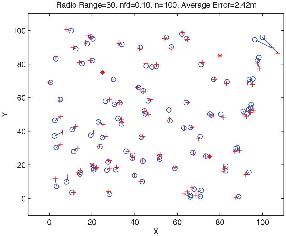
Position estimates of DALSA using a network with 96 unknown sensors with nf_d = 0.1 and initial estimates provided by the least square method.

Figure 3 shows an example of a C-shape distributed WSN with the last estimated positions using DALSA versus the real positions of the unknowns sensors using a nf_d = 0.10.

Figure 3.

Position estimates of DALSA using a network with 96 unknown sensors with nf_d = 0.1 and initial estimates provided by the least square method in a C-shape distribution.

Figure 4 shows a comparison of RMSE values after 100 iterations for different algorithms using a nfd = 0.20 with a random and uniform deployment topology. The RMSE follows a negative exponential behavior in almost every case. The DSCL and DALSA algorithms present a fast decay at almost five iterations, but DALSA shows the minimum error rate in the long term.

Figure 4.

RMSE behavior of the proposed DALSA algorithm with nf_d = 0.20 and uniform topology versus other algorithms.

Table 1 shows the average RMSE of 20 WSN with a standard deviation of 20%. The Δ symbol means the threshold used as a reference for the change in the RMSE value, and it can be represented as follows

| RMS E^{ι} - RMS E^{ι + 1} | \leq Δ

(16)

Table 1.

20 WSNs average, uniform and random deployment with R = 30 m, initial RMSE estimate = 23.33 m.

nf_d = 0.20, Δ = 0.1
Algorithm	Iterations	RMSE (m)
DALSA	6	3.3442
LM	8	7.1621
DSCL	6	3.6306
SOCP	3	10.6447

WSN: wireless sensor network; RMSE: root mean square error; DALSA: distributed adaptive local searching algorithm; SOCP: second-order cone programming.

As shown in Table 1, the SOCP algorithm is the fastest to achieve a minimum change of Δ followed by the LM algorithm, but the most accurate algorithms are the DSCL and the DALSA, with DALSA achieving almost half of the RMSE recorded by LM.

The second test made was with a nf_d = 0.20, but now with a C-shape distribution as shown in Table 2. The initial RMSE was 26.9065 m which implies an increment of almost 3 m compared to the average RMSE of the WSNs with a uniform and random distribution. The lowest RMSE was accomplished by the DALSA algorithm with a magnitude of 4.8024 m as depicted in Figure 5.

Table 2.

20 WSNs average, regular deployment in C-Shape area with R = 30 m, initial RMSE estimate = 26.9065 m.

nf_d = 0.20, Δ = 0.1
Algorithm	Iterations	RMSE (m)
DALSA	8	4.8024
LM	8	7.7798
DSCL	8	5.5431
SOCP	2	8.9595

WSN: wireless sensor network; RMSE: root mean square error; DALSA: distributed adaptive local searching algorithm; SOCP: second-order cone programming.

Figure 5.

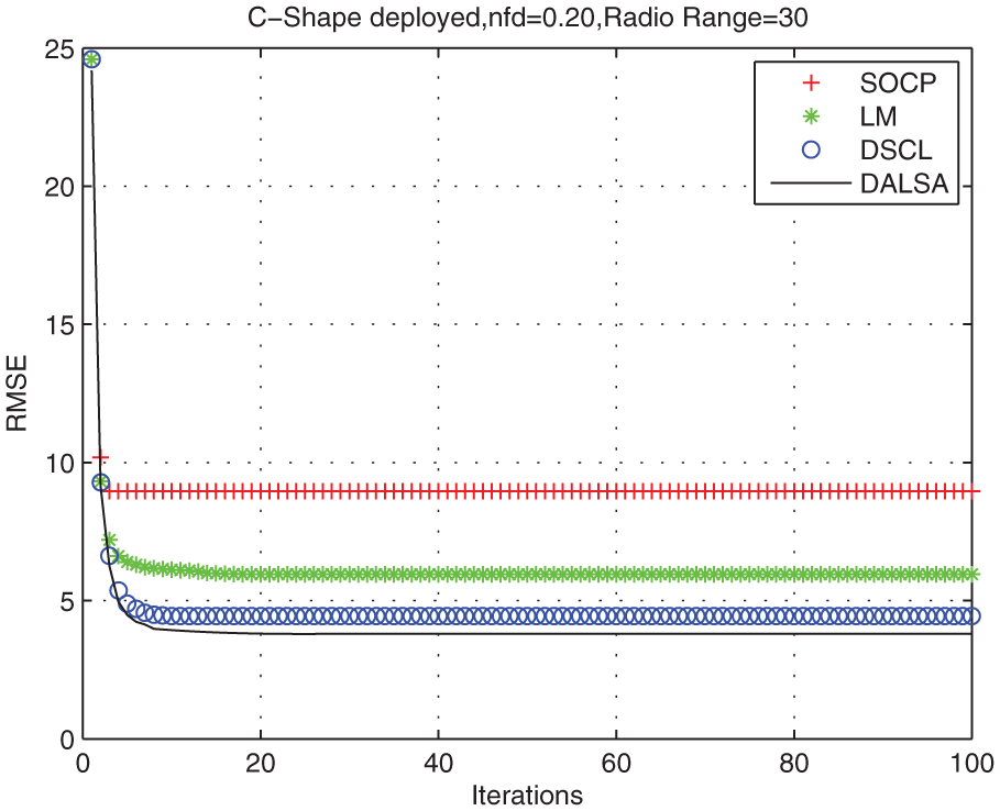
Proposed DALSA algorithm with nf_d = 0.20 and C-shape distribution versus other algorithms.

Again, SOCP algorithm was the fastest to accomplish the minimum threshold, but the RMSE has a really poor accuracy compared to the other three algorithms. In this case, there was only 0.7 m of difference on the RMSE when Δ was lower than 0.1. DALSA algorithm accomplished the lowest RMSE.

We also run a test with the RSS model. The RSS was used with a uniform and randomly distribution as well in a C-shape one. We used least squares to estimate initial positions. Figure 6 shows the RMSE behavior of the four algorithms, the initial RMSE for each one was 20.43 m. The average RMSE was almost identical on the DSCL and the DALSA algorithms, but DALSA algorithm obtained a lower RMSE average of 4.4802 m.

Figure 6.

RMSE behavior of the proposed DALSA algorithm with RSS in a uniform and random deployment versus other algorithms.

As shown in Table 3, the slowest algorithm to converge is the LM, at the nine iteration. The DALSA algorithm reaches the best accuracy at six iterations.

Table 3.

20 WSN average, uniform and random deployed, R = 30, initial RMSE estimate = 20.43.

RSS, Δ = 0.1
Algorithm	Iterations	RMSE (m)
DALSA	6	4.4802
LM	9	6.1928
DSCL	8	4.8536
SOCP	2	7.9171

WSN: wireless sensor network; RMSE: root mean square error; RSS: received signal strength; DALSA: distributed adaptive local searching algorithm; SOCP: second-order cone programming.

The RSS model was also used in a C-shape distribution. Figure 7 shows the RMSE behavior and the results obtained after 100 iterations. It can be seen that DALSA algorithm presents the best results in accuracy and also in convergence speed.

Figure 7.

RMSE behavior of the proposed DALSA algorithm with RSS in a C-shape deployment versus other algorithms.

Table 4 shows a summary of the tests realized under the two approaches proposed to estimate distances between neighboring sensors, as well as the two topologies used.

Table 4.

Summary results using different topologies.

Sensor deployment	Distance estimation	RMSE initial estimates	RMSE final estimates
Sensor deployment	Distance estimation	RMSE initial estimates	SOCP	LM	DSCL	DALSA
C-shape	nf_d = 0.10	11.4918	7.7165	2.2794	2.2756	2.1292
	nf_d = 0.15	17.2047	10.5596	4.3942	3.8588	2.9453
	nf_d = 0.20	26.9065	8.9595	7.7798	5.543	4.8024
	RSS	20.2451	9.6098	5.5658	4.598	4.2529
Uniform and random	nf_d = 0.10	11.3876	6.2811	1.7739	1.9389	1.6926
	nf_d = 0.15	18.2014	8.8385	3.4249	2.5948	3.6141
	nf_d = 0.20	23.3336	10.6447	7.1621	3.6306	3.3442
	RSS	20.4381	7.9171	6.1928	4.8536	4.4802

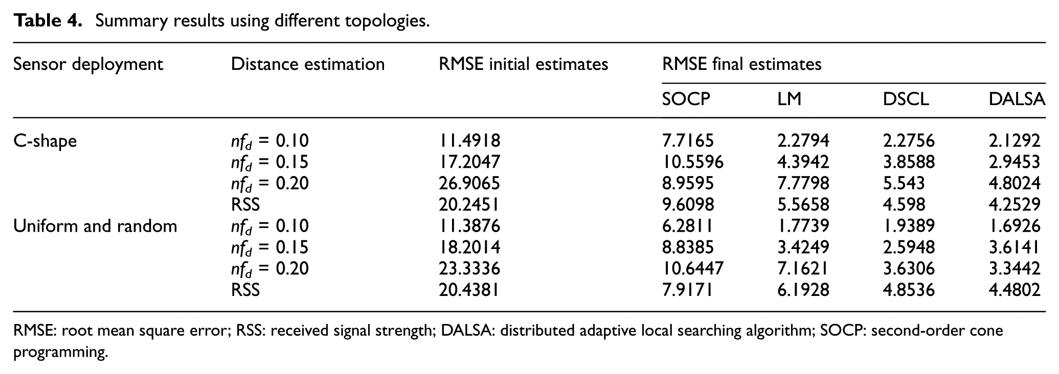
RMSE: root mean square error; RSS: received signal strength; DALSA: distributed adaptive local searching algorithm; SOCP: second-order cone programming.

Finally, we proposed to make a test using the same scenario provided by¹⁶ the total number of sensors n = 300, the sensors were randomly deployed on a [−0.5,0.5]² area. The percentage of anchor sensors was 40%. Also, there was used a nf_d = 0.05. The main difference in this approach was the nonuse of an initial estimator, all of the unknown sensor positions were initiated at [0,0]. The RMSE results can be seen on Figure 8.

Figure 8.

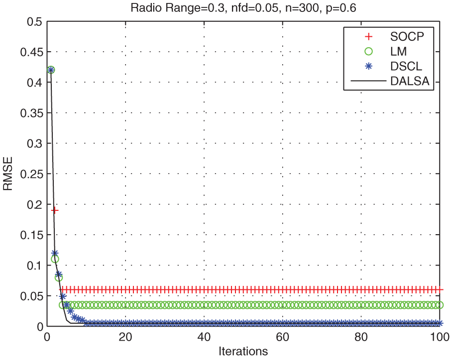
RMSE behavior of the proposed DALSA algorithm and others without using an initial estimator.

The results were practically the same using the DSCL and DALSA algorithms, they showed the most accurate RMSE, but DALSA showed the fastest converge time, as it is shown the DALSA algorithm converges at almost fourth iteration while DSCL converges at eighth.

Conclusion and future work

This article proposes a novel DALSA for range-based localization in WSNs. The main purpose of the algorithm was to reduce the high error in estimated positions caused by the noisy estimated distances between the sensors in a WSN. The method is a decentralized and iterative algorithm.

Our algorithm was compared to other three algorithms found in the recent state of art. The simulation results confirm the superiority of our proposed algorithm in terms of estimation accuracy and convergence. Unlike other existing algorithms, our approach has a good response when the percentage of anchor nodes is reduced.

The proposed approach could have better results in terms of accuracy if the set possible positions for the adaptive region increases, but that could decimate the computer efficiency. That is why the number of positions was set on 25. Also, the algorithm shows that it requires few iterations to converge, not as fast as SOCP, but has a much better accuracy than it.

As future work, we would like to evaluate the time of processing of each node and compare it to other algorithms. Finally, we are also interested in evaluating our algorithm in a real WSN.

Footnotes

Academic Editor: Yong Feng

Declaration of conflicting interests

The author(s) declared no potential conflicts of interest with respect to the research, authorship, and/or publication of this article.

Funding

The author(s) disclosed receipt of the following financial support for the research, authorship, and/or publication of this article: This work was supported by the National Council for Science and Technology (CONACyT), Mexico.

References

Shen

Wang

Jiang

. Connectivity and RSSI based localization scheme for wireless sensor networks. In: Huang

D-S

Zhang

X-P

Huang

G-B

(eds) Advances in intelligent computing (Lecture notes in computer science), vol. 3645. Berlin, Heidelberg: Springer, 2011, pp.578–587.

Tang

Qian

A centralized location algorithm based on RSSI in large-scale wireless sensor network. Proced Eng 2011; 15: 2004–2009.

Zhang

Yang

An enhanced DV-Hop localization algorithm using RSSI. Int J Future Gener Commun Netw 2013; 6(6): 91–98.

Salman

Ghogho

Kemp

Optimized low complexity sensor node positioning in wireless sensor networks. IEEE Sens J 2014; 14: 39–46.

Livinsa

Jayashri

An ingenious localization algorithm for WSNs with and without obstacles. IUP J Telecommun 2014; 6(2): 42–53.

Huang

Zheng

Xio

Robust localization algorithm based on the RSSI ranging scope. Int J Distrib Sens N 2015; 2015: 1–8.

Safa

A novel localization algorithm for large scale wireless sensor networks. Comput Commun 2014; 45: 32–46.

Wang

Wan

Liu

A novel ranging method based on RSSI. Energy Proced 2011; 12: 230–235. (also published in the proceedings of international conference on smart grid and clean energy technologies (ICSGCE 2011)).

Shu

Yan

Liu

L-I.

Improved three-dimensional localization algorithm based on volume-test scan for wireless sensor networks. J China Univ Posts Telecommun 2012; 19(Suppl. 2): 1–6.

10.

Rahman

Park

Kim

K-D.

RSS-based indoor localization algorithm for wireless sensor network using generalized regression neural network. Arab J Sci Eng 2012; 37(4): 1043–1053.

11.

Hou

Huang

A framework based on barycentric coordinates for localization in wireless sensor networks. Comput Netw 2013; 57(17): 3701–3712.

12.

Meng

Xie

Xiao

Decentralized TDOA sensor pairing in multihop wireless sensor networks. IEEE Signal Proc Let 2013; 20: 181–184.

13.

Jama

Kouba

Kayani

EasyLoc: RSS-based localization made easy. Proced Comput Sci 2012; 10: 1127–1133.

14.

Jiang

Zheng

Chen

. A distributed RSS-based localization using a dynamic circle expanding mechanism. IEEE Sens J 2013; 13: 3754–3766.

15.

Tomic

Beko

Dinis

Distributed RSS-based localization in wireless sensor networks based on second-order cone programming. Sensors 2014; 14(10): 18410.

16.

Tomic

Beko

Dinis

. Distributed RSS-based localization in wireless sensor networks using convex relaxation. In: International conference on computing, networking and communications (ICNC), Honolulu, HI, 3–6 February 2014, pp.853–857. New York: IEEE.

17.

Svecko

Malajner

Gleich

Distance estimation using RSSI and particle filter. ISA T 2015; 55: 275–285.

18.

Patwari

Ash

Kyperountas

. Locating the nodes: cooperative localization in wireless sensor networks. IEEE Signal Proc Mag 2005; 22: 54–69.

19.

Andersen

Rappaport

Yoshida

Propagation measurements and models for wireless communications channels. IEEE Commun Mag 1995; 33: 42–49.

20.

Srirangarajan

Tewfik

Luo

ZQ.

Distributed sensor network localization using SOCP relaxation. IEEE T Wirel Commun 2008; 7: 4886–4895.

21.

Cota-Ruiz

Rosiles

J-G

Rivas-Perea

. A distributed localization algorithm for wireless sensor networks based on the solutions of spatially-constrained local problems. IEEE Sens J 2013; 13: 2181–2191.

22.

Cota-Ruiz

Rosiles

J-G

Sifuentes

. A low-complexity geometric bilateration method for localization in wireless sensor networks and its comparison with least-squares methods. Sensors 2012; 12(1): 839.

23.

Dennis

Jr Schnabel

RB.

Chapter 10. Nonlinear least squares. In: Dennis

Jr Schnabel

RB.

(eds) Numerical methods for unconstrained optimization and nonlinear equations. Upper Saddle River, NJ: Prentice Hall, 1983, pp.218–238.

A distributed adaptive local searching algorithm for wireless sensor network localization

Abstract

Keywords

Introduction

Related work

Distance estimator

DALSA

Simulation results

Conclusion and future work

Footnotes

Declaration of conflicting interests

Funding

References