
Abstract
The article addresses the modeling and performance analysis of wireless sensor network localization with direct-sequence spread-spectrum signals and network-based, time difference of arrival measurements. Realistic radio channel propagation and interference conditions are taken into account. Synchronization by means of a delay-locked loop is adopted for sensor signal tracking at the wireless sensor network anchor nodes. A comprehensive timing estimation analysis is presented with channel impairments, including pathloss attenuation, shadowing, multipath fading, and multi-access interference. The full statistics of the delay-locked loop tracking jitter are derived, which serves to assess the practically achievable synchronization accuracy and its variability with radio channel conditions and specific sensor location. The time difference of arrival measurements are then used for sensor localization based on an efficient iterative maximum likelihood estimation approach shown to outperform weighted least squares methods. Numerical results are presented to quantify the sensor localization accuracy limits, showing that the error is not uniform but varies considerably across the coverage region depending on the relative sensor position with respect to the different anchor nodes. Various factors related to changing wireless sensor network topologies and network loading conditions are also considered and their impact on localization performance is quantified.
Keywords
Introduction
Wireless sensor networks (WSNs) have several advantages and are recently finding widespread use and many applications in various fields.1–3 One of the features of WSNs is the ability to support node localization and tracking with good accuracy, and several WSN localization techniques have received a lot of interest in the literature (see, for example, the works of Kulaib et al., 4 Boukerche et al., 5 and Mao et al., 6 and references therein). In general, network-based localization can be achieved by means of statistical signal processing algorithms that exploit time of arrival (TOA), time difference of arrival (TDOA), angle of arrival (AOA), and received signal strength (RSS) measurements from transmitted sensor node (SN) signals collected at a number of fixed anchor nodes (ANs). 7 Other terminal-based localization techniques rely on processing signals at the mobile SNs but are of less interest in WSN deployments since low-cost, limited-power SNs cannot implement intensive processing algorithms. Recent WSN localization applications have thus mainly focused on network-based AN processing. A review of previous related techniques is presented in the next section. In particular, timing-based approaches, combined with broadband spread-spectrum signaling waveforms, can support reliable target positioning due to their high timing resolution and resistance to noise and interference. TDOA schemes, which use the differences of sensor signal epochs of arrival at the receiving ANs, do not require perfect timing alignment of SNs with the network infrastructure and have less stringent synchronization requirements, which make them amenable to low-complexity WSN implementations. As such, the present work focuses on TDOA-based localization and analyzes the achievable localization accuracy in realistic WSN propagation environments. 8 More specifically, among the important challenges not previously addressed is the large variation in SN signal hearability at the multiple network nodes needed for TDOA localization (which requires at least four AN timing measurements). The SN signal may not be adequately received at remote ANs, especially under severe pathloss and shadowing conditions as well as interference from other active transmitters. It is therefore important to analyze these aspects and assess their impact on localization performance.
Accordingly, a first contribution of this work presents a detailed analysis of signal timing of arrival estimation by means of a delay-locked loop (DLL) under applicable radio propagation and multi-user interference. The use of the DLL is crucial for fine tracking of signal timing, 9 and its performance is shown to be strongly dependent upon RSS and multipath fading conditions. The specific error statistics are obtained at each AN involved in sensor positioning. The analysis shows that the accuracy of timing estimation is highly sensitive to the radio propagation environment and SN relative position vis-à-vis different ANs, which provides important insights into the limits of timing measurements under realistic operating conditions. In a second contribution of the work, the obtained DLL tracking results are combined with an efficient iterative maximum likelihood algorithm 10 and adapted for TDOA localization. The viability of the proposed method is demonstrated with numerous examples for different sensor and AN locations and network loading conditions, and benchmarked against other methods and theoretical bounds. 11
The rest of the article is organized as follows. First, a review of previous work is presented in the “Related work” section. The system and signal models are then introduced in the “System and signal models” section. The “Signal timing estimation” section presents the analysis of DLL time tracking and derivation of its error statistics. In the “TDOA localization performance analysis” section, the maximum likelihood TDOA localization algorithm is presented, and numerical results and discussions are given in the “Results and analysis” section, with final conclusions summarized in the “Conclusion” section.
Related work
Different approaches, such as those presented in the literature,12–16 use RSS-based data that exploit readily available signal strength measurements. Filtering and combined differential localization is adopted in Adewumi et al. 17 to further smooth RSS data, while adaptive processing to enhance performance is proposed in Chen et al. 18 and Zhang et al. 19 However, the RSS-based approaches are generally vulnerable to large dynamic range and severe shadowing, and fading conditions encountered in radio channels. 20 On the other hand, AOA-based techniques require complex antenna arrays and are not practical to use in low-cost, reduced-complexity deployments. 7 A different perspective for radiation source detection using a network of detectors is introduced in Chase et al.’s study, 21 which proposes a source-attractor radiation detection approach. In another aspect, timing-based techniques including TOA and TDOA are more commonly used for WSN localization due to their robustness. A survey of TOA methods is presented in Guvenc and Chong 22 and Xu et al., 23 and in Yu et al. 24 and Mekonnen and Wittneben, 25 clock frequency offsets and node position uncertainties are taken into consideration. However, it is noted that TOA-based techniques need to have precise knowledge of SN transmission epochs, and maintain strict timing alignment of the sensors with the WSN reference clock, which adds more constraints to the synchronization complexity of the SNs and WSN infrastructure. To the contrary, TDOA localization schemes do not require knowledge of the sensors’ exact transmission times as long as the ANs have a common timing reference. TDOA-based approaches were introduced in Bandiera et al. 26 and Wang et al. 27 based on iterative and constrained least squares algorithms. In Luo et al., 28 a geometric-based approach for successively localizing neighboring sensors is proposed, and asynchronous WSNs are considered in Xiong et al. 29 based on a simplified linearization model used with maximum likelihood estimation. Distributed sensor localization using TDOA with frequency-hopping signals is analyzed in Zhang et al., 30 and a different approach based on neural networks is proposed in Singh and Agrawal, 31 while Ghelichi et al. 32 introduce another geometric TDOA localization technique. However, it is noted that these works adopt simplistic timing error models and hypothetical assumptions in the positioning algorithms without considering the impact of actual timing estimation limitations and large discrepancies among different ANs in tracking the targeted SN signal under realistic channel impairments and increased interference conditions, which motivates the studies undertaken in this present work.
System and signal models
A WSN model is considered with a central AN serving the SNs of interest, surrounded by a number of additional nodes as shown in the layout of Figure 1.
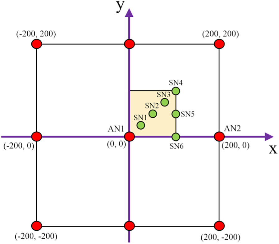
WSN with selected sensor node (SN) and anchor node (AN) placement.
The transmitted signal from a given SN is assumed to undergo small-scale fading and large-scale attenuation due to radio pathloss and shadowing. For large-scale attenuation, we use typical models, which include both deterministic and probabilistic components. More specifically, based on the experimental results of Martinez-Sala et al.,
8
we adopt a two-slope pathloss propagation model with random shadowing effects, whereby the SN signal attenuation (in dB) at distance

where

where

with
For the modulation scheme, the transmitted signal from a given SN is assumed to use direct-sequence spread-spectrum (DS-SS) waveforms with binary phase shift keying (BPSK), 33 the signal at a given anchor node AN i involved in sensor localization, may be expressed as

where
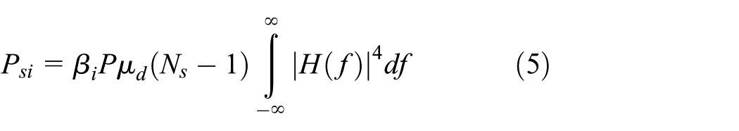
where

where
In the subsequent numerical results, the relative average power factors and other-cell interference will be obtained by simulation of the radio propagation model with its pathloss attenuation and shadowing assumptions, and will have a noticeable impact on the accuracy of sensor signal timing estimation at different ANs.
Signal timing estimation
DLL timing synchronization
The accuracy of sensor position determination is highly dependent upon the performance of TOA estimation. For the DS-SS signaling schemes used in this work, accurate synchronization tracking is typically achieved by means of a DLL mechanism that follows coarse timing acquisition.
9
A non-coherent DLL structure, as depicted in Figure 2, is used to avoid coherent carrier synchronization and data demodulation prior to de-spreading. The targeted sensor served by the central anchor station AN1 must also be tracked by other ANs as well (four nodes are needed for TDOA localization). For each anchor node AN
i
involved in the sensor positioning, a DLL device is used to track the timing of the received sensor signal. The relative delay

Delay-locked loop processing blocks.
For the DLL operation, the received signal is first mixed with a local oscillator (LO) for down conversion, and then fed to early and late branches having timing offsets of

where
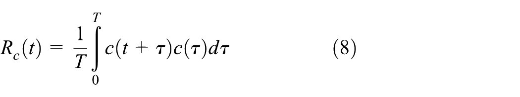
Using a discrete-time sampled structure, the kth sample normalized tracking error is defined by

The discretized loop discriminator output becomes

where

with an early–late loop offset
The statistics of the timing error estimates are of primary interest in the performance analysis of positioning algorithms. This is considered next under the general model assumptions of the “System and signal models” section.
Time tracking statistics analysis
A digital DLL model is adopted in this work, and the timing estimates are recursively given by

where

For a simple first-order filter

The recursive SDE obeys a first-order Markov random process, where the Nakagami-m random sample
where

with parameters

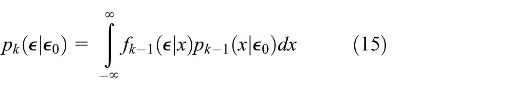
From equation (14), the random variable

Defining the random variables

Using conditional independence of the variables Z and V, the transition PDF is obtained by convolving the conditional PDFs, giving

The DLL error statistics can thus be obtained and will be applied for various cases of interest in the localization examples discussed in the “Results and analysis” section.
Evaluation of timing estimation accuracy
To quantify the signal timing estimation performance, numerical results for the DLL tracking are presented. For the signaling waveforms, a root raised cosine waveform spectrum with 25% roll-off, a 256 spreading factor, and a chip period of 5 ns are assumed. As noted, propagation models applicable to outdoor WSN environments are taken into account to assess the performance variability as a result of changing SN location vis-à-vis different ANs in the WSN.
To take into consideration interference from other sensors served by multiple ANs, a WSN network is assumed with 25 ANs placed on a rectangular grid with 200 m maximum AN-AN separation, corresponding to an SN-to-AN range within a 100 m, as a realistically achievable coverage limit. The WSN layout provides two tiers of ANs surrounding the central AN1 of interest, which is adequate to accurately model the interference environment. The other-cell interference factor was obtained by Monte Carlo simulation used to generate sensors uniformly spread across the WSN coverage area, where each sensor’s transmitted power is adjusted to yield a specific received power at their dedicated serving AN. The interference power from all sensors not belonging to the AN1 coverage zone is then aggregated and divided by the interference accrued from other sensors served by the central AN1, besides the sensor of interest. This yields the relative other-cell to same-cell interference ratio koc of equation (6). The simulations show that this factor is particularly sensitive to the pathloss exponents of the radio attenuation model, as seen from the numerical results shown in Table 1. The random shadowing was also found to increase the
Relative other-cell interference factor

To assess the impact of the sensor power levels at various access nodes, selected sensor locations are chosen at different points throughout the coverage area. Referring to Figure 1, representative sensors are denoted as SN1 through SN6, with coordinates (25,25), (50,50), (75,75), (100,100), (50,0), and (100,0), respectively. Other choices are also possible, but the main purpose is to investigate the variability in power levels and the proximity to one, two, or all four ANs needed for TDOA sensor localization. By symmetry, other choices from different sub-triangles will give similar results. In addition, the average performance for uniformly distributed sensors in the coverage zone will be assessed in the next section. Referring to the average power levels received at the access nodes, Table 2 shows the βi power factors for different SN points. Without loss of generalization, the
Average power factors at different ANs for sensors SN1 through SN6.

SN: sensor node; AN: anchor node.
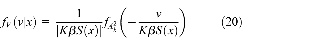
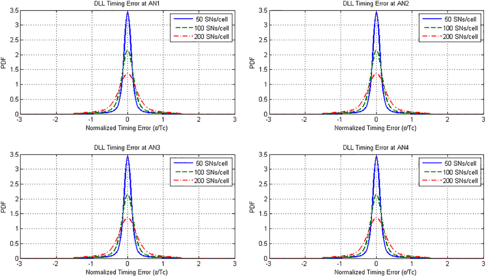
Table 3 summarizes results for the DLL tracking at AN1 to AN4, and it is seen that the change in timing estimation jitter (quantified by the timing standard deviation) among the selected SN positions for each of the ANs is indeed consistent with the previous observations, whereby higher jitter is observed at the more distant ANs from the SNs of interest. For the results of Table 3, a uniform loading of 50 sensors per coverage cell across the WSN was assumed, with a data activity factor set to 10% as noted previously. To gain further insight into the impact of increased sensor loading, we consider two other levels, namely, 100 and 200 sensors per cell. The corresponding DLL timing error PDFs are obtained using the analysis of the “Signal timing estimation” section, and the results are plotted in Figures 3–8. The impact of increased cell loading resulting in wider-spread DLL error PDFs is clearly seen. Also, the sensors’ relative proximity to ANs affects their timing tracking. For instance, SN1 timing estimation at AN1 is very good but is much poorer at the other ANs. On the other hand, SN4 is equally well tracked by all nodes, while SN6 is better tracked at AN1 and AN2. It should be noted that the DLL tracking ranges have been limited to ±1.5Tc as errors beyond this range are assumed to lead to out-of-lock condition, triggering new timing acquisition. In summary, the obtained results serve to quantify the large differences in timing synchronization capabilities for WSNs with different radio channel conditions, loading levels, and deployment topology.
DLL timing SD at the four ANs receiving sensor signals.

DLL: delay-locked loop; SD: standard deviation; AN: anchor node; SN: sensor node.
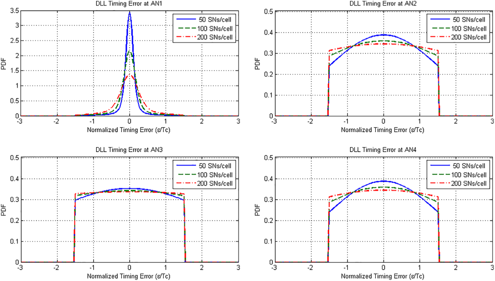
DLL tracking error PDFs at access nodes AN1 to AN4 for sensor SN1 (25,25), with various cell loading and interference conditions: 50, 100, and 200 sensors per cell.

DLL tracking error PDFs at access nodes AN1 to AN4 for sensor SN2 (50,50), with various cell loading and interference conditions: 50, 100, and 200 sensors per cell.

DLL tracking error PDFs at access nodes AN1 to AN4 for sensor SN3 (75,75), with various cell loading and interference conditions: 50, 100 and 200 sensors per cell.
DLL tracking error PDFs at access nodes AN1 to AN4 for sensor SN4 (100,100), with various cell loading and interference conditions: 50, 100, and 200 sensors per cell.

DLL tracking error PDFs at access nodes AN1 to AN4 for sensor SN5 (100,50), with various cell loading and interference conditions: 50, 100, and 200 sensors per cell.
DLL tracking error PDFs at access nodes AN1 to AN4 for sensor SN6 (100,0), with various cell loading and interference conditions: 50, 100, and 200 sensors per cell.
TDOA localization performance analysis
Iterative maximum likelihood TDOA algorithm
As noted, TDOA-based localization is well suited for WSNs, where low-complexity, power-limited SNs may not be able to maintain tight synchronization with the WSN. In this work, we use an iterative approximate maximum likelihood (AML) localization technique introduced in Chan et al. 10 However, rather than assuming hypothetical and unrealistically identical timing error statistics at different ANs, the DLL analysis is used with the signal attenuation and fading models, interference loading conditions, and sensor placement variations, discussed in the “Signal timing estimation” section, to obtain the specific timing error variances.
With regard to TDOA localization, it is known that the differences in times of arrival of the sensor signal at a minimum of four access nodes are needed (with AN1 taken as reference node). Referring to Figure 1, the exact range between the ith AN and the sensor to be localized is

where

With noisy measurements, the variables

where c is the speed of light, and the variable

For compact notation, the following vector variables will be used subsequently


It is also noted that the TDOA measurements are correlated since they have a common term t1. Therefore, the covariance matrix

where

where
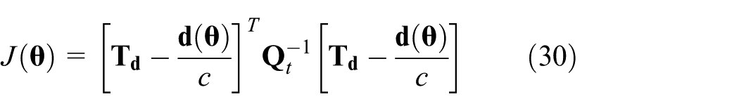
The maximum likelihood estimator (MLE) of the position vector

where


It then follows that

with

where


It is noted that, although the formulation in equations (35) to (38) gives a linear equation in the unknown position vector
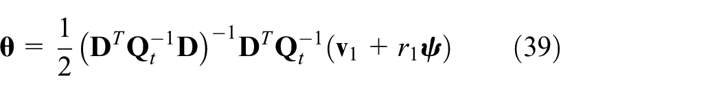
This gives

The resulting solution is obtained in terms of
Cramér–Rao lower bound analysis
The Cramér–Rao lower bound (CRLB) is a known fundamental limit in estimation theory that gives a lower bound on the minimum achievable variance of unbiased estimator.
11
The CRLB provides a benchmark for assessing the optimality of estimation techniques and is obtained from the Fisher Information Matrix (FIM), which depends on the PDF of the measurements, parameterized by the sensor position

where

From equation (23), we readily have
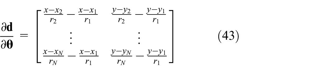
with the covariance matrix of the

The CRLB can be used to assess the efficiency of the TDOA AML algorithm by comparing it with the residual mean squared error (MSE) of the estimated sensor coordinates, as presented next.
Results and analysis
Numerical results are presented to evaluate the WSN sensor positioning accuracy and its dependency on various factors of interest. First, in Figure 9, we illustrate the residual localization error cumulative distribution functions (CDFs) giving Prob.[error <= abscissa] achieved by applying the TDOA AML. The CDFs are shown for the representative sensor locations SN1 through SN6, and the results confirm the previous observations and clearly demonstrate that positioning is more accurate for centrally located sensors at comparable distance from all ANs, while the accuracy worsens as they move further away from the center. Better accuracy is also noticed for sensors closer to two ANs (e.g. SN5 and SN6). Table 4 further shows quantitative results for the error percentiles giving thresholds that upper-bound the location error with a given probability. For example, the 50th percentile (which also corresponds to the mean error, as the CDFs are practically Gaussian-distributed) gives a mean value 0.25 m for SN4 followed by 0.34 and 0.41 m for SN5 and SN3, respectively, while it is 0.91 m for SN1. Similar observations hold with the 67th and 90th percentiles as well. For example, the 90% percentile giving the value below which the position error is confined with probability 0.9 (indicative of poor performance figure) is seen to be ranging from 0.46 m for SN4 to 1.91 m for SN1.

Comparison of localization error cumulative distribution functions for selected SN locations.
Examples of residual positioning error percentiles for SNs—SN1 through SN6.

SN: sensor node.
A comparative assessment of the adopted AML localization algorithm with another commonly used approach based on WLS estimation is also shown in Figure 10 which depicts the CDFs of the residual localization error for several SNs. The comparisons clearly show that the proposed AML offers improved accuracy over the WLS method. In another aspect, to illustrate the variability in localization accuracy across the WSN, the iterative AML average performance is depicted by the color plot in Figure 11, which shows contours of equal residual MSE as a function of sensor coordinates in the coverage zone. It is noted that the MSE is lowest when the sensor is close to the center (at comparable distance from all ANs), while it is highest as it gets close to its home AN. To further demonstrate the viability of the proposed TDOA MLE localization technique, a similar color plot is given in Figure 12 based on the CRLB bound, and it can be seen that the CRLB results are in line with the previous observations, which validates the efficiency of the iterative MLE algorithm used in this work.

Performance comparison of the proposed AML and WLS approaches.

TDOA AML algorithm mean squared error (MSE) dependence on sensor coordinates.

TDOA CRLB minimum achievable bound and its dependence on sensor coordinates.
In addition to the previous results obtained with a network loading of 50 sensors per cell, we illustrate in Figure 13 the impact of increased loading by considering 100 and 200 sensors per cell. The results show CDFs for the localization error assuming the sensors are uniformly distributed across the coverage zone. As expected, higher loading causes a deterioration in localization accuracy due to higher interference and subsequent increase in DLL timing jitter. As an example, the results of 50th percentile (mean) error are 0.54, 0.66, and 0.81 m for 50, 100, and 200 sensors per cell, respectively. Finally, in Figure 14, we investigate the impact of increasing the number of access nodes involved in TDOA sensor positioning (beyond the minimum number of four), and it can be seen that some incremental improvements in accuracy are achieved by using five and six ANs, especially if we consider the higher error percentile ranges (around 90%). However, it should also be noted that these small improvements are at the expense of increased messaging and processing complexity.

Cumulative distribution functions (CDFs) for the average localization error across the coverage area. Comparison of different cell loadings: 50, 100, and 200 sensors per cell.
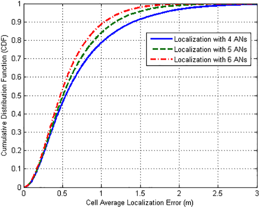
Cumulative distribution functions (CDFs) for the average localization error across the WSN coverage area. Comparison for the results of TDOA localization using four, five, and six anchor nodes.
Conclusion
The article dealt with the performance analysis of TDOA positioning in WSNs employing DS-SS signals. A detailed radio propagation model incorporating pathloss, shadowing, and fading effects was used to assess the realistic capability of DLL time tracking of the sensors’ emitted signals at the ANs involved in positioning. The effect of MAI was also taken into account. It was found that the large variability in received power levels at different ANs has a major impact on synchronization accuracy depending on the sensor’s relative position with respect to the different ANs. Using the DLL tracking statistics, an iterative maximum likelihood technique was adopted for TDOA positioning, and validated by comparison with other approaches and theoretical bounds. It was found that the localization performance varies considerably across the coverage zone, whereby accuracy is best for sensors located in the central part at comparable distance from all access nodes, while the error deteriorates as the sensor gets closer to its main serving AN. Several simulations and numerical results were presented to quantify the achievable sensor localization accuracy under different radio channel impairments and network operating conditions.
Footnotes
Handling Editor: Chase Wu
Declaration of conflicting interests
The author(s) declared no potential conflicts of interest with respect to the research, authorship, and/or publication of this article.
Funding
The author(s) received no financial support for the research, authorship, and/or publication of this article.