The effects of random geometric graph structure and clustering on localizability of sensor networks

Abstract

Graph rigidity provides the conditions of unique localizability for cooperative localization of wireless ad hoc and sensor networks. Specifically, redundant rigidity and 3-connectivity are necessary and sufficient conditions for unique localizability of generic configurations. In this article, we introduce a graph invariant for 3-connectivity, called 3-connectivity index. Using this index along with the rigidity and redundancy indices provided in previous work, we explore the rigidity and connectivity properties of two classes of graphs, namely, random geometric graphs and clustered graphs. We have found out that, in random geometric graphs and clustered graphs, it needs significantly less effort to achieve 3-connectivity once we obtain redundant rigidity. In reconsidering the general conditions for unique localizability, the most striking finding in random geometric graphs is that it is unlikely to observe a graph, in which 3-connectivity is satisfied before the graph becomes redundantly rigid. Therefore, in random geometric graphs, it is more likely sufficient to test only 3-connectivity for unique localizability. On the contrary to random geometric graphs, our findings indicate that 3-connectivity may be satisfied before the graph becomes redundantly rigid in clustered graphs, which means that, in clustered graphs, we have to test both redundant rigidity and 3-connectivity for unique localizability.

Introduction

Locations of sensor nodes are often required in several applications of wireless sensor networks because information gathered or communicated by wireless sensor nodes is often meaningful with knowledge of the locations of the nodes. ¹ It may be expensive to equip all sensor nodes with global positioning system (GPS) receivers, and manual configuration of each sensor node may be impractical. To overcome these problems, a small number of reference nodes are used in a wireless sensor network.^2,3 Reference nodes, usually called anchors or beacons, have the knowledge of their own locations by means of GPS or manual configuration. The rest of the nodes, which are large in number, are called ordinary nodes. Ordinary nodes (non-anchors) do not know their positions. The main idea in most localization methods is that anchors transmit their coordinates in order to help ordinary nodes localize themselves. An ordinary node making measurements to multiple anchors (e.g. three anchors in 2-space) can determine its position. But direct communication to anchors is not feasible for several ordinary nodes because of power constraints or blockage of signals. To overcome this problem, “cooperative localization” can be implemented, in which ordinary nodes make measurements with other ordinary nodes to determine their locations to be used with the information obtained from anchors.^2,3

Localizability is concerned with location uniqueness of network nodes.^4,5 In this article, we consider the conditions of localizability with distance measurements in two-dimensional space. Given anchor positions and pairwise measurements between nodes, if there is a unique set of node positions satisfying this set of information, then the network is called uniquely localizable. Unique localizability is associated with “graph rigidity.” In particular, it was shown that global rigidity is necessary and sufficient for unique localizability of network graphs for generic configurations.^6,7 For a graph $G$ to be globally rigid, $G$ has to be vertex 3-connected and redundantly rigid.^8,9 More details on rigidity and global rigidity will be provided in subsequent sections.

As noted earlier, the necessity and sufficiency of global rigidity for unique localizability has been studied for generic configurations in a general setting, such as in the study of Jackson and Jordán. ⁹ In particular, from graph theory point of view, there was no restriction on the existence of edges between any two vertices, say $i$ and $j$ , even if they are located far apart from each other. However, we know that in a graph representing a wireless ad hoc and sensor network, an edge between two vertices exists if these two vertices are sufficiently close to each other. From a mathematical point of view, this can be modeled as a unit disk graph structure. The assumption of unit disk graph structure is valid in random geometric graphs, which are used to model wireless ad hoc and sensor networks. ¹⁰ Moreover, the nodes in a wireless ad hoc and sensor network may be grouped in clusters (e.g. nodes are located in separate rooms), which results in clustered graphs with unit disk graph structure. As noted earlier, for a graph to be globally rigid, it has to satisfy two conditions: it has to be redundantly rigid and 3-connected. However, if the underlying graph is a random geometric graph or a clustered graph, then how these two conditions are affected is an open question.

For generic configurations in a general setting, there are graphs that are redundantly rigid but not 3-connected, and there are graphs that are 3-connected but not redundantly rigid. In a general setting, it is not clear how much increase in sensing radii is needed to obtain 3-connectivity once redundant rigidity is satisfied, or vice versa, because neighborhood (and therefore unit disk graph structure) does not play a role in general settings. However, we know that neighborhood is important in random geometric graphs and clustered graphs; therefore, how much increase in sensing radii is needed to obtain 3-connectivity once redundant rigidity is satisfied (vice versa) is another open question. It is not even known whether redundant rigidity or 3-connectivity is satisfied first in a random geometric graph or clustered graph.

Contributions of this article

1. First, we present a measure of 3-connectivity, namely, 3-connectivity index, $K_c$ . Then, by making use of the rigidity index $K_r$ , the redundancy index $K_u$ , which were introduced in the study of Eren, ¹¹ together with the connectivity index $K_c$ introduced in this article, we assess how the sensing radii of sensors affect the properties of rigidity, redundant rigidity, and 3-connectivity in networks, which enables us to evaluate the unique localizability of sensor networks. Specifically, we investigate the following question: given that redundant rigidity and 3-connectivity are associated with unique localizability, is it difficult to satisfy redundant rigidity or 3-connectivity once either of them is attained? In particular, what percentage increase is needed in sensing radii to attain 3-connectivity once redundant rigidity is achieved, or vice versa?

2. In general, redundant rigidity does not imply 3-connectivity, and vice versa. ⁸ By making use of the rigidity index $K_r$ , redundancy index $K_u$ , and the connectivity index $K_c$ , we make the following observations: (1) in random geometric graphs, $K_c=1$ more likely implies $K_u=1$ , that is, a 3-connected graph is more likely to be redundantly rigid; (2) in clustered graphs, $K_c=1$ does not imply $K_u=1$ , in other words, a 3-connected graph is not necessarily redundantly rigid, so we need to check both 3-connectivity and redundant rigidity to make sure that they are both satisfied.

The rest of this article is organized as follows. In section “Related work,” we provide a list of references on the subject. In section “Background on rigidity,” information on rigidity is given. In section “Measure of 3-connectivity,” the 3-connectivity index is provided. The behaviors of the rigidity index, the redundancy index, and the connectivity index are investigated in section “Comparison of $K_r$ , $K_u$ , and $K_c$ .” In section “Discussion,” we contemplate the differences observed in random geometric graphs and clustered graphs. In section “Conclusion,” the article ends with concluding remarks.

Related work

Rigidity and global rigidity have found extensive areas of applications in the literature.^{5–7,12–16} In particular, uniqueness of network localizability has applications in robotics^13,17,18 and in sensor networks.^{4–7,11,16,19–21} Rigidity theory has been applied to network topologies to control robot formations.^17,22–24 Specifically, rigidity theory allows to maintain formations by distance measurements instead of position measurements. Moreover, it allows estimating positions from distance measurements. ¹⁷

The theory of localizability has been used in real applications of localization of sensor networks. For example, in the article by Chen et al., ²⁵ they propose localizability-aided localization (LAL) method, which has three stages, namely, node localizability testing, structure analysis, and network adjustment. In that scheme, LAL method starts with an adjustment phase and then other localization techniques are carried out. The information of node localizability in LAL gives the power of making all networks adjustments in a purposeful way. They execute LAL and show its success by means of real-world experiments and substantial number of simulations. In particular, to analyze the success of LAL, they execute it on the data collected from GreenOrbs, which is a wireless sensor network system providing ecological information in the forest, where it is crucial to decrease energy consumption. In experiments and simulations, LAL directs the adjustment phase efficiently in terms of the number of affected nodes and inserted edges, which leads to the conclusion that neglecting localizability gives rise to unneeded adjustments and accompanying costs. ²⁵

Rigidity indices and connectivity indices have been studied in different research areas. The stiffness matrix was used to obtain a measure of formation rigidity by Zhu and Hu in their study. ²⁶ Rigidity eigenvalue was provided by Zelazo et al. ¹⁷ using the symmetric rigidity matrix. These two studies made use of an algebraic approach for rigidity. Measure of rigidity based on chemical bonds was provided by Jacobs et al. ²⁷ More recently, rigidity index and redundancy index were introduced by Eren. ¹¹ Rigidity index provided a measure of closeness to rigidity of a network graph. On the other hand, redundancy index provided a measure of redundancy of edges in the network graph from the perspective of rigidity. This study made use of a combinatorial approach for rigidity. Quantitative connectivity measures have been provided, especially as mathematical descriptors of molecular structures.^28,29

Background on rigidity

First, we provide an overview of rigidity, redundant rigidity, global rigidity, and 3-connectivity, and refer the reader to the studies of Jackson and Jordán, ⁹ Whiteley,^30,31 and Berg and Jordán ³² for more details on rigidity theory.

Rigid frameworks and the rigidity matrix

A graph $G=(V,E)$ is used to model a network. Here, the vertices in $V=\{v_1,v_2,\dots ,v_n\}$ denote the nodes in the network, and the edges in $E=\{e_1,e_2,\dots ,e_m\}$ denote the links of the network. A framework $G(p)$ in $R^2$ is the combination of a finite graph $G=(V,E)$ and a map $p:V\to R^2$ , assigning to each vertex in $G$ , a location in $R^2$ . In other words, a framework is a straight-line realization of a graph $G=(V,E)$ in $R^2$ . The labeled collection of points $p=(p_1,p_2,\dots ,p_n)$ is called a configuration. The graph component provides us the topology information of a network, and the configuration component provides us spatial positions of each node.

Frameworks $G(p)$ and $G(q)$ are equivalent if $||p(v_i)-p(v_j)||=||q(v_i)-q(v_j)||$ holds for all $(v_i,v_j)\in E$ , where ∥.∥ denotes the distance. More strongly, $G(p)$ and $G(q)$ are congruent if $||p(v_i)-p(v_j)||=||q(v_i)-q(v_j)||$ holds for all $v_i,v_j\in V$ . A framework $G(p)$ in $R^2$ is rigid if there is a neighborhood $U_p$ in the space of configurations in $R^2$ such that if $q\in U_p$ and $G(q)$ is equivalent to $G(p)$ , then $q$ is congruent to $p$ .

Given an edge $e=(v_i,v_j)\in E$ of a framework $G(p)$ , we define $d_e=\parallel p(v_i)-p(v_j){\parallel }^2$ . The edge function of $G$ is a map from $R^{2n}$ to $R^m$ and is given by $f_G(p)=(d_{e_1}(p),d_{e_2}(p),\dots ,d_{e_m}(p))$ . The rigidity matrix $R(G,p)$ is the $|E|\times 2|V|$ matrix, where |.| denotes the cardinality of a set, and is defined as the Jacobian matrix $R(G,p)=(1/2)(\partial f_G(p)/\partial p)$ .

A framework $G(p)$ is infinitesimally rigid if $\mathrm{rank}\{R(G,p)\}=2|V|-3$ . If the framework is infinitesimally rigid, then it is rigid. The converse of this statement is not true. If the configuration $p$ is generic, then rigidity and infinitesimal rigidity are equivalent. A configuration is called generic, if any non-trivial algebraic equation with rational coefficients is not satisfied by the coordinates of $p$ .

Rigid graphs

The infinitesimal rigidity of framework $G(p)$ depends on the configuration $p$ in $R^2$ . However, almost all configurations of a graph $G$ are either infinitesimally rigid or flexible. Moreover, generic configurations form an open connected dense subset of $R^{2n}$ . Therefore, rigidity can be considered from the perspective of graph $G$ . ³⁰

A graph $G$ is rigid in $R^2$ if $G(p)$ is rigid for every generic configuration $p$ . If $G=(V,E)$ is rigid and $G-\{e\}$ is non-rigid for any $e\in E$ , then $G$ is called minimally rigid.

A graph $G=(V,E)$ is rigid in the plane if and only if there is a subgraph $G\prime =(V,E\prime )$ with $|E\prime |=2|V|-3$ such that

$$|E″|\le 2|V″|-3\mathrm{for\; all}V″\subseteq V\prime \mathrm{with}|V″|\ge 2$$

(1)

where for a subset $V\prime \subseteq V$ let $G\prime =(V\prime ,E\prime )$ denote the subgraph of $G$ induced by $V\prime$ , and for a subset $V″\subseteq V\prime$ let $G″=(V″,E″)$ denote the subgraph of $G\prime$ induced by $V″$ . ³⁰

Global rigidity

Rigidity disallows continuous flexing of a framework. However, there are application areas in which rigidity is not sufficient due to the possibility of multiple realizations of the framework, resulting from discontinuous flexing and partial reflection. Global rigidity is related to the unique realization of a framework up to congruence. A framework $G(p)$ is globally rigid if every framework $G(q)$ which is equivalent to $G(p)$ is congruent to $G(p)$ . A globally rigid framework has a unique realization up to congruence. In a globally rigid framework, the distance between all $v_i,v_j\in V$ is maintained for different realizations. If a graph $G=(V,E)$ is rigid and, for each $e\in E$ , $G-\{e\}$ is also rigid, then $G$ is called redundantly rigid. It was proved in the studies of Hendrickson ⁸ and Jackson and Jordán ⁹ that a graph is globally rigid if and only if it is redundantly rigid and 3-connected.

Rigidity and redundancy indices

Combinatorial measures of rigidity and redundancy were introduced by Eren. ¹¹ Here, we give a brief review of these indices. The rigidity matroid of the framework $G(p)$ , denoted by $M(G,p)$ , is defined by linear independence of the rows of the rigidity matrix $R(G,p)$ .

Let a graph $G=(V,E)$ be given. Let $E\prime \subseteq E$ , $E\prime \ne Ø$ . Then, $E\prime$ is independent if

$$|E″|\le 2|V″|-3\mathrm{for\; all}E″\subseteq E\prime$$

(2)

where $V″$ is the set of vertices incident with $E″$ .

We define the rigidity index, $K_r(G)$ , as follows

$$K_r(G)\stackrel{\mathrm{\Delta }}{=}\frac{\underset{E\prime \in S}{max}|E\prime |}{2|V|-3}$$

(3)

where $S$ is the collection of edge sets $E\prime$ satisfying equation (2).

Rigidity index of a framework is an indicator of closeness to rigidity, having values in the interval of $[0,1]$ . If $K_r(G)=0$ this means that $E=Ø$ . If $K_r(G)=1$ , then the framework is rigid. This index is essentially the ratio of independent edges in the framework over the possible maximal number of independent edges for the vertex set in the given framework. ¹¹

For a rigid graph $G=(V,E)$ , an edge $e\in E$ is called a redundant edge if $G-\{e\}$ is rigid. A generalized concept of redundancy to include both rigid and non-rigid frameworks is introduced in the study of Eren. ¹¹ Given a (rigid or non-rigid) graph $G=(V,E)$ , an edge $e\in E$ is called a generalized redundant edge if $K_r(G-e)=K_r(G)$ . The set of generalized redundant edges for such a graph is denoted by $E_u(G)$ , and $E_u(G)=\{e:K_r(G-e)=K_r(G)\}$ . The redundancy index is the ratio of the cardinality of this set over the cardinality of the edge set of $G$ , that is, $K_u(G)\stackrel{\mathrm{\Delta }}{=}|E_u|/|E|,\mathrm{where}|E|\ne 0$

Redundancy index takes values between 0 and 1. If $G$ is rigid, then a value of 0 indicates that $G$ is minimally rigid, and a value of 1 indicates that $G$ is redundantly rigid.

Measure of 3-connectivity

First we recall some definitions on 3-connectivity. A graph $G=(V,E)$ is 3-connected if it has at least four vertices and $G-X$ is connected for any $X\subset V$ with $|X|\le 2$ . From Menger’s theorem, a graph is 3-connected if, for every pair of its vertices, it is possible to find three vertex-independent paths connecting these vertices. ³³ There are various tests for 3-connectivity, ^34,35 where complexity analysis is also given.

Let $V_c$ denote the set of vertex pairs, such that $G-V_c$ is connected, and let $V_2$ denote the set of all vertex pairs. The 3-connectivity index, denoted by $K_c(G)$ , is defined as

$$K_c(G)\stackrel{\mathrm{\Delta }}{=}\frac{\left|V_c\right|}{\left|V_2\right|}$$

(4)

Note that $0\le K_c(G)\le 1$ . $K_c$ takes the value of 0 if that there is no vertex pair $V_c$ in $G$ such that $G-V_c$ is connected. As the network graph gets closer to 3-connectedness, $K_c$ takes a larger value.

Proposition 1

Let a graph $G=(V,E)$ be given. $K_c(G)=1$ if and only if $G$ is 3-connected.

Proof

If $G$ is 3-connected, then $G-V_c$ is connected for any $V_c\subset V$ with $|V_c|\le 2$ , which results in $V_c=V_2$ . Then, $K_c(G)$ becomes 1 from the ratio in equation (4). Now, if $K_c(G)=1$ , then, from the ratio in equation (4), $V_c=V_2$ , which means that $G-V_c$ remains connected for any $V_c\subset V$ , and hence $G$ is 3-connected.□

We have the following theorem.

Theorem 1

For a given sensing radius $r_s$ , let $G_{\mathrm{rs}}=(V,E_{\mathrm{rs}})$ be the resulting graph, where $|V|\ge 4$ . Then, $K_c(G_{\mathrm{rs}})$ is a non-decreasing function of $r_s$ .

Proof

For $r_s=0$ , $E_{\mathrm{rs}}=Ø$ , which results $K_c(G_{\mathrm{rs}})=0$ . For a sufficiently large $r_s$ , $G_{\mathrm{rs}}=(V,E_{\mathrm{rs}})$ is a complete graph and, therefore, $K_c(G_{\mathrm{rs}})=1$ .

Let us consider an intermediate case, where $G_{\mathrm{rs}1}$ is not a complete graph. Suppose that when we increase the sensing radius, no new edge appears. Then, $|V_c|$ does not change, hence $K_c(G_{\mathrm{rs}})$ stays the same.

Now suppose that a new edge $e$ appears when we increase the sensing radius. Let the resulting graph be denoted by $G_{\mathrm{rs}2}=(V,E_{\mathrm{rs}2})$ where $E_{\mathrm{rs}2}=E_{\mathrm{rs}1}\bigcup \{e\}$ .

First, suppose that the new edge $e$ does not result in a change in $V_c$ . From equation (4), this means that $K_c(G_{\mathrm{rs}2})=K_r(G_{\mathrm{rs}1})$ .

Second, suppose that the new edge $e$ results in an increase in $|V_c|$ . Since $V_2$ stays the same, from equation (4), this means that $K_c(G_{\mathrm{rs}2})>K_r(G_{\mathrm{rs}1})$ . Note that the new edge $e$ cannot result in a decrease in $|V_c|$ .

Hence, we conclude that $K_c(G_{\mathrm{rs}})$ is non-decreasing as we increase $r_s$ . Note that if we consider the case where more than one new edge appears, then similar arguments explained above are still valid.

Remark

We observe that $K_c(G)$ is a non-decreasing function of the ratio $r_s/d$ between the sensing radius $r_s$ and the side length of the area $d$ in each individual simulation in the sequel, which is consistent with Theorem 1.

Comparison of K_r, K_u, and K_c

We investigate the behavior of $K_r$ , $K_u$ , and $K_c$ in two classes of graphs, namely, (1) random geometric graphs and (2) clustered graphs.

Random geometric graphs

Random geometric graphs with unit disk connection are used to model wireless ad hoc networks.^10,36 In our model, a random geometric graph comprises $n$ vertices (nodes) which are distributed uniformly and independently on a $d\times d$ square area ( $d$ is the side length of the area). Two vertices are connected by an edge if their distance is less than or equal to some given sensing range $r_s$ .

An exemplary distribution of $n=25$ sensor nodes in an area of 30 units × 30 units is shown in Figure 1 (simulation 30). For sensing radius $r_s=10.8\mathrm{units}$ , which is $36\%$ of $d$ , the resulting graph is shown in Figure 2.

Figure 1.

An exemplary node distribution.

Figure 2.

The resulting random geometric graph for the node distribution in Figure 1 when the sensing radius is 36% of the side length of the area.

When $r_s$ takes different values, $K_r(G)$ , $K_u(G)$ , and $K_c(G)$ do also change. For the node distribution in Figure 1, plots of $K_r(G)$ , $K_u(G)$ , and $K_c(G)$ against $r_s/d$ are shown in Figure 3.

Figure 3.

When $r_s$ takes different values, $K_r(G)$ , $K_u(G)$ , and $K_c(G)$ do also change. Plots of $K_r(G)$ , $K_u(G)$ , and $K_c(G)$ against $r_s/d$ for the node distribution in Figure 1.

Using the same $25$ sensor nodes in an area of $30\times 30$ , we repeated this process for $50$ different uniform random distributions. We computed $K_r(G)$ , $K_u(G)$ , and $K_c(G)$ as a function of the ratio $r_s/d$ between the sensing radius $r_s$ and the side length of the area $d$ for each distribution. Average values of $K_r(G)$ , $K_u(G)$ , and $K_c(G)$ as a function of the ratio $r_s/d$ , computed for 50 different node distributions, are shown in Figure 4.

Figure 4.

Average values of $K_r(G)$ , $K_u(G)$ , and $K_c(G)$ as a function of the ratio $r_s/d$ , computed for 50 different node distributions.

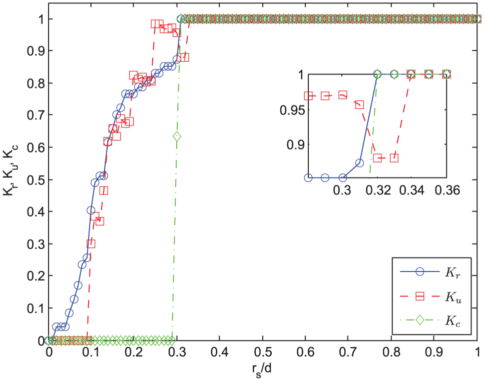
Next, we determined the $r_s/d$ values at which $K_r$ , $K_u$ , and $K_c$ attain the value of 1, so that $G$ becomes rigid, redundantly rigid, and 3-connected, respectively. Note that $K_u$ may become 1 before $G$ becomes rigid. This indicates that all the edges are redundant in the graph. But this is not what we are interested in. So, we imposed the condition that $K_r=1$ when $K_u$ attain the value of 1. This ensures that we determine the $r_s/d$ value for redundant rigidity. The resulting plot is shown in Figure 5.

Figure 5.

$r_s/d$ values at which $K_r$ , $K_u$ , and $K_c$ attain the value of 1 in random geometric graphs.

We make the following observations for random geometric graphs:

• In simulations (1, 10, 13, 22, 24, 32, 35, 37, 38, 44), first $K_r$ , then $K_u$ , and finally $K_c$ becomes 1.

• In simulations (2–9, 12, 14–21, 23, 25–31, 33, 34, 36, 39–43, 45, 47–50), first $K_r$ becomes 1, then $K_u$ and $K_c$ together become 1 at the same $r_s/d$ value.

• In simulation (11), $K_r$ and $K_u$ become $1$ at the same $r_s/d$ value; then, $K_c$ becomes $1$ .

• In simulation (46), $K_r$ , $K_u$ , and $K_c$ together become $1$ at the same $r_s/d$ value.

• We note that in none of the simulations, $K_c$ becomes $1$ before $K_u$ reaches this value.

Clustered graphs

Second, “clustered graphs” are considered in modeling sensor networks. When the distribution of nodes is not uniform, clustering, where the clusters are based on geographic location, becomes an issue to enable energy-efficient network operation. ³⁷ Clustering was also considered in the study of Marcelín-Jiménez et al. ³⁸ such that a network becomes more rigid by increasing connections between clusters. As in random geometric graphs, we assume that there are $n$ nodes on a $d\times d$ square area, and two vertices are connected by an edge if their distance is less than or equal to some given sensing range $r_s$ .

First, we give some additional definitions. A cluster $C_i$ is identified by subgraph induced by a node set as $G(C_i):=(C_i,E(C_i))$ , where $E(C_i):=\{(v,w)\in E:v,w\in C_i\}$ . Given a graph $G=(V,E)$ and $k\in {\mathbb{N}}_{>1}$ , a collection of vertex sets $C=\{C_1,C_2,\dots ,C_k\}$ , where $C_i\ne Ø$ for each $i$ , is a partition of $V$ , if $\bigcup _{i=1}^n{C}_i=V$ and $C_i\bigcap C_j=Ø$ for $i\ne j$ , such that each subgraph induced by the vertex set $C_i$ is connected. Each $C_i$ is called a $\mathrm{cluster}$ . The set $E_a:=\bigcup _{i=1}^{k}E(C_i)$ is called the set of intra-cluster edges, and $E_r=E\backslash E_a$ is called the set of inter-cluster edges. We refer the reader to the study of Gaertler ³⁹ for more details on graph partitioning and clustered graphs.

In simulations, we take $n=25\mathrm{units}$ and $d=30\mathrm{units}$ , as we did in random geometric graphs, for comparison purposes. An exemplary distribution of clusters is shown in Figure 6 (simulation 1).

Figure 6.

An exemplary clustered node distribution.

If we take the sensing radius $r_s=11.7\mathrm{units}$ , the resulting clustered graph is shown in Figure 7.

Figure 7.

The resulting clustered graph for the node distribution in Figure 6 when the sensing radius is 39% of the side length of the area.

There are four clusters, namely, $C_1,C_2,C_3,C_4$ . Each cluster in $(C_1,C_2,C_3,C_4)$ is confined in one of the four closed domains $(D_1,D_2,D_3,D_4)$ , respectively. The first cluster is distributed in the closed domain $D_1=\{(x,y):x,y\in [3,12]\}$ . The rest of the domains are as follows: $D_2=\{(x,y):x\in [18,27],y\in [3,12]\}$ , $D_3=\{(x,y):x\in [3,12],y\in [18,27]\}$ , $D_4=\{(x,y):x,y\in [18,27]\}$ .

For the same clustered distribution, we generated clustered graphs for several $r_s$ , taking values from $0$ to $d$ . As the sensing radius increases, $K_r(G)$ , $K_u(G)$ , and $K_c(G)$ do change. The values of $K_r(G)$ , $K_u(G)$ , and $K_c(G)$ are plotted against the ratio $r_s/d$ in Figure 8. In this plot, the node distribution in Figure 6 is used.

Figure 8.

When $r_s$ takes different values, $K_r(G)$ , $K_u(G)$ , and $K_c(G)$ do also change. Plots of $K_r(G)$ , $K_u(G)$ , and $K_c(G)$ against $r_s/d$ for the clustered node distribution in Figure 6.

As expected from Theorem 2 of Eren, ¹¹ $K_u(G)$ exhibits a non-monotonic behavior. When the edges in each cluster becomes a generalized redundant edge, $K_u(G)$ becomes $1$ although the entire graph is not redundantly rigid. As $r_s$ increases, new edges between clusters appear, which are not necessarily redundantly rigid, so $K_u(G)$ drops down. As more edges appear with an increasing $r_s$ , all the edges eventually become generalized redundant edges, and $K_u(G)$ attains the value of $1$ again. However, both $K_r(G)$ and $K_c(G)$ exhibit a non-decreasing behavior, again as expected from Theorem 2 of Eren ¹¹ and Theorem 1 of this article.

We repeated the computation of $K_r(G)$ , $K_u(G)$ , and $K_c(G)$ as a function of the ratio $r_s/d$ for $50$ different clustered distributions. Average values of $K_r(G)$ , $K_u(G)$ , and $K_c(G)$ as a function of the ratio $r_s/d$ , computed for 50 different node distributions, are shown in Figure 9.

Figure 9.

Average values of $K_r(G)$ , $K_u(G)$ , and $K_c(G)$ as a function of the ratio $r_s/d$ , computed for 50 different node distributions.

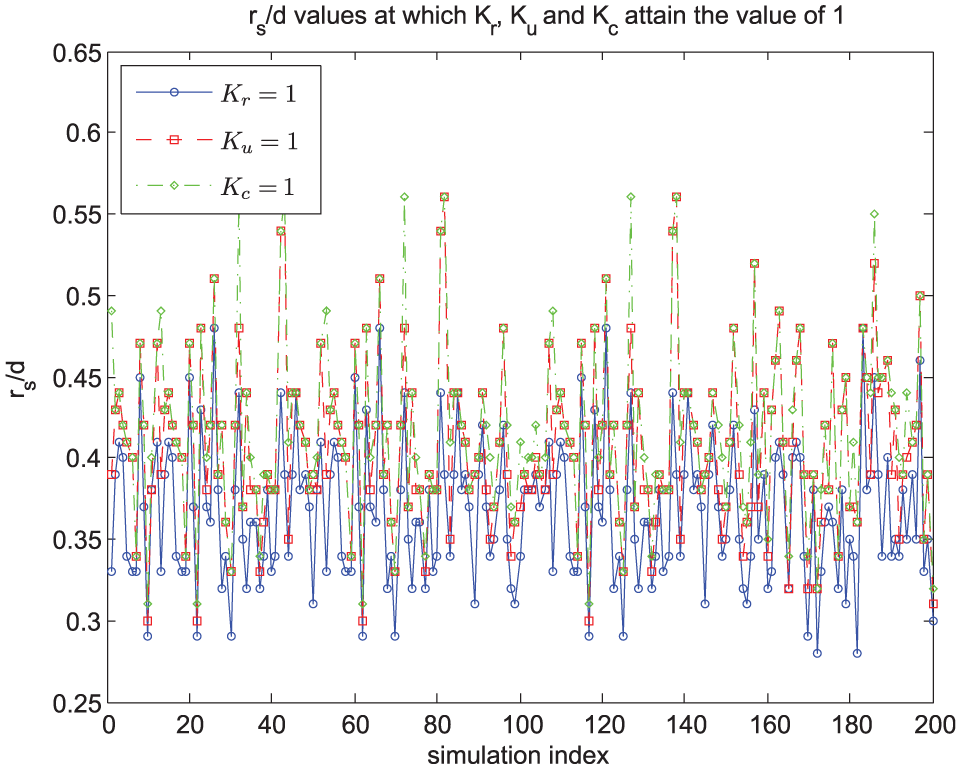
Then, we determined the $r_s/d$ values at which $K_r$ , $K_u$ , and $K_c$ attain the value of $1$ , so that $G$ becomes rigid, redundantly rigid, and 3-connected, respectively. As in random geometric graphs, we imposed the condition that $K_r=1$ when $K_u$ attain the value of $1$ to avoid the situations in which all edges are generalized redundant edges although the graph is non-rigid. This ensures that we determine the $r_s/d$ value for redundant rigidity. The resulting plot is shown in Figure 10.

Figure 10.

$r_s/d$ values at which $K_r$ , $K_u$ , and $K_c$ attain the value of $1$ in clustered graphs.

We make the following observations for clustered graphs:

• In simulations (1–3, 6, 16, 19, 21, 25, 26, 28, 30, 33, 40, 43, 49, 50), first $K_r(G)$ , then $K_u(G)$ , and finally $K_c(G)$ attain the value of $1$ . For example, the results of simulation (1) is shown in Figure 8.

• In simulations (4, 5, 9, 12, 13, 17, 20, 22, 23, 27, 34–37, 47, 48), $K_r$ reaches the value of $1$ first, then $K_u$ and $K_c$ become $1$ at the same $r_s/d$ value.

• In simulations (7, 8, 10, 14, 15, 18, 24, 31, 39, 44–46), first $K_r(G)$ and $K_u(G)$ together attain the value of $1$ , and then $K_c(G)$ attain the value of $1$ .

• In simulations (11, 32, 38, 41, 42), $K_r$ , $K_u$ , and $K_c$ all become $1$ at the same $r_s/d$ value.

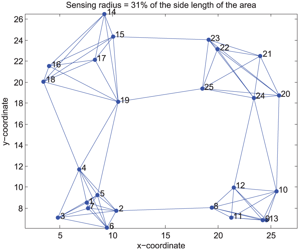
• Contrary to the behaviors observed in random geometric graphs, there is a noteworthy difference in clustered graph simulations. For the clustered node distribution shown in Figure 11 (simulation 29), if we take the sensing radius $r_s=9.3$ units, the resulting clustered graph is shown in Figure 12. Although this graph is 3-connected, it is not redundantly rigid, because if we remove any one of the edges in {(15, 23), (19, 25), (2, 8)}, the resulting graph becomes non-rigid. Therefore, for this distribution, first $K_r(G)$ , then $K_c(G)$ , and finally $K_u(G)$ attain the value of $1$ as shown in Figure 13.

Figure 11.

Another exemplary clustered node distribution.

Figure 12.

The resulting clustered graph for the node distribution in Figure 11 when the sensing radius is 31% of the side length of the area.

Figure 13.

When $r_s$ takes different values, $K_r(G)$ , $K_u(G)$ , and $K_c(G)$ do also change. Plots of $K_r(G)$ , $K_u(G)$ , and $K_c(G)$ against $r_s/d$ for the clustered node distribution in Figure 11.

Discussion

First, let us recall the questions that we posed in section “Introduction.” The first question was whether satisfying redundant rigidity or 3-connectivity is difficult once either of them is achieved, and in particular, what percentage increase in sensing radii is needed to reach from redundant rigidity to 3-connectivity, or vice versa.

In random geometric graphs, in simulations (1, 10, 11, 13, 22, 24, 32, 35, 37, 38, 44), $K_u$ becomes $1$ before $K_c$ reaches this value. In the rest of the simulations, $K_u$ and $K_c$ become $1$ at the same $r_s/d$ value. On average $2.38\%$ increase in $r_s$ is necessary to obtain a 3-connected graph from a redundantly rigid graph.

In clustered graphs, there was one exception where $K_c$ becomes $1$ before $K_u$ reaches this value (simulation 29). In all other simulations, $K_u$ becomes $1$ before $K_c$ reaches this value or they reach the value of $1$ at the same $r_s/d$ value. On average, $4.35\%$ increase in $r_s$ is necessary to obtain a 3-connected graph from a redundantly rigid graph.

We reach the conclusion that attaining 3-connectivity is considerably easy once redundant rigidity is achieved, for both random geometric graphs and clustered graphs.

Next, let us recall the other issue that we raised in section “Introduction,” specifically, the issue whether redundant rigidity implies 3-connectivity or vice versa.

Recall that for a graph $G$ to be global rigid, $G$ has to be redundantly rigid and 3-connected. An example, for which $G$ is redundantly rigid but not 3-connected is shown in Figure 14.

Figure 14.

An exemplary graph $G$ , for which $G$ is redundantly rigid, but not 3-connected.

The trapezoid composed of $v_2,v_4,v_5,v_6$ can reflect over the edge $(v_2,v_4)$ as shown in Figure 15.

Figure 15.

Partial reflection: the trapezoid composed of $v_2,v_4,v_5,v_6$ can reflect over the edge $(v_2,v_4)$ .

Therefore, the framework in Figure 14 is not congruent to the one in Figure 15, although they are equivalent. So, this framework is not globally rigid. Figures 14 and 15 are an example of partial reflection, and it can occur both in random geometric graphs and clustered graphs, which have unit disk connection structure, that is, proximity determines the neighbor relationship between the nodes in the network.

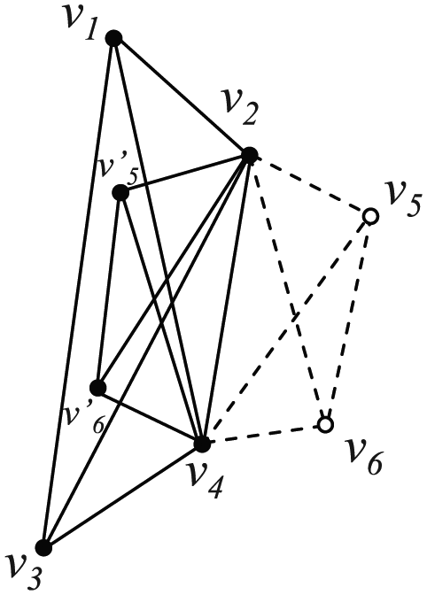
An example, for which $G$ is rigid, 3-connected, but not redundantly rigid is shown in Figure 16.

Figure 16.

An exemplary graph $G$ , for which $G$ is rigid, 3-connected, but not redundantly rigid.

A similar example was given in the study of Hendrickson ⁸ to demonstrate the necessity of redundant rigidity. Let us consider this graph as a bar-joint framework, where edges are solid bars connected by fully rotatable joints. If we remove the bar $(v_3,v_6)$ temporarily in Figure 16, then the triangle composed of $v_4,v_5,v_6$ can rotate on fully rotatable joints and move to $v{\prime }_4,v{\prime }_5,v{\prime }_6$ such that the length of $(v_3,v_6)$ is equal to the length of $(v_3,v{\prime }_6)$ . This is what we call discontinuous flexing as brought up in the study of Hendrickson ⁸ . Although the framework in Figure 16 is equivalent to the one in Figure 17, they are not congruent. Therefore, this framework is not globally rigid.

Figure 17.

Discontinuous flexing: if we remove the bar $(v_3,v_6)$ temporarily in Figure 16, then the triangle composed of $v_4,v_5,v_6$ can rotate on fully rotatable joints and move to $v{\prime }_4,v{\prime }_5,v{\prime }_6$ such that the length $(v_3,v_6)$ is equal to the length of $(v_3,v{\prime }_6)$ . Although the framework in Figure 16 is equivalent to the one in this Figure, they are not congruent.

Discontinuous flexing occurs in rigid graph clusters connected by few edges, which are inter-cluster edges. This is what happens for the framework in Figure 12 (simulation 29). When we temporarily remove the edge $(2,8)$ , two clusters on the right can rotate around the edges $(15,23),(19,25)$ , which result in discontinuous flexing. However, discontinuous flexing is less likely to occur in random geometric graphs with uniform distribution because it is less likely to have rigid components connected by inter-cluster edges to give rise to discontinuous flexing. We summarize as follows: (1) in random geometric graphs, a 3-connected graph is more likely to be redundantly rigid, that is, $K_c=1$ more likely implies $K_u=1$ ; (b) in clustered graphs, a 3-connected graph is not necessarily redundantly rigid, in other words, $K_c=1$ does not imply $K_u=1$ , so we need to check both 3-connectivity and redundant rigidity to make sure that they are both satisfied for global rigidity.

We may argue that 50 simulations are not sufficient in number to reach conclusions, and we wonder what happens if we increase the number of simulations. To respond to this concern, we increase the number of simulations to 200, for both random geometric graphs and clustered graphs. Then, we determine the $r_s/d$ values at which $K_r$ , $K_u$ , and $K_c$ attain the value of $1$ , so that $G$ becomes rigid, redundantly rigid, and 3-connected, respectively, in the same manner as we did for the case of 50 simulations. The resulting plot for random geometric graphs is shown in Figure 18. The results of 200 simulations are in agreement with our previous results of 50 simulations. In particular, we note that in none of the simulations, $K_c$ becomes $1$ before $K_u$ reaches this value.

Figure 18.

$r_s/d$ values at which $K_r$ , $K_u$ , and $K_c$ attain the value of $1$ in random geometric graphs with 25 nodes for 200 simulations.

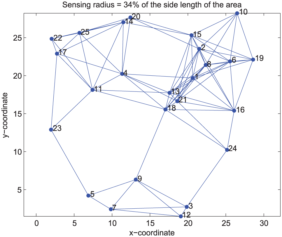
However, we still may question the existence of an exception, where $K_c$ becomes $1$ before $K_u$ reaches this value. To find this out, we increase the number of simulations to 1000. In only 1 simulation out of 1000 simulations (specifically, simulation 644), $K_c$ becomes $1$ before $K_u$ reaches this value. In particular, $K_c$ becomes $1$ at $r_s/d=0.34$ where $K_u<1$ . For this $r_s/d=0.34$ value, we plot the network in Figure 19. We observe that this graph is 3-connected; however, it is not redundantly rigid because if we remove any one of the edges in $\{(5,23),(9,18),(3,24)\}$ , the graph becomes flexible. The most noticeable feature of this graph is that the set of nodes $\{3,5,7,9,12\}$ actually forms a cluster $(C_1)$ within the graph, where the remaining 20 nodes form the other cluster $(C_2)$ , and $(5,23),(9,18),(3,24)$ are the inter-cluster edges connecting $C_1$ and $C_2$ . Therefore, the existence of clustering in a random geometric graph is the reason why discontinuous flexing occurs resulting $K_c=1$ while $K_u<1$ .

Figure 19.

Random geometric graph with 25 nodes (simulation 644) when the sensing radius is 34% of the side length of the area.

The resulting plot for clustered graphs is shown in Figure 20. The results of 200 simulations are again in agreement with our previous results of 50 simulations. Specifically, we note that in simulation 29, simulation 75, and simulation 130, $K_c$ becomes $1$ before $K_u$ reaches this value.

Figure 20.

$r_s/d$ values at which $K_r$ , $K_u$ , and $K_c$ attain the value of $1$ in clustered graphs with 25 nodes for 200 simulations.

Moreover, we may argue that 25 nodes is not large enough for a sensor network to reach conclusions, and we ask what happens if we increase the number of nodes. To answer this question, we increase the number of nodes to 200, for both random geometric graphs and clustered graphs. Exemplary networks for random geometric graph and clustered graph with 200 nodes are shown in Figures 21 and 22, respectively.

Figure 21.

An exemplary random geometric graph with 200 nodes (simulation 150) when the sensing radius is 15% of the side length of the area.

Figure 22.

An exemplary clustered graph with 200 nodes (simulation 75) when the sensing radius is 11% of the side length of the area.

Then, we determine the $r_s/d$ values at which $K_r$ , $K_u$ , and $K_c$ attain the value of $1$ , so that $G$ becomes rigid, redundantly rigid, and 3-connected, respectively, in the same manner as we did for the case of 25 nodes. The resulting plot for random geometric graphs is shown in Figure 23. The results of 200 simulations with 200 nodes are in agreement with our previous results of simulations with 25 nodes. In none of the simulations, $K_c$ becomes $1$ before $K_u$ reaches this value.

Figure 23.

$r_s/d$ values at which $K_r$ , $K_u$ , and $K_c$ attain the value of $1$ in random geometric graphs with 200 nodes for 200 simulations.

We note that when we increase the number of simulations for networks with 200 nodes, we still do not observe a network where $K_c$ becomes $1$ before $K_u$ reaches this value. However, this does not rule out the existence of an exception. Yet, we believe that such an exception can occur if a cluster forms within a random geometric graph, as we observed in Figure 19.

The resulting plot for clustered graphs with 200 nodes for 200 simulations is shown in Figure 24. The results of simulations with 200 nodes are again in agreement with our previous results of simulations with 25 nodes. Specifically, we note that in simulations with indices 31, 68, 75, 89, 98, 131, 148, 193, $K_c$ becomes $1$ before $K_u$ reaches this value. For example, (simulation 75) for $r_s=0.11$ is shown in Figure 22. We note that for the selected sensing radius, $K_c=1$ but $K_u<1$ in Figure 24. This can be verified from the network, that is, the graph in Figure 22 is 3-connected; however, it is not redundantly rigid because if we remove any one of the edges in {(42, 128), (120, 195), (146, 163), (57, 177), (63, 158)}, the graph is non-rigid; in fact, it is not even rigid with those set of edges.

Figure 24.

$r_s/d$ values at which $K_r$ , $K_u$ , and $K_c$ attain the value of $1$ in clustered graphs with 200 nodes for 200 simulations.

Conclusion

In this article, we introduced a graph invariant for3-connectivity that we termed the 3-connectivity index, $K_c(G)$ . This index results from the combinatorial connectivity properties of a graph. Using the 3-connectivity index along with the rigidity and redundancy indices, we explored the rigidity and connectivity properties of two classes of graphs, namely, random geometric graphs and clustered graphs.

Our previous work of Eren ¹¹ showed that it needs considerably less effort to obtain redundant rigidity once the network becomes rigid. In this article, we investigated the transition from redundant rigidity to 3-connectivity and vice versa. First, we have found out that, in random geometric graphs, it is considerably easy to achieve 3-connectivity once we obtain redundant rigidity. Specifically, redundant rigidity and 3-connectivity are either satisfied at the same $r_s/d$ (the ratio between the sensing radius, $r_s$ , and the side length of the area, $d$ ), or an average $2.38\%$ increase in $r_s/d$ converts a redundantly rigid graph into a 3-connected graph. It is worth noting that in random geometric graphs with uniform distribution, it is unlikely to observe a graph, in which 3-connectivity is satisfied before the graph becomes redundantly rigid. Therefore, in random geometric graphs, it is more likely sufficient to test only 3-connectivity for unique localizability. We discuss that this is related to the lack of occurrence of discontinuous flexing in random geometric graphs.

Second, we have found out that in clustered graphs, redundant rigidity and 3-connectivity are either satisfied at the same $r_s/d$ or an average $4.35\%$ increase in $r_s/d$ converts a redundantly rigid graph into a 3-connected graph. Moreover, on the contrary to random geometric graphs, our findings indicate that in clustered graphs,3-connectivity may be satisfied before the graph becomes redundantly rigid because it is possible to have rigid components connected by inter-cluster edges, which may result in discontinuous flexing. Therefore, in clustered graphs, we have to test both redundant rigidity and 3-connectivity for unique localizability.