
Abstract
In wireless sensor networks, time synchronization is an important issue for all nodes to have a unified time. The wireless sensor network nodes should cooperatively adjust their local time according to certain distributed synchronization algorithms to achieve global time synchronization. Conventionally, it is assumed that all nodes in the network are cooperative and well-functioned in the synchronization process. However, in cognitive radio wireless sensor networks, the global time synchronization process among secondary users is prone to fail because the communication process for exchanging synchronization reference may be frequently interrupted by the primary users. The anomaly nodes that failed to synchronize will significantly affect the global convergence performance of the synchronization algorithm. This article proposes an anomaly node detection method for distributed time synchronization algorithm in cognitive radio sensor networks. The proposed method adopts the statistical linear correlation analysis approach to detect anomaly nodes through the historical time synchronization information stored in local nodes. Simulation results show that the proposed method can effectively improve the robustness of the synchronization algorithm in distributed cognitive radio sensor networks.
Keywords
Introduction
Wireless sensor network (WSN) is a special distributed wireless network that can support pervasive and robust monitoring of various physical conditions such as temperature, sound, humidity, and so on. Designed for rapid and robust deployments, WSNs are widely used in both military and civilian applications. 1 Time synchronization plays a very important role in WSNs because it enables all nodes to have a unified time, on which all applications such as data collection and environment monitoring depend.1,2 Cognitive radio (CR) network has been widely regarded as a key technology to increase the spectrum utilization of wireless communication systems. 3 CR technology enables secondary users (SUs) without spectrum license to share wireless channels with primary users (PUs) who hold the spectrum license through dynamic spectrum access technology. The application of CR technology in WSNs can enhance the capacity of WSNs and has been widely investigated in recent years.4,5 However, time synchronization in cognitive radio sensor networks (CRSNs) is prone to failure because the communication process for exchanging synchronization references among SUs may be frequently interrupted by the PUs’ activity. The anomaly nodes that fail to keep synchronized will significantly reduce the convergence performance of the synchronization algorithm in CRSNs. 4
In the literature, many-time synchronization algorithms for WSNs have been proposed. These algorithms can be broadly categorized into two types: centralized and distributed approaches. 1
In the centralized approach, there is a powerful central node servicing as a root. The root node and other nodes in the network form a tree or mesh topology. The central node periodically broadcasts the time reference information, marked as level 1. Based on the received level 1 timing information, the neighbor nodes of the root adjust their local time references and marked them as level 2. In the same way, the two-hop neighbor nodes of the root adjust their local time reference according to the root node’s one-hop neighbors. The same procedure propagates through the entire network. If a node receives more than one timing references from its neighbor nodes, it will adjust its local time reference according to the node with the most superior level.6–10 The centralized methods are effective in achieving the convergence of time synchronization with a low signaling cost. In addition, it is easy to find an abnormal node that does not adjust its local time reference. However, these centralized algorithms are over-dependent on the root node. Moreover, the time reference bias and error will accumulate as the hops between a node and the root node increase. Therefore, distributed synchronization algorithms are proposed.
In the distributed approach, each node independently adjusts its time reference according to the time difference between its local time reference and the time reference of its neighbor nodes. In the literature, different types of the distributed algorithms have been proposed. The major types are test-based detection, majority voting detection, and node–self-detection methods.
In the test-based detection methods, nodes execute test task and then make a judgment on abnormal nodes based on the test results. In a k-connected graph, Webber let one node execute the test together with its neighbors to detect the abnormal node. 11 This algorithm requires that every node should have a given number of neighbors, so its application is restricted to some limited scenarios. Chessa proposed a test-based algorithm using comparison method.12,13 In his algorithm, the system will choose a trusted node to broadcast test information. Its neighbors, respectively, compare the information and then return a testing result to the trusted node for deciding if a node is normal or not. This algorithm is suitable to distributed networks, but how to choose a trusted node becomes a new problem. On the basis of Chessa’s algorithm, Elhadef proposed some improved algorithms—adaptive Distributed Self-Diagnosis Protocol (DSDP) and mobile DSDP. 14 Similar methods of regularly checking nodes’ behavior in WSNs to detect abnormal nodes were discussed in You et al. 15 and El-Koujok et al. 16 Although the test-based algorithms can improve the detection accuracy, they also bring challenges in terms of the communication cost and computational complexity.
The majority voting detection method takes the advantage of the spatial similarity of the nodes in WSNs to decide abnormal nodes. Vuran et al. 17 set a threshold value to test the difference between two nodes. If the difference is higher than the threshold, one of the two nodes is likely to be abnormal. If one node is voted by all its neighbors, the node will be regarded as an abnormal node. As an improvement to the simple voting, the voting methods discussed in Xiao et al. 18 and Behnke et al. 19 were affected by the weights between nodes. The method presented in Xiao et al. 18 required that the nodes be connected only when they are similar, which make the voting credible. The Efficient Localized Detection of Erroneous Nodes (ELDEN) proposed by Behnke et al. 19 computed the weight through the distance between nodes and every node chooses the median of its neighbors to compare with its own state value. Then the difference will be normalized by the weight and becomes the final difference Y. If Y is higher than the threshold, a node is regarded as abnormal. The majority voting detection method can achieve a good performance in accuracy with a relatively small signaling cost, but it shows a poor performance in scenarios with a small number of nodes.
The node–self-detection methods for distributed WSNs were discussed in Babaie et al.;20–22 these algorithms require extra hardware or software to complete the detection, which impose extra cost for resource limited nodes in WSNs.
Through the above literature review, we can find that detecting the abnormal nodes in distributed time synchronization is very important for cognitive WSNs. The abnormal nodes who could not adjust its local time reference according to the time synchronization algorithm will damage the convergence of the algorithm. In this article, we propose a novel method to detect the abnormal node in distributed time synchronization algorithm. In our method, the correlation coefficient is introduced to compute the local time reference correlation between nodes in the networks. As the time reference of an abnormal node is likely to be uncorrelated to the time reference of the normal node, the correlation coefficient can be used as a metric for effective detection of abnormal nodes in the network.
System model
In this article, we study the time synchronization algorithm under an assumption that the topology of the cognitive WSN is a totally connected graph. Messages sent from a source node will successively be received by any given destination node in the network within several hops. All the nodes except the abnormal nods in the network adjust their local time references according to the distributed synchronization algorithm.
Distributed synchronization algorithm
The algorithm proposed in this article is designed for WSNs in which nodes communicate in a distributed manner. We denote the set of all points/network nodes as

Here,
The weights between non-neighbor nodes which do not belong to
The distributed time synchronization algorithm can be expressed as

Here,
Synchronization error model
Assume that an abnormal node appears in the network, whose state of time reference does not change according to the distributed synchronization algorithm. The existence of abnormal node will influence time reference of its neighbor nodes in the next iteration of the synchronization algorithm, such that its neighbor nodes will have incorrect time references. These neighbor nodes with error time references will further influence their nearby nodes to get incorrect time references. The error of time reference will propagate as the algorithm iterates, which is shown in Figure 1.

The spread of error information.
Supposed that the node

In equation (4), the time reference of all the normal nodes expect the abnormal node change according to equation (2). As the existence of abnormal node will affect the time reference of other nodes in the network, we should study the convergence problem of the synchronization algorithm.
If there are more than two abnormal nodes which do not change their time references in the network—all other
Assumed that node
Correlation coefficient
According to the synchronization error model, all the normal nodes current state of time reference are computed by the distributed average of their neighbors’ previous state of time reference. Thus, the time reference of a normal node will linearly correlate to that of their neighbor nodes. However, the time reference of the abnormal node is independent from those of its neighbors, since it does not adjust its local time reference according to the synchronization algorithm. The main idea of the proposed abnormal node detection method is that every node should compare the correlation coefficient between the local time reference and that of its neighbors.
In statistics, there are several tools to analyze the correlation between two sample groups, such as Pearson product–moment correlation coefficient (PPMCC), Spearman’s correlation coefficient for ranked data, and the Kendall coefficient of concordance. These tools have different usage scenarios; we choose PPMCC in this article because PPMCC is a good metric for measuring the linear dependence.
PPMCC is a frequently used tool in statistics; it is used to measure the linear correlation between two variables. The correlation value of PPMCC ranges from −1 to 1. If the value is larger than 0, it means that the two variables measured are positively correlated. Otherwise, they are regarded as negatively correlated. If the value is close to 0, it means the two variables are uncorrelated.
The PPMCC of two continuous variables is defined as the quotient of their covariance and standard deviation, that is

Here,


The standard deviations are expressed in equation (8)

Therefore, the covariance can be evaluated as

The correlation coefficients of the time reference of nodes in WSNs, which is expressed in equation (9), are used as the parameter to detect the abnormal nodes.
Algorithm description
In this article, we assume that the topology is static and there is one abnormal node at most. As Figure 2 shows, the algorithm consists of two forms: non-real-time detection and real-time detection. The former is used to find out the abnormal node when the network has been un-synchronized, which needs less computation cost. The latter is working with synchronization algorithm to monitor the network and detect the abnormal node.

Algorithm flowchart: (a) non-real-time detection and (b) real-time detection.
Non-real-time detection
The non-real time detection algorithm is shown in Figure 2(a). In this form, the network is un-synchronization. Then the follow steps are used to find out the abnormal node:
Execute the synchronization algorithm N times according to equation (4), and each node stores the local time reference states in a sequence.
Each node computes the coefficient of time reference between itself and its neighbors by the PPMCC method. Because node
After computing the PPMCC, every node chooses its neighbor node whose correlation coefficient is the smallest and notices the chosen node that it has a problem. If one node is noticed by all its neighbors, the node will be regarded as a suspected abnormal node.
If there is only one suspected abnormal node, the node been chosen is confirmed as the abnormal node. If there exists more than one suspected abnormal nodes, they will compute their autocorrelations, respectively (its buffer from 1 to
Real-time detection
The real-time detection is shown in Figure 2(b). In this scenario, the network has been synchronized, and the algorithm is used to monitor whether one normal node becomes abnormal suddenly. Every node has a
Before the abnormal node appears, the nodes execute the synchronization algorithm, update the buffers, and compute the PPMCC:
If the PPMCCs of node
If there exists only one suspected abnormal node, its disable node list will plus 1. If there are several suspected abnormal nodes, we will do it by the same way which non-real-time detection does in step 4.
The node selected as the final suspected abnormal node will plus its disable node list, and the other suspected abnormal nodes’ disable node list will reset.
If one node’s disable node list comes to be
Feasibility analysis
As mentioned previously, the abnormal node is like a virus, it will spread error information to its neighbors, and the neighbors will also spread the error information to their nearby nodes.
In Figure 3, the strength of the influence from the abnormal node is shown. Darker color means the nodes suffer more influence from the abnormal node. Similarly, the number shown between two nodes indicates the strength of their PPMCC. The larger the number, the weaker the correlation coefficient. Since one node will have weak linear dependence with its neighbors if it is much affected by the abnormal node, the node will be selected as the problematic node with a higher probability.

Influence of abnormal node.
Therefore, the abnormal node will surely be selected as the suspected abnormal node in this way. However, one of the abnormal node’s neighbor also has the probability to be selected as the suspected abnormal node, because the abnormal node also chose one of its neighbor to notice as the abnormal node. If one node is noticed by the abnormal node as an abnormal node, and it is also noticed by other neighbors at the same time, the node will be another suspected abnormal node. In this way, there will be two suspected nodes at most: one of them is the abnormal node, and the other one is its neighbor.
If there exists two suspected abnormal nodes, we just need to compute the autocorrelation value. Because the next state of time reference in one normal node contains the information of the current state of time reference, the time reference of the abnormal node is uncorrelated to its previous state. The node with weaker autocorrelation can be confirmed as the abnormal node.
If the degree of abnormal node is 1, its only neighboring node will find that the correlation coefficient with the abnormal neighboring node is lower than that with another normal neighboring node. Hence, the abnormal node will be detected. If a normal node connects to the network only by an abnormal node, its time reference is adjusted by that of the abnormal node. The time reference of the normal node may be incorrect because the abnormal node is its only neighboring node. However, it does not affect other nodes in this circumstance, because the normal node with incorrect time reference does not have neighbor of any other normal nodes. Therefore, adopting the statistical linear correlation analysis approach is an effective method to detect anomaly nodes.
Simulation and results
In this article, we simulate in a normalized 1 × 1 square area. In the simulation area, there are
Non-real-time detection
Non-real-time detection is used to find out the abnormal node when the network has been un-synchronized.
Length of buffer B
The non-real-time scenario, the abnormal nodes detection algorithm was run one time to discover the influence of length of buffer to the detection rate, is marked as “once detection” in Figure 4.

The influence of the length of buffer
In Figure 4, we can find that the length of buffer
Besides, we can find that the result with less nodes is better than the result with more nodes when the buffer is fixed.
Node density N
The relationship between the node density and the detection rate is shown in Figure 5.
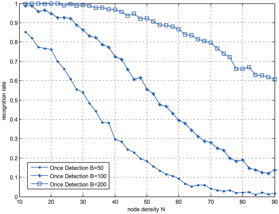
The influence of the node density
As Figure 5 shows, when the length of buffer is fixed, with the node density
On the other hand, with the whole node density
Real-time detection
Real-time detection is working with synchronization algorithm to monitor the network and detect the abnormal node.
Length of buffer B
In real time detection scenario, we need to observe the iteration time which began from the abnormal node appears until it has been detected. We call the iteration time as the cost. In the real-time scenario, the influence of length of buffer to the detection rate is shown in Figure 6.

The influence of the length of buffer
Comparing Figure 6 with Figure 4, we can find that the real-time detection method is more efficient than the non-real-time detection method. When node density and communication radius are fixed, real-time detection can reach the same performance with less buffer demand. In real-time detection, the abnormal node is immediately detected when it appears, where most of the nodes in the network, except the abnormal node and its neighbor nodes, are still in synchronization. Hence, the error information from the abnormal node has not been widely spread and it will be easier to detect the abnormal node with less time reference samples.
The influence of the length of buffer

The influence of the length of buffer
It is seen from Figure 7 that the real-time detection method requires more computation cost, with the buffer increasing, and the cost of time to detect the abnormal node would decline.
Node density N
The influence of the node density

The influence of the node density
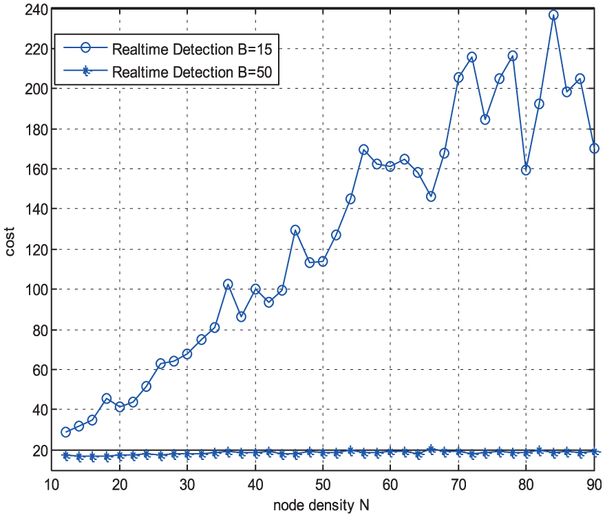
The influence of the node density
From Figures 8 and 9, we can find that when the length of buffer is not large enough, the abnormal node’s detection rate and computation cost will all decline as the node density increases. The reason is that the weight value in the distributed time synchronization algorithm declines when the node density increases; thus, the correlation value of time reference between neighbor nodes will be smaller. Therefore, more iteration time is required to achieve the detection.
Conclusion
In this article, a novel distributed time synchronization algorithm has been proposed for CRSNs. The proposed algorithm can effectively detect the abnormal nodes that fail to comply with the normal synchronization behavior. Our algorithm relies on a key insight that the time reference trace of the abnormal node tends to be linearly uncorrelated with its neighboring nodes. This insight is used to design a voting and consensus mechanism to detect abnormal nodes using linear correlation as a metric. Simulation results show that the proposed method can effectively detect the abnormal node in CRSNs in both the non-real-time and real-time scenarios.
Footnotes
Handling Editor: Katsuya Suto
Declaration of conflicting interests
The author(s) declared no potential conflicts of interest with respect to the research, authorship, and/or publication of this article.
Funding
The author(s) disclosed receipt of the following financial support for the research, authorship, and/or publication of this article: The authors would like to acknowledge the support of the China Scholarship Council (CSC) and the Natural Science Foundation of China (NSFC, nos 61201196, 61601388, 61571378, and 61371081).