Sage Journals: Discover world-class research

Abstract

Node localization plays a key and basic role for wireless sensor network. Existing range-free localization approaches suffer from precision limit of positioning, while range-based solutions may obtain good accuracy but pay high costs for ranging hardware. Instead of directly mapping received signal strength values into physical distances, a novel localization scheme with signal-based signature distance estimation is proposed for wireless sensor network. More specifically, we first quantify the near-far relationship between neighbor nodes through received signal strength comparison, and then the distance between non-neighbor nodes is calculated by an improved shortest path algorithm. Based on the obtained node distance, a relative map can be constructed by multidimensional scaling technology. Eventually, the locations of nodes can be acquired by virtue of Procrustes analysis method. For purpose of verifying the effectiveness of our design, several simulations are made in a sensor network with 200 randomly deployed nodes, and two experiments are implemented in real outdoor environments: a linear network and a two-dimensional grid network with 25 nodes. It is remarkable from results that the proposed scheme performs better in positioning and reduces localization errors by as much as 37% compared with state-of-the-art methods.

Keywords

Range-free localization signal-based signature distance wireless sensor networks

Introduction

Wireless sensor network (WSN), which consists of autonomous sensors, is an important technology to monitor the physical world, for example, indoor localization,¹ environment monitoring,² battlefield surveillance,³ item tracking⁴. In such data-driven WSN, the location is essential information. Besides, some of the routing protocols⁵ and data forwarding mechanisms are built on the assumption that nodes’ location information is available. Although node localization makes fundamental contributions to many applications, it still remains a challenging problem due to the limitation of low-cost and tiny nodes.

There currently exist many excellent localization algorithms in WSN. The first type is range-based localization, in which the ranging is completed by the received signal strength (RSS), time, or angle. In practice, these types of approaches are often accompanied by higher localization accuracy, while may not meet the demand of low-cost system design. The second one is range-free localization, in which wireless connectivity,⁶ anchor proximity,⁷ or localization events detection are adopted for location estimation. These algorithms have low cost but suffer from poor accuracy. Lately, another localization technology is proposed which is based on the channel status information (CSI).⁸ Such methods provide better positioning accuracy, but the CSI is often hard to extract for the general sensor nodes.

Our work is motivated by the finding that the change trend of the RSS values from their neighbors is similar if two nodes are placed near each other. Based on the observation, in this article, we further quantify the near-far relationship between neighboring nodes from two aspects: neighbor pair comparison and RSS difference. After obtaining the relative distance between neighboring nodes, the relative distance among non-neighboring nodes can be calculated by an improved shortest path algorithm. Thus, we can construct the relative location map of the whole network based on the multidimensional scaling (MDS) technology.⁹ Finally, given at least three anchors, the physical coordinates can be solved by Procrustes analysis. Specifically, our main contributions are as follows:

Different from the traditional hop-based distances, this article investigates the proximity information embedded in neighborhood RSS, which owns a more accurate sub-hop resolution.

The near-far relationship between neighbor nodes is carefully quantified based on neighbor pair comparison and nodes’ RSS difference, which has a high correlation with physical distance.

Instead of directly using the shortest path algorithm, this article explores the angle relationship between neighbors and adopts an integral calculation method to obtain the distance among non-neighbor nodes.

Extensive simulations and two experiments with 25 nodes are conducted for verifying the effectiveness.

The rest of the article is organized as follows: Section “Related work” surveys the related work about the localization. Section “Motivation” describes the motivation with empirical data. The main design is introduced in section “System design.” Section “Simulation” gives the simulation results and section “Experiments” reports the prototype outdoor experiments. Finally, section “Conclusion” concludes the article.

Related work

Generally, the localization approaches can be classified into three categories:¹⁰ range-based,^11,12 range-free,^7,13–15 and CSI-based.¹⁶ In the following, we will analyze and discuss them one by one.

Range-based methods can be further divided into three types: RSS-based methods,¹⁷ which convert the signal strength into distance by virtual of logarithmic attenuation model. The direct converting of RSS using the model is always inaccurate, due to the unknown radio path loss factors, multi-path effects, hardware discrepancies, antenna orientation, and so forth. Time-based methods like time of arrival (TOA),¹⁸ time difference of arrival (TDOA),¹⁹ round-trip time of flight (RTOF), and so on, calculate the distance based on the arrival time and radio transmitting speed. Such localization solutions often require high precision timer. Angle-based methods, like angle of arrival (AOA),²⁰ locate the tag by measuring the phase difference at different antennas. Those methods generally first estimate distances or angles among nodes and then calculate positions by triangulation. Due to per-node additional hardware or intensive tuning, range-based methods could achieve good performance in localization accuracy, but may pay higher price on system cost.

Range-free solutions try to estimate node location through a low-cost and smart design. There are three stages. Early solutions mainly employ the proximity information to anchor nodes like centroid²¹ and approximation point-in-triangulation test (APIT).²² These methods, however, often require a high anchor density for the sake of good localization accuracy. In the second stage, many localization solutions with wireless connectivity are proposed, such as distance vector-hop (DV-Hop), multidimensional scaling-map (MDS-MAP), amorphous. Given the hop-based distances among nodes, such methods only require a small number of anchors for constructing the global coordinates, which significantly reduces the cost. In the third stage, there are some works that help solve problems of holes²³ in practical irregular deployment with obstacles. We note that although the above works are effective, they do not fully extract the location information available from local neighborhood sensing.

Lately, the CSI-based localization strategies are proposed like SAIL²⁴ and Tagoram.²⁵ They utilize physical layer information to compute the propagation delay of the straight path, eliminating the adverse effect of multi-path and yielding sub-meter distance estimation accuracy. The adopted wireless technologies are WiFi or radio frequency identification (RFID). Although CSI is a better choice for distance estimation in many scenarios, it is hard to be extracted for low-cost sensors.

Considering that RSS can indeed provide more than just connectivity information among neighboring node pairs, but also other useful distance information, this article fully extracts the proximity information from the neighbors’ RSS and presents a novel method of quantifying the distance among neighbors. The design can effectively improve the system accuracy with little extra cost.

Motivation

Our work is motivated by one of outdoor experiments. We have ever constructed a two-dimensional grid network with a $4 \times 4$ layout including 16 nodes on a platform. The grid distance between two nodes is about 5 m. Each node records all the RSS values from their neighbors. After obtaining the RSS values, we plot the relationship between distances and RSS values, as shown in Figure 1. It can be seen that an identical RSS value may map multiple physical distances, and RSS may vary dramatically for a single distance. Thus, the direct converting from the RSS to the distance is inaccurate.

Figure 1.

RSS versus distance.

In view of this, we change the observation method of RSS values. From the viewpoint of a single node, there is another phenomenon. Figure 2 depicts the line charts recording all RSS values from a single node to the rest of other nodes in sequence, which is denoted as RSS change trend. Then, we attempt to compare the distinction of RSS change trends between closer node pair (nodes 1 and 2) and farther node pair (nodes 1 and 8). As shown in Figure 2, node 1 and node 2 almost have the similar RSS change trend, while there exist many inverse trends of RSS values for node 1 and node 8. This intuitive phenomenon inspires us to further extract the distance relationship behind the RSS change trend, and the latter simulations and experiments will verify the effectiveness of proposed design.

Figure 2.

RSS change trend among closer and farther node pairs: (a) RSS change trend of nodes 1 and 2 and (b) RSS change trend of nodes 1 and 8.

System design

The whole system design is shown in Figure 3. Based on the RSS values collected from physical layer, this section first presents the main design of quantifying the near-far relationship among neighboring nodes. Next, an integral approach is designed to accumulate relative distances among multi-hop node pairs. Then, the section describes the construction process of relative map of the whole network. Finally, the converting procedure of the physical coordinates is given in the last part.

Figure 3.

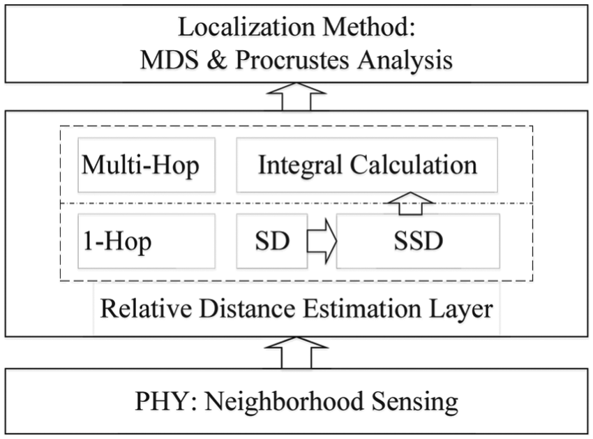
The localization system architecture.

Relative distance quantization

Sequential distance estimation

Without loss of generality, we can evaluate the near-far relationship of neighboring nodes $s_{1}$ and $s_{2}$ using the data group $G = (S, T, M)$ , where $S = {s_{1}, s_{2}}$ , $s_{1}$ and $s_{2}$ are the target objects for distance quantization; $T = {t_{1} (s_{1}), t_{2} (s_{2}), t_{3}, \dots, t_{N}}$ , which is a set that contains $s_{1}$ and $s_{2}$ , as well as all their neighbors. It is not difficult to obtain that there are $C_{N}^{2}$ neighbor pairs for nodes $s_{1}$ and $s_{2}$ , where $N$ is the total number of neighbors of the two nodes. $M$ is a $2 \times N$ matrix, in which $M_{ij}$ represents the RSS from node $t_{j}$ for node $s_{i}$ .

In order to illustrate our design, we give a simple example in Figure 4, in which the problem is to evaluate the distance between $s_{1}$ and $s_{2}$ . Table 1 lists the RSS values from all their neighbors. Note that if $M_{ij}$ is set to be $\infty$ , it means that node $s_{i}$ cannot receive the signal from node $t_{j}$ . In addition, we set $M_{ii}, i \in {1, 2}$ to be zero, which has the strongest signal strength.

Figure 4.

An example of relative distance quantization.

Table 1.

RSS values from all their neighbors (dBm).

Neighbors Objects	$t_{1} (s_{1})$	$t_{2} (s_{2})$	$t_{3}$	$t_{4}$	$t_{5}$	$t_{6}$	$t_{7}$	$t_{8}$
$s_{1}$	0	−59	−76	−81	−55	−57	$\infty$	$\infty$
$s_{2}$	−61	0	$\infty$	$\infty$	−59	−56	−58	−57

Now we classify the neighbor pairs of nodes $s_{1}$ and $s_{2}$ . For each neighbor pair, if $s_{1}$ and $s_{2}$ can both determine that one neighbor is closer than the other to themselves, such as node pair ( $t_{5}$ , $t_{6}$ ), we define this neighbor pair as an effective neighbor pair and use $N_{val}$ to denote the number of valid neighbor pairs. In contrast, $s_{1}$ cannot judge whether it is closer to node $t_{7}$ than $t_{8}$ , because it receives nothing from them. We call $t_{7}$ and $t_{8}$ as an invalid neighbor pair. Likewise, $s_{2}$ cannot judge whether it is closer to node $t_{3}$ than $t_{4}$ . Hence, $t_{3}$ and $t_{4}$ is also an invalid neighbor pair. To sum up, if $s_{1}$ or $s_{2}$ cannot determine which neighbor is closer to itself, we consider this neighbor pair as invalid neighbor pair. Here, $N_{inv}$ is used to represent the number of invalid neighbor pair. Obviously, the sum of $N_{val}$ and $N_{inv}$ equals to $C_{N}^{2}$ .

Next the distance estimation between nodes $s_{1}$ and $s_{2}$ is mainly based on the $N_{val}$ valid neighbor pairs. For any valid neighbor pair $t_{j}$ and $t_{k}$ , it is a ordered pair if $M_{1 j} > M_{1 k}$ and $M_{2 j} > M_{2 k}$ (or $M_{1 j} < M_{1 k}$ and $M_{2 j} < M_{2 k}$ ). Otherwise, if there exists an inverse RSS change trend, in other words, if the valid neighbor pair meets the conditions $M_{1 j} > M_{1 k}$ and $M_{2 j} < M_{2 k}$ (or $M_{1 j} < M_{1 k}$ and $M_{2 j} > M_{2 k}$ ), we consider $t_{j}$ and $t_{k}$ as a unordered pair. In the given example, nodes $t_{5}$ and $t_{7}$ constitute an unordered pair, while $t_{3}$ and $t_{5}$ form an ordered pair. In addition, we use symbols $N_{ord}$ and $N_{uno}$ to represent the number of ordered pairs and unordered pairs, respectively. Based on the above classification and explanations, we quantify the relative distance between nodes $s_{1}$ and $s_{2}$ as follows.

Definition 1

The sequential distance (SD) between two neighboring nodes is equal to the ratio between the number of discordant pairs and the number of effective neighbor pairs, namely

S D (s_{1}, s_{2}) = \frac{N_{u n o}}{N_{v a l}} {\begin{matrix} N_{u n o} = N_{v a l} - N_{o r d} \\ N_{v a l} = C_{N}^{2} - N_{i n v} \end{matrix}

(1)

Taking $s_{1}$ and $s_{2}$ in Figure 4 as an example, we can obtain 14 unordered pairs $(t_{1}, t_{2})$ , $(t_{1}, t_{5})$ , $(t_{1}, t_{6})$ , $(t_{1}, t_{7})$ , $(t_{1}, t_{8})$ , $(t_{2}, t_{5})$ , $(t_{2}, t_{6})$ , $(t_{3}, t_{7})$ , $(t_{3}, t_{8})$ , $(t_{4}, t_{7})$ , $(t_{4}, t_{8})$ , $(t_{5}, t_{6})$ , $(t_{5}, t_{7})$ , $(t_{5}, t_{8})$ and 2 invalid neighboring pairs $(t_{3}, t_{4})$ , $(t_{7}, t_{8})$ . Thus, the SD between nodes $s_{1}$ and $s_{2}$ is $14 / (C_{8}^{2} - 2) \approx 0.58$ .

We use the ratio of unordered neighbor pairs for evaluating the node distance. SD reflects a relation that the more inverse RSS change trends two neighbor nodes have, the farther away these two nodes are, which accords with the phenomenon mentioned above. In addition, we can also learn from the example above that the SD between a neighboring node pair can be obtained through $C_{N}^{2}$ comparative calculations. Therefore, the complexity of $SD (s, t)$ is $O (N^{2})$ .

Furthermore, we explore the hidden geometrical relationship behind equation (1). We consider any two neighboring nodes and draw a perpendicular bisector to the line connecting their positions. This perpendicular bisector divides the localization space into two different regions that are distinguished by their proximity to either neighboring node. In the same way, if perpendicular bisectors are drawn for all the $C_{N}^{2}$ neighboring pairs, they divide the localization space into many small regions. If nodes $s_{1}$ and $s_{2}$ are on different sides for many bisectors, they should be far from each other. Figure 5 illustrates the above-mentioned phenomenon. Nodes $A$ and $C$ are close with each other and lie on the same side for most bisectors. However, nodes $A$ and $B$ lie on the different sides for most bisectors and their distance is farther.

Figure 5.

Nodes with bisectors.

Signal-based signature distance estimation

In the above analysis, we only consider the change trend of RSS. However, the RSS values can also inflect the distance between two nodes, especially in the outdoor open-air scenarios. Next, we further introduce the differences of neighbor RSS values into the relative distance estimation.

For nodes $s_{1}$ and $s_{2}$ , the difference-based distance can be expressed as equation (2) with the complexity of $O (N)$

d_{d i f f} (s_{1}, s_{2}) = \sum_{i = 1}^{N} | M_{1 i} - M_{2 i} |

(2)

Note that in equation (2), the RSS differences are used to estimate the distance instead of RSS values, which can in part eliminate the effect of the environment factor and is more robust. Based on the SD and difference-based distance, we propose a signal-based signature distance (SSD) for relative distance between one-hop neighboring nodes.

Definition 2

SSD between a one-hop node pair is equal to the product of the SD and a polynomial based on the difference-based distance, which is shown as follows

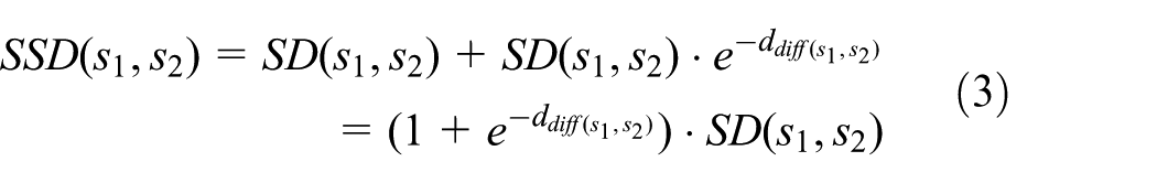
\begin{matrix} SSD (s_{1}, s_{2}) = SD (s_{1}, s_{2}) + SD (s_{1}, s_{2}) \cdot e^{- d_{diff (s_{1}, s_{2})}} \\ = (1 + e^{- d_{diff (s_{1}, s_{2})}}) \cdot SD (s_{1}, s_{2}) \end{matrix}

(3)

From equation (3), it can be seen that SSD combines the ideas of RSS differences ( $d_{diff}$ ) and RSS change trend ( $SD$ ), which makes up for the weakness of using one aspect only and enhances the robustness. Moreover, according to the previous analysis, it can be easily obtained that the complexity of $SSD$ is $O (N^{2})$ .

The rational behind the equation is that we employ the RSS differences to correct the SD. Since the values of RSS differences are relative large, directly integrating them into the SD will bring extra errors. Hence, we adopt the widely used exponential form to construct a new distance metric. Thus, the distance is jointly determined by the sequence of neighbor nodes, as well as the RSS difference of one node itself.

SSD integral calculation

In last subsection, we start from the concepts of neighboring node pairs and their RSS change trends and then quantify the SD and propose SSD based on comparison of RSS values and RSS differences. However, SD and SSD can only reflect the near-far relationship between two neighboring nodes. As for non-neighboring node pairs, there will be a exploration about an existing approach, as well as an introduction of an integral method for calculation of relative distances between two non-neighbor nodes.

The existing design of regulated signature distance (RSD)²⁶ uses the smallest accumulated RSD along a path between two nodes instead of the shortest path hop-count as the estimated relative distance. If we draw on the experience of RSD, the relative distance between two non-neighbor nodes is the addition of SSD along the shortest path from one node to the other. Taking Figure 6(a) as an example, the relative distance between $s_{2}$ and $t_{3}$ equals to the sum of $SSD (s_{1}, s_{2})$ and $SSD (s_{1}, t_{3})$ .

Figure 6.

Relative distance with (a) 2-hop and (b) multi-hop node pairs.

However, it is widely known that the sum of two sides is greater than third side in a triangle. Thus, directly treating the third side as a relative distance instead of accumulated RSD can cut down the cumulative errors. Under this circumstance, the only requirement is the angle $α$ contained by two shorter sides of a triangle. With the relative distances between one-hop neighbors as the two shorter sides and the included angle $α$ , the third side can be obtained easily by triangle cosine theorem, which may serve as the direct relative distance among a two-hop node pair. About $α$ , we cannot get the precise calculation under all conditions, but can provide the value range. Figure 7(a) and (b) depicts the two extreme cases when one node transfers connectivity to another node through a common neighbor, and they provide the value range $α \in (π / 3, π]$ . Naturally, a third side can be given by the following equation based on triangle cosine theorem and the angle $α$

d_{Third} = \frac{\int_{π / 3}^{π} \sqrt{{d_{1}}^{2} + {d_{2}}^{2} - 2 d_{1} d_{2} \cos α} d α}{π - π / 3}

(4)

where $d_{1}$ and $d_{2}$ are relative distances (SSD) between one-hop neighboring nodes.

Figure 7.

Two extreme cases: (a) α = 60° and (b) α = 180°.

As for multi-hop (hop > 2) through two unconnected nodes, we adopt an iterative method for estimating the relative distance. The iterative procedure first arranges the SSD values of each hop along the shortest path in sequence. Second, equation (4) calculates the first two SSD values, and its result together with the next SSD value is the initial input of the following iteration. Third, repeating the second step until the final SSD has been involved in calculation. Figure 6(b) illustrates an iteration procedure for a three-hop node pair $(s_{2}, t_{9})$ . The shortest path is $s_{2}$ – $s_{1}$ – $t_{3}$ – $t_{9}$ , and the first iteration obtains $SSD (s_{2}, t_{3})$ . Along with the result of last iteration and $SSD (t_{3}, t_{9})$ , the second iteration obtains the final $SSD (t_{2}, t_{9})$ . At this point, we have introduced all methods of presenting relative distance for one-hop, two-hop, or multi-hop node pairs.

Physical coordinate generation

Given the relative distances between any two nodes, we can construct their relative map and further obtain physical coordinates when more than three anchors’ positions are known.

Relative map construction

This recreation process is exactly the MDS⁹ method. Intuitively, it is obvious that the $O (N^{2})$ distances will be more than enough to determine $O (N)$ coordinates, but the result of MDS will be an arbitrarily rotated and flipped version of the true original layout because the inter-point distances have nothing to do with any absolute coordinate.

First, a symmetric relative distance matrix $D$ is constructed as

D = [\begin{matrix} 0 & d_{12} & d_{13} & \dots & d_{1 N} \\ d_{21} & 0 & d_{23} & \dots & d_{2 N} \\ d_{31} & d_{32} & 0 & \dots & d_{3 N} \\ \begin{matrix} ⋮ \\ d_{N 1} \end{matrix} & \begin{matrix} ⋮ \\ d_{N 2} \end{matrix} & \begin{matrix} ⋮ \\ d_{N 3} \end{matrix} & \begin{matrix} ⋱ \\ \dots \end{matrix} & \begin{matrix} ⋮ \\ 0 \end{matrix} \end{matrix}]

MDS assumes that all coordinates are at the origin, so that relative coordinates can be obtained from relative distance information only through linear transformation. First, converting $D$ to its doubly center format $B$ , where $B = - 1 / 2 J_{N} D J_{N}$ , and $J_{N}$ is a fixed center matrix. Second, assuming that a $N \times 2$ matrix $X$ records all nodes’ relative coordinates. Therefore, $B$ can be expressed as the following equation

B = X X^{T}

(5)

Third, using singular value decomposition, it yields that

B = V Λ V^{T}

(6)

where V is an orthogonal matrix whose column vectors are eigenvectors, and $Λ$ is a diagonal matrix composed of eigenvalues. Obviously, $X$ can be solved based on equations (5) and (6).

Procrustes analysis

Procrustes analysis²⁷ determines a linear transformation (translation, reflection, orthogonal rotation, and scaling) of the points in the relative map matrix of anchors to best conform them to the points in the real-position matrix of anchors. As a result, Procrustes analysis outcomes a structure $S$ with the following three fields:

$c$ : the translation component;

$T$ : the orthogonal rotation and reflection component;

$b$ : the scale component.

The matrix Y is calculated with the following equation, which represents the estimated physical coordinates among all unknown nodes

Y = S . b \cdot X \cdot S . T + S . c

(7)

Simulation

In this section, we evaluate the localization performance of our design over the following aspects: first of all, the correlation between relative distance and physical distance; then the localization performances; moreover, the statistical comparison on maximum, minimum, and mean errors with existing localization methods.

Simulation configurations

As illustrated in Figure 8, an irregular WSN is modeled in a square area without any obstacle like ‘holes,’ where radio signals can broadcast to anywhere within communication areas. Figure 8(a) presents the network layout. Figure 8(b) shows the connectivity graph of the whole network, where each one-hop link is painted as a line segment. As shown in Table 2, there lists the default simulation configurations for this whole section.

Figure 8.

Simulation setup: (a) network layout and (b) connectivity.

Table 2.

Default configurations.

Parameter	Default values
System scale	450 ft × 450 ft
Noise model	Logarithmic attenuation model
Number of sensor nodes	200, randomly deployed
Number of anchor nodes	7, randomly deployed
Radio range	90 ft
RSS threshold	−114.08 dBm

RSS: received signal strength.

It can be seen from Table 2 that the widely used logarithmic attenuation model²⁸ is applied for RSS sensing

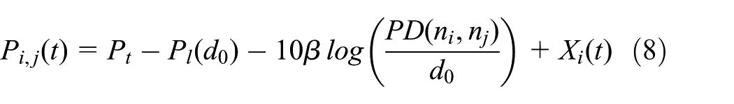
P_{i, j} (t) = P_{t} - P_{l} (d_{0}) - 10 β \log (\frac{PD (n_{i}, n_{j})}{d_{0}}) + X_{i} (t)

(8)

At time instance $t$ , the sensor node $s_{i}$ broadcasts radio signals with transmit power $P_{t}$ . During a short reference distance $d_{0}$ , the transmit power will fade due to pass loss $P_{l} (d_{0})$ , pass loss exponent $β$ and the physical distance $PD (s_{i}, s_{j})$ . Furthermore, a random noise $X_{i} (t)$ is taken into consideration. The above factors finally form the sensing result $P_{i, j} (t)$ receiving by node $s_{j}$ .

Distance correlation

For either traditional hop-based distance or SSD, the correlation coefficient between their values and physical distances is a significant index to judge the validity of regarding them as relative distance.

Figure 9 illustrates the distance correlations among hop-count, SSD, and physical distance, and correlation coefficient $ρ$ is used to quantify the relationship between two kinds of distances. As for one-hop node pairs, hop-count always remains the identical value “1” corresponding to varied physical distances (Figure 9(a), while SSD increases approximately linearly along as the actual distances increase (Figure 9(b)). Consequently, $ρ$ is 0 and 0.90, respectively. Thus, SSD can provide a sub-hop resolution which is unobtainable by hop-based approaches. The traditional hop-based distance between any two neighbors is always 1. However, the real distance between two neighbors maybe vary from 0 to their communication radius. Different from fixed hop-based distance, SSD values are variable and have high correlation with the real distance. Namely, SSD have quantized the one-hop distance. This is so-called sub-hop resolution.

Figure 9.

Distance correlation comparison: hop versus SSD: (a) hops versus distances within 1-hop, (b) SSD versus distances within 1-hop, (c) hops versus distances among multi-hops, and (d) SSD versus distances among multi-hops.

Figure 9(c) and (d) plots all the node pairs (including one-hop and multi-hop node pairs) with their hop distance, SSD, and physical distance. Figure 9(c) represents that there are only discrete integer hop distances among node pairs. Figure 9(d), meanwhile, indicates that physical distances can be mapped to continuous values, which may nicely avoid the ambiguity problem in the following localization process. Furthermore, these values of correlation coefficients verify the effectiveness of taking SSD as relative distance rather than hop-based distance.

Localization performance

The effectiveness of our design is evaluated by comparing the localization graphs and the localization errors with other three classical localization schemes. We use the terminology “DV-Hop” and “multidimensional scaling-hop (MDS-Hop)” for the original hop-based approaches, “multidimensional scaling-regulated signature distance (MDS-RSD)” for corresponding MDS method where the relative distance turns to RSD instead of shortest path hops, and “multidimensional scaling-signal based signature distance (MDS-SSD)” for the newly designed method. Special note is that in the simulations, errors are defined as offsets of Euclidean distances between expected nodes coordinates and real nodes coordinates.

Let us first look at these four localization graphs from Figure 10. Under the default configuration parameters, Figure 10 plots the localization results of our method “MDS-SSD” and other three compared algorithms. In all sub-figures, the line segments are plotted starting from nodes real positions, and pointing to the corresponding estimated positions. These four sub-figures can be treated as two groups. Namely, localization methods are driven from hop-count distance (DV-Hop and MDS-Hop) and relative distance (MDS-RSD and MDS-SSD).

Figure 10.

Localization results of four algorithms: (a) DV-Hop, (b) MDS-Hop, (c) MDS-RSD, and (d) MDS-SSD.

It is obvious that for two approaches based on hop-count distance, there are many more long black line segments than other two methods. In addition, many nodes are located to identical estimated positions, which means discrete integer mapping of hop distances mentioned by last subsection can really lead to clustering mapping in localization process. On the contrary, as shown in Figure 10(c) and (d), the latter two methods effectively reduce the ambiguity problems because that continuous mapping of relative distances may capture tiny distinction of distances with the same one-hop. The results confirm that relative distances can offer a unique sub-hop resolution while hop distances cannot. In addition, all error statistics of above four sub-figures are listed in Table 3. It can be observed that MDS-SSD achieves better localization accuracy than other three methods. Specially, MDS-SSD shows slight superiority than MDS-RSD, which owes to the combination idea of RSS comparison and RSS difference, while RSD only takes the former factor as consideration.

Table 3.

Localization errors of four algorithms (in feet).

	DV-Hop	MDS-Hop	MDS-RSD	MDS-SSD
Max error	153.15	81.82	57.85	55.88
Min error	1.63	3.11	2.25	0.32
Mean error	38.44	25.75	22.31	17.28

DV-Hop : distance vector-hop.

For the purpose to eliminate the possible bias caused by anchor selection, we increase the number of anchors from 4 to 10 in step of 1 for the network in Figure 8, whereas other system configurations remain invariant. All the statistics reported are averaged over 500 runs, and each run picks anchor nodes randomly. Figure 11(a)–(c) shows the maximum, minimum, and mean errors, respectively. As expected, the localization errors decrease with the increasing of anchor numbers for all methods. From Figure 11, we can give three remarks:

Two dashed curves are lower than two solid curves, meaning that relative distances rather than hop distances can help improve the localization accuracy. Just as mentioned above, hop distances are mapped to discrete integers, which enlarges the deviation in localization.

The novel introduced SSD method shows the best localization performance as the errors are smallest among three sub-figures.

SSD method achieves approximately 61%, 37%, and 29% performance gain by average compared with DV-Hop, MDS-Hop, and MDS-RSD, respectively.

Figure 11.

Localization errors with different numbers of anchors: (a) maximum error, (b) minimum error, and (c) mean error.

Experiments

In this section, we conduct two types of outdoor test-bed experiments: a linear network and a grid network, respectively, with 25 sensor nodes.²⁹

Experiment I: linear network

Experiment setup

Figure 12 includes a sketch map of experiment scene of the linear network and a partial in-field view. There are 25 motes deployed with the whole length of 420 ft on a side of playground, and each node is apart about 16 ft from next one.

Figure 12.

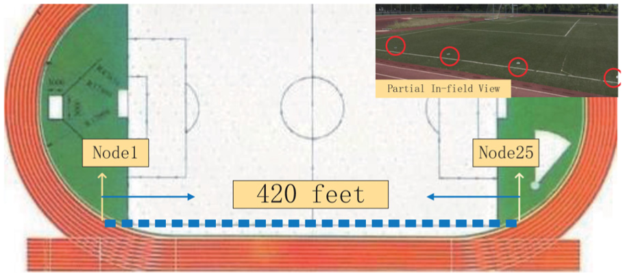
Diagrammatic sketch of experiment I: linear network.

Every node in this experiment broadcasts 100 sets of packets to the entire sensor network at the sending power of 0 dBm. After receiving several packets containing the information of node ID, RSS values and identifiers of the packets from other sensor nodes will be stored. The receiving nodes will store them in flash memory and upload them to the data platform when broadcasting has accomplished. We collect the RSS values from all the nodes and process them in the MATLAB.

In our experiments, the threshold of RSS value is regarded as −100 dBm. Namely, if the RSS value in the received packet is less than −100 dBm, the two nodes (the sender and the receiver) are considered to be non-connected and the packet can be decoded incorrectly. In other words, if the RSS value in the received packet is greater than −100 dBm, the two nodes are considered as a neighboring node pair, and then relative distance between them can be quantified through the proposed metric.

Localization performance

With four randomly picked anchors, Figure 13 shows the localization results from MDS-Hop and MDS-SSD in linear network. The dots depict sensor nodes’ real positions, and the segments are pointed to their corresponding estimated positions from real ones. Obviously, MDS-SSD has better localization performance than MDS-Hop as the segments in Figure 13(b) are much shorter than that in Figure 13(a). However, considering the singularity issues in matrix decomposition,²⁶ it is not difficult to understand that MDS-Hop is not stable for linear or close-to-linear networks. In addition, hop-based distances may cause ambiguity problems in MDS-Hop while MDS-SSD can reduce that as far as possible.

Figure 13.

Localization results of (a) MDS-Hop and (b) MDS-SSD methods.

Experiment II: grid network

Experiment setup

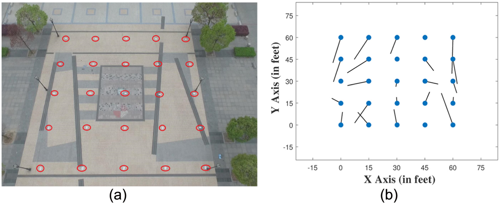
Figure 14(a) shows the outdoor experiment scenario with 25 sensor nodes. They are deployed in a $5 \times 5$ grid shape, covering an area of 60 × 60 ft². The distance between each row and column is about 15 ft. Every node broadcasts 100 packets with carrier-sensing, which consist of the sender’s node ID and a sequence number of the packet.

Figure 14.

Experiment: regular 2D network: (a) node deployment and (b) localization graph.

Localization performance

Figure 14(b) displays the localization result from the experiment with four randomly selected anchors in the network. The blue dots record the real locations of all nodes, and the black line segments are directing to the estimated positions. From the collected data, we can obtain that the localization error is about 7.9 ft averagely.

Conclusion

This article first introduces a new metric for relative distance estimation by comparing their RSS values. According to the remark from triangle cosine theorem, a novel integral approach is applied to replacing the accumulate relative distance, which finally forms SSD. Second, we describe the specific process of node localization based on MDS method. Extensive simulations and outdoor experiment are carried out to evaluate the system effectiveness from several aspects. And the results demonstrate that SSD helps improve the localization accuracy.

Footnotes

Handling Editor: Suparna De

Declaration of conflicting interests

The author(s) declared no potential conflicts of interest with respect to the research, authorship, and/or publication of this article.

Funding

The author(s) disclosed receipt of the following financial support for the research, authorship, and/or publication of this article: This work was supported, in part, by the Fundamental Research Funds for the Central Universities (grant no. 2017XKQY080).

References

Zhang

Gong

Chen

et al . Mobile sensing and simultaneously node localization in wireless sensor networks for human motion tracking. In: International conference on control automation robotics & vision, Singapore, 7–10 December 2010, pp.2313–2318. New York: IEEE.

Werner-Allen

Johnson

Ruiz

et al . Monitoring volcanic eruptions with a wireless sensor network. In: Proceedings of the second European workshop on wireless sensor networks, Istanbul, Turkey, 31 January–2 February 2005, pp.108–120. New York: IEEE.

Hammoudeh

. Putting the lab on the map: a wireless sensor network system for border security and surveillance. In: International conference on Internet of Things and cloud computing, Cambridge, 22–23 March 2016, p.4. New York: ACM.

Chen

Gao

et al . Modified extended Kalman filtering for tracking with insufficient and intermittent observations. Math Probl Eng 2015; 2015: 1–9.

Geetha

Sankar

Pankajavalli

. Energy efficient routing protocol for wireless sensor networks: an eco-friendly approach. In: International conference on eco-friendly computing and communication systems, Kurukshetra, India, 7–8 December 2015, pp.105–109. New York: IEEE.

Lederer

Wang

Gao

. Connectivity-based localization of large scale sensor networks with complex shape. In: INFOCOM 2008: the conference on computer communication, Phoenix, AZ, 13–18 April 2008, pp.789–797. New York: IEEE.

Sretenovic

Kostic

Simic

MI.

Experimental analysis of weight-compensated weighted centroid localization algorithm based on RSSI. In: International conference on telecommunication in modern satellite, cable and broadcasting services, Niš, 14–17 October 2015, pp.373–376. New York: IEEE.

Yang

Zhou

Liu

From RSSI to CSI: indoor localization via channel response. ACM Comput Surv 2013; 46: 25.

Rao

Zhu

. An advanced distributed MDS-MAP algorithm for WSNs. In: International conference on E-business and information system security, Wuhan, China, 23–24 May 2009, pp.1–5. New York: IEEE.

10.

Chowdhury

TJS

Elkin

Devabhaktuni

et al . Advances on localization techniques for wireless sensor networks: a survey. Comput Netw 2016; 110: 284–305.

11.

Shen

Zetik

Yan

et al . Time of arrival estimation for range-based localization in UWB sensor networks. In: IEEE international conference on ultra-wideband, Nanjing, China, 20–23 September 2010, pp.1–4. New York: IEEE.

12.

Chaurasia

Payal

. Analysis of range-based localization schemes in wireless sensor networks: a statistical approach. In: International conference on advanced communication technology, Gangwon-Do, Korea, 13–16 February 2011, pp.190–195. New York: IEEE.

13.

Niculescu

Nath

DV based positioning in ad hoc networks. Telecommun Syst 2003; 22(1–4): 267–280.

14.

Zhao

Pei

Zhanqi

XU.

APIT localization algorithms for wireless sensor networks. Comput Eng 2007; 45(2): 1855–1858.

15.

Niu

Huan

Chen

NMCT: a novel Monte Carlo-based tracking algorithm using potential proximity information. Int J Distrib Sens N 2016; 2016: 1–10.

16.

Xiao

et al . CSI-based indoor localization. IEEE T Parall Distr 2013; 24(7): 1300–1309.

17.

Zhang

Guo

Cui

et al . Indoor positioning optimization techniques based on RSSI. Comput Eng Appl 2015; 51(3): 235–238.

18.

Guvenc

Chong

CC.

A survey on TOA based wireless localization and NLOS mitigation techniques. IEEE Commun Surv Tut 2009; 11(3): 107–124.

19.

Liang

Zhang

Zhao

et al . TDoA for passive localization: underwater versus terrestrial environment. IEEE T Parall Distr 2013; 24(10): 2100–2108.

20.

Chen

CS.

Hybrid TOA/AOA geometrical positioning schemes using linear lines of position for mobile location. IEICE T Fund Electr 2015; E98.A(8): 1676–1679.

21.

Yang

Kong

Dai

An improved weighted centroid location algorithm. J Xian Jiaotong Univ 2010; 44(8): 1–4.

22.

Zhou

Xia

An improved APIT node self-localization algorithm in WSN. In: World congress on intelligent control and automation (WCICA 2008), Chongqing, China, 25–27 June 2008, pp.7582–7586. New York: IEEE.

23.

Zhang

et al . A novel node localization algorithm for anisotropic wireless sensor networks with holes based on MDS-MAP and EKF. In: 2016 IEEE region 10 conference (TENCON), Singapore, 22–25 November 2016, pp.3022–3025. New York: IEEE.

24.

Mariakakis

Sen

Lee

et al . SAIL: single access point-based indoor localization. In: Proceedings of the 12th annual international conference on mobile systems, applications, and services, Bretton Woods, NH, 16–19 June 2014, pp.315–328. New York: ACM.

25.

Yang

Chen

et al . Tagoram: real-time tracking of mobile RFID tags to high precision using COTS devices. In: Proceedings of the 20th annual international conference on mobile computing and networking, Maui, HI, 7–11 September 2014. New York: ACM.

26.

Zhong

RSD: a metric for achieving range-free localization beyond connectivity. IEEE T Parall Distr 2011; 22(11): 1943–1951.

27.

Wang

et al . View recognition based on Procrustes shape analysis for gait identification. In: Chinese control conference, Nanjing, China, 28–30 July 2014. New York: IEEE.

28.

Fall

Varadhan

(eds). Radio propagation models. In: The ns manual (formerly ns notes and documentation): VINT Project, 2005, https://www.scribd.com/document/54645310/Ns-Manual-Ns-Doc

29.

Ahmed

Bouk

Javaid

et al . RF propagation analysis of MICAz Mote’s antenna with ground effect. In: Multitopic conference, Islamabad, Pakistan, 13–15 December 2012, pp.270–274. New York: IEEE.

Localization with signal-based signature distance

Abstract

Keywords

Introduction

Related work

Motivation

System design

Relative distance quantization

Sequential distance estimation

Definition 1

Signal-based signature distance estimation

Definition 2

SSD integral calculation

Physical coordinate generation

Relative map construction

Procrustes analysis

Simulation

Simulation configurations

Distance correlation

Localization performance

Experiments

Experiment I: linear network

Experiment setup

Localization performance

Experiment II: grid network

Experiment setup

Localization performance

Conclusion

Footnotes

Declaration of conflicting interests

Funding

References