Sage Journals: Discover world-class research

Abstract

Localization is one of the essential issues in wireless sensor networks. Randomly deployed sensor nodes that do not own any positioning device need to determine their locations for further purposes. Range-based schemes typically utilize extra hardware to provide higher accuracy based on either node-to-node distances or angles. On the other hand, range-free mechanisms support coarse localization without the specific equipment. The paper presents a range-free localization scheme with aerial anchor nodes. Each aerial anchor flies across the sensing field and also periodically broadcasts its location information obtained from its GPS receiver. The sensor nodes use the information and geometry principles to calculate their positions. With the mechanism, the sensor nodes do not need distance-probing hardware or additional communication among them. The localization mechanism has been evaluated and the results show that the mechanism had better performance than other range-free mechanisms.

Keywords

Wireless Sensor Networks Localization Range-Free Mobile Beacons Aerial Anchors Geometry

1. Introduction

Wireless sensor networks have been highlighted in recent years [1]. A sensor network consists of a large number of sensor nodes that are randomly deployed in a sensing field. A sink node is responsible for receiving instructions from a commander for assigning tasks to all sensor nodes. If the sensor nodes are aware of the occurrence of the events, they will deliver the collected information to the sink node. The sink node thus gathers all needed data and notifies the commander of the result. With ad hoc transmission technology, each sensor node can communicate directly with others in its neighborhood [2]. For connecting with nodes which are out of the radio range, the sensor nodes use multi-hop routing for data transmission.

Localization is a fundamental issue in wireless sensor networks [3]. Location information can be exploited for routing, coverage, deployment, tracking, and other location-dependent applications. For example, location-dependent routing protocols utilize location information to reduce route discovery overhead and power consumption [4]. Several mechanisms have been proposed for sensor localization. These schemes can be classified into two styles: range-based and range-free. The range-based approach needs to acquire distance or angle information for performing triangulation (lateration or angulation) for localization [5 –11]. The information can be obtained based on Time of Arrival (TOA), Time Difference of Arrival (TDOA), Angle of Arrival (AOA), and Received Signal Strength Indicator (RSSI) technologies [12 –14]. Although the range-based methods were fairly accurate (less than two meters [8, 11]), each sensor node must carry special and expensive hardware. The range-free approach uses proximity or hop-count techniques to explore locations of sensor nodes without distance or angle information [15 –19]. The approach typically needs lots of beacon nodes, specifically arranged deployments, or interactions among neighboring sensor nodes for improving accuracy. The best case in location error was about 10% of the radio range [17].

This paper describes a range-free localization mechanism with mobile aerial anchors in the sensor network. Our localization method is based on the geometry corollary that states a perpendicular line coming through the center of a sphere's circular cross section (a circle) passes through the center of the sphere (See Appendix). Consider that the communication range of a sensor node is an approximate sphere and the sensor node is located at the center of the sphere. The aerial anchor nodes flying over the sensing field broadcast their current positions. Each sensor node selects the appropriate information transmitted by the anchor nodes for forming a circular cross section of the sphere. Therefore, the center of the sphere (the sensor node's location) can be estimated by resolving the intersection point of the perpendicular line and the ground. The localization scheme eliminates the power consumption for communication among sensor nodes because only aerial anchors are required to broadcast beacon messages. More improvements, such as jittered beacon scheduling, chord selection, and circular cross-section selection, are developed for enhancing the localization performance. The aerial anchors provide one more dimensional mobility so our mechanism is less affected by geographical limitations (such as rivers, lakes, and obstacles) compared to the schemes using ground anchors [21 –25].

The mechanism has been evaluated with the network simulator ns-2. The simulation results show that our scheme determined positions of sensor nodes precisely and outperformed previous range-free methods. The location accuracy was also competitive to other range-based approaches [3,8,11]. Both the execution time and the number of beacon messages were reduced in our mechanism.

2. Related Work

2.1 Mobile Beacons

Sichitiu and Ramadurai described a localization mechanism using a single mobile beacon for transmitting its current position [21]. A sensor node receiving the beacon can recognize that it is in the area around the mobile beacon. Combined with the RSSI technique, possible locations of the sensor node can be estimated. Dutta and Bergbreiter measured the distance from a sensor node to a mobile object based on ultrasound technology [22]. Neighboring sensor nodes cooperated to determine their locations using the range-based approach. Sun and Guo proposed probabilistic localization schemes with a mobile beacon [23]. The schemes used the TOA technique for ranging and utilized the centroid formula with distance information to calculate a sensor node's position. Galstyan et al. lowered the uncertainty of positions for sensor nodes based on radio connectivity constraints [24]. With each received beacon, the receiver's location is bounded in the transmission area of the sender. Our previous research utilized mobile anchor points for range-free localization [25].

2.2 Flying Robots

Corke et al. developed a flying robot navigation application in a sensor network [26, 27]. The flying robot participated in the localization process by broadcasting its current position. The work indicated that the constraint scheme [24] provided higher accuracy than other mechanisms, including strongest signal, mean, and median schemes.

3. Aerial Anchor Nodes

3.1 System Environments and Assumptions

The system environment consists of a group of sensor nodes on the ground and aerial anchor nodes as illustrated in Fig. 1. The sensor nodes are randomly distributed in the sensing field. Each sensor node performs its sensing task based on the applications. The mobile aerial nodes are able to fly above the sensing filed for supporting sensor nodes to determine their positions.

Figure 1

Example of system environment.

There are some main assumptions in the localization mechanism. First, each aerial anchor node equips with a Global Positioning System (GPS) receiver. Next, the aerial anchors have sufficient energy for flying and communication during the localization process. Last, the aerial anchors can fly by themselves or other carriers such as helicopters.

3.2 Localization Scheme

The localization scheme is based on the geometric corollary in which a perpendicular line that comes through the center of a sphere's circular cross section passes through the center of the sphere. Fig. 2 shows that a perpendicular line (L) passes through both the center of the circular cross section (C) and the center of the sphere (S). The intersection point of L and the plane XY is S. Therefore, the localization problem can be transformed based on the corollary. The center of the sphere is the location of the sensor node; the radius of the sphere is the largest distance where the sensor node can communicate with the aerial anchor node.

Figure 2

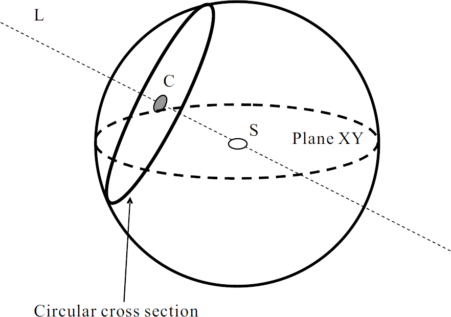
The circular cross section of a sphere.

3.2.1 Beacon Point Selection

The localization process includes two phases. The first phase calculates the center of the circular cross section (circle). The second phase computes the intersection point of the perpendicular line that passes through the circular cross section's center and the ground. With our mechanism, at least three endpoints on the sphere should be gathered to construct a circular cross section. The endpoint on the sphere is the position where the aerial anchor node passes through the sphere. Each anchor node periodically broadcasts beacon messages during moving. The beacon's identification, location, and timestamp are included in the beacon message. Each sensor node maintains a set of beacon points and a Visitor List. The beacon point is regarded as an approximate endpoint on the sensor node's communication sphere. The Visitor List records both identifications and corresponding lifetime of the aerial anchors whose messages have been obtained by the sensor node. The i-th beacon point of the sensor node is represented as (id_i, location_i) and the j-th entry in the Visitor List is logged as (id_j, location_j, lifetime_j). The lifetime of an aerial anchor is used for verifying the sensor node is within the radio range of the aerial anchor or not. When a sensor node receives a beacon message from the aerial anchor node, the sensor node will check whether the aerial node is in its Visitor List or not. If not, a beacon point will be recorded and the aerial node's identification with its predefined lifetime will also be inserted in the Visitor List. Otherwise, the beacon message will be discarded and the lifetime of the aerial node will be prolonged. When the lifetime of the aerial anchor is expired, the last beacon message of the aerial node will be regarded as a beacon point and the corresponding entry for the anchor in the Visitor List will be removed. The detailed algorithm for the beacon point selection is presented in Fig. 3

Figure 3

Beacon point selection algorithm.

An example for the beacon point selection is illustrated in Fig. 4. An anchor node (A) moves from (x, y, z) to (x′, y′, z′) and broadcasts beacon messages with an interval t where t = T_i₊₁ − T_i, i = 0, …, 7. With the selection principle, the beacon message at T₂ is considered as a beacon point (A, (x₂, y₂, z₂)) for the sensor node (S). Node S adds an entry (A, (x₂, y₂, z₂), T₂ + δ) in its Visitor List. The δ is the predefined lifetime for aerial nodes and the value of δ should be larger than the beacon interval t (δ= αt, α> 1). The lifetime of node A is increased by δ at T₃, T₄, T₅, and T₆. After node A leaves the communication sphere of node S and node A's lifetime expires, node A's beacon message at T₆ will be chosen as a beacon point and node S will delete the entry for node A in its Visitor List.

Figure 4

Beacon point selection.

3.2.2 Location Calculation

After the circular cross section is established, the perpendicular line (L) that passes through the center of the circular cross section can be determined. Consider a set of selected beacon points {B_i, B_j, B_k} with their corresponding locations (x_i, y_i, z_i), (x_j, y_j, z_j), and (x_k, y_k, z_k) in Fig. 5. The normal vector and the center of the circular cross section are required for forming the perpendicular line. The normal vector of the circular cross section (N) can be solved by the cross product of $\vec{B_{j}} B_{k}$

\vec{N} = \vec{B_{i}} B_{j} \times \vec{B_{j}} B_{k} = (N_{x}, N_{y}, N_{z})

(1)

Figure 5

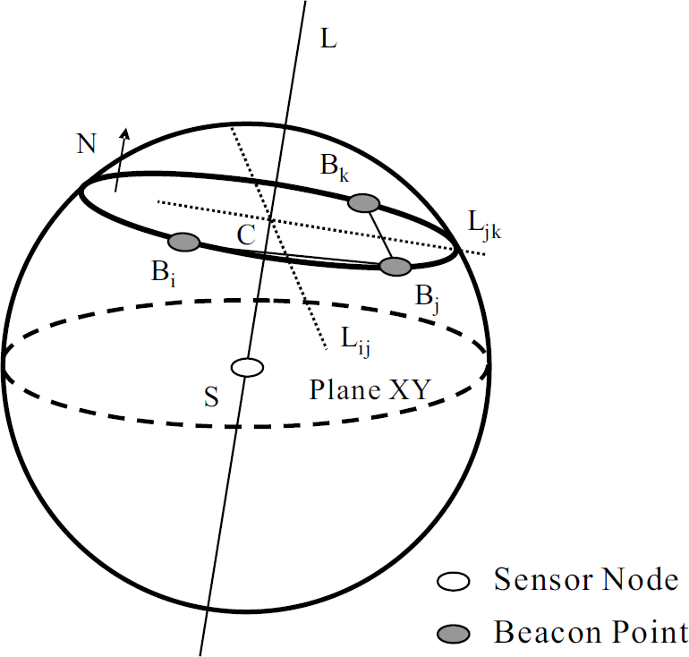
Location calculation.

Based on the corollary in which the perpendicular bisector of any chord passes through the center of the circle [20], the intersection point of the perpendicular bisectors of two chords in the same circle is the center of the circle. With perpendicular principle, the perpendicular bisector L_ij can be generated by the cross product of $\vec{N}$ and $\vec{B_{i}} B_{j}$ . Similarly, the cross product of $\vec{N}$ and $\vec{B_{j}} B_{k}$ is the perpendicular bisector L_jk.

According to the corollary, the intersection point of two lines L_ij and L_jk is the center of the circle C located at (x_c, y_c, z_c).

The equation of the perpendicular line L can be donated as

L : \frac{x - x_{c}}{N_{x}} = \frac{y - y_{c}}{N_{y}} = \frac{z - z_{c}}{N_{z}} = t .

(2)

The center of the sphere can be obtained by solving the intersection point of the L and plane XY. The estimated location of the sensor node is shown as

{\begin{cases} x_{s} = N_{x} * t + x_{c}, \\ y_{s} = N_{y} * t + y_{c}, \\ z_{s} = N_{z} * t + z_{c}, where t = - (\frac{z_{c}}{N_{z}}) . \end{cases}

(3)

Enhancements

4.1 Beacon Scheduling

Broadcasting may introduce problems, such as destructive congestion, contention, and collision, and thus affects performance for the wireless ad hoc networks [28]. The collision at sensor nodes could also occur in our mechanism. The scheduling for broadcasting beacon messages is jittered for dealing with the problem. The jitter time is randomly selected from a uniform distribution between 0 and (0.01 ∗ beacon interval). The jittered beacon interval is shown as follows.

Jittered beacon interval = beacon interval + jitter time

(4)

The sensor nodes can efficiently obtain beacon messages from different aerial nodes because the jittered scheduling reduces the beacon collision at the sensor nodes. The detailed performance for jitters has been analyzed [29].

4.2 Chord Selection

If the selected beacon points are exactly on the communication sphere, the localization will perform accurately. However, in practical environments, it is possible to collect incorrect beacon points because of collision or inappropriate beacon intervals. The chords constructed by the erroneous beacon points cannot locate the center of a circular cross section successfully. With a bird's eye view on the circular cross section, Fig. 6 demonstrates faulty localization error due to the improper chords. Based on our observations, the probability of failed localization will be higher when the short chord appears. A threshold (λ) for the length of a chord is used to avoid short chords. The relationship between the threshold and the communication sphere's radius (R) is

0 < λ \leq 2 R .

(5)

Figure 6

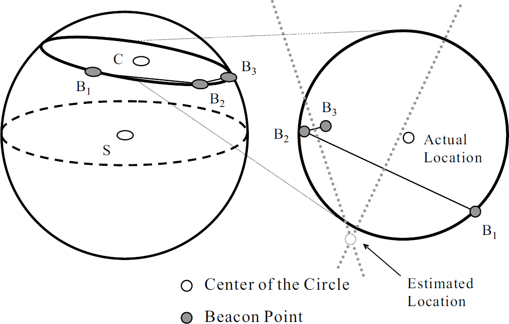
Chord selection.

Based on our observations, the length of a chord must exceed a threshold for decreasing the localization error. Appropriate values for the threshold λ will be investigated in Section 5.

4.3 Circular Cross Section Selection

In addition to chord selection, choosing an appropriate circular cross section can improve the localization accuracy. In our study, when the included angle Θ between the normal vectors of the circular cross section ( $\vec{N}$ ) and the ground ( $\vec{Z}$ ) is closer to 90 degrees, the mechanism has higher possibility of failing to locate the positions of sensor nodes. The cos Θ can be computed as

cos Θ = \frac{\vec{N} \cdot \vec{Z}}{| \vec{N} | | \vec{Z} |} .

(6)

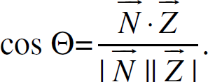
As depicted in Fig. 7, the large localization error occurs when the circular cross section and the ground are approaching to perpendicular. For coping with the issue, setting a threshold (μ) to limit the included angle is required. The Θ must not exceed μ degrees where 0 ≤ μ < 90. The relation between the location error and the threshold μ for the included angle will be discussed in Section 5.

Figure 7

Circular cross section selection.

5. Performance Evaluations

Our simulations were implemented based on the ns-2 network simulator with the Monarch Project wireless and mobile extensions [30, 31]. The Lucent WaveLAN IEEE 802.11 product with 2 Mbps bandwidth was used for the radio model and its Distributed Coordination Function (DCF) was utilized for Medium Access Control (MAC) model. Other MAC protocols with sleep/wake-up modes (e.g., S-MAC [32]) can be used with our mechanism as well. Each sensor node is required to stay in a wake-up mode during the localization process. After the sensor node obtains its location, it can enter the sleep mode for saving power.

5.1 Environment

The wireless extensions of the ns-2 network simulator did not support three-dimensional environments so some modifications were made for our simulations. The changes included

extending the boundary of the simulated environment to the three-dimensional space (X, Y, and Z coordinates),

modifying the radio propagation model, and

stretching out the movement models for mobile aerial anchors.

The sensing field was 100 ∗ 100 m² in the simulations. There were 300 randomly deployed sensor nodes in the area. Each aerial anchor was randomly placed in the corners of the simulated area at the beginning as shown in Fig. 8. The aerial anchors cannot be arranged within the sensing field initially, or the sensor node will take the first beacon message as a beacon point that is not located on the communication sphere. The transmission range of the aerial anchors was R. Assume that each anchor node was carried by a remote-controlled helicopter. The aerial anchors flied in the movement space with (100 + 2R) ∗ 100 ∗ R m³. The three-dimensional movement model for aerial anchors was derived from Random Waypoint model [33]. Each aerial anchor selected a random destination within the movement space and then flied to the location with a constant speed. When the aerial anchor arrived at the destined position, the anchor journeyed to the next destination without pause time. The aerial anchors keep moving in the movement space based on the movement model for broadcasting beacon messages. The simulation was terminated when all sensor nodes obtained their locations.

Figure 8

Simulation environment.

5.2 Simulation Settings

Table I displays the detailed parameter settings for our simulations. The default values used during the simulations were within the parentheses. Centroid [15] and Constraint [24], both well-known range-free localization schemes, were implemented for performance comparison. The Centroid mechanism was modified to utilize aerial anchors for sensor position determination. With the Centroid mechanism, each sensor node gathers beacon messages sent by aerial anchors. 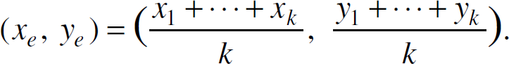After receiving k beacon messages, the sensor node calculates its location based on centroid formula that is

(x_{e}, y_{e}) = (\frac{x_{1} + \dots + x_{k}}{k}, \frac{y_{1} + \dots + y_{k}}{k}) .

(7)

Table 1

Simulation Parameters

Parameter	Value(s)
Beacon interval	(0.1), 0.3, 0.5, 0.7, 0.9 sec
Visitor list lifetime	(3 * beacon interval)
Beacon scheduling	(jittered), periodical
Threshold for chords	0%, 10%, 20%, 30%, (40%), 50% of R
Threshold for included angles	90, 88, 86, 84, (82), 80 degrees
Moving speed	(10), 20, 30, 40, 50 m/sec
Radio range	10, 15, (20), 25 m
# of aerial anchors	1%, (2%), 3%, 4%, 5% of sensor nodes

Constraint scheme considers that the uncertainty in a sensor node's location is a rectangular region $Q_{i} = [x_{i}^{m i n}, x_{i}^{m a x}] \times [y_{i}^{m i n}, y_{i}^{m a x}]$ . The initial region of each sensor node is the size of the sensing field (e.g., Q₀ = [0, L] × [0, L]). When the sensor node receives a beacon message (x_b, y_b), the node will update its rectangular region for lessening the uncertainty of its position based on following rule: Q_i = Q_i−1 ∩ [x_b − r, x_b + r] × [y_b − r, y_b + r], where r is radio range of the aerial anchor. After detecting k beacon messages, the estimated position of the sensor node is the centroid of the rectangle. Based on our simulation, the average location error for both Centroid and Constraint schemes converged after each sensor node received at least k = 200 beacon messages (see Fig. 9).

Eight sets of simulations are described as follows.

Beacon scheduling: The evaluation compared the localization accuracy between the jittered scheduling and periodical scheduling. Each simulation utilized five different beacon intervals.

Threshold for the length of a chord: There were six varying thresholds. The simulation can verify suitable thresholds for the length of chords with the localization mechanism.

Threshold for the included angle between normal vectors of the circular cross section and the ground: The simulation sets six thresholds for the included angle. The appropriate included angle can be discovered for promoting localization accuracy.

Radio range: The evaluation was for analyzing three localization schemes with four different radio ranges.

Moving speed: The simulation studied the impact of moving speeds on three mechanisms.

Number of aerial anchors: Three approaches were compared using varying numbers of aerial anchor nodes.

Figure 9

Accuracy convergence for Centroid and Constraint.

Three metrics were used to evaluate the performance for the localization mechanisms:

Average location error: the average distance between the estimated location (Xe_i, Ye_i, Ze_i) and the actual location (X_i, Y_i, Z_i) of all sensor nodes.

Average location error = \frac{\sum \sqrt{(X e_{i} - X_{i})^{2} + (Y e_{i} - Y_{i})^{2} + (Z e_{i} - Z_{i})^{2}}}{# o f s e n s o r n o d e s}

(8)

Average execution time: The average execution time for the sensor nodes to acquire their locations. The execution time (localization time) for a sensor node is calculated from the starting of the simulation to the determination of the sensor node's position.

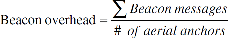
Average execution time = \frac{\sum E x e c u t i o n_t i m e_{i}}{# o f s e n s o r n o d e s}

(9)

Beacon overhead: the average number of beacon messages broadcast by the aerial anchors until the simulation was terminated.

Beacon overhead = \frac{\sum B e a c o n m e s s a g e s}{# o f a e r i a l a n c h o r s}

(10)

5.3 Results

5.3.1 Beacon Scheduling

As displayed in Fig. 10, decreasing the beacon interval reduced the localization error for both the jittered and the periodical beacon scheduling mechanisms. The location error of the periodical scheme with all intervals was about 14 meters. The beacon collision problem was more serious as the beacon interval decreased. Therefore, the improvement by broadcasting more beacons in the periodical scheme was little. Contrary to the periodical scheme, the localization accuracy was advanced to about 0.8 meter in the jittered scheduling when the beacon interval was set to 0.1 second. The results show that the jittered beacons ameliorated the localization accuracy by improving the collision problem. The required execution time for localization process was also lessened by reducing beacon collision at each sensor node (see Fig. 11). Compared to the periodical scheme, the jittered scheduling approach improved at least 200 seconds in average execution time. Communication overhead in our mechanism only included broadcast beacon messages. In Fig. 12, the beacon overhead for both schemes enlarged as the beacon interval was reduced. The periodical scheme required more beacon messages than the jittered approach. When the beacon interval was 0.1 second, the difference in the number of beacons between two methods was about 6500.

Figure 10

Average location error vs. beacon scheduling.

Figure 11

Average execution time vs. beacon scheduling.

Figure 12

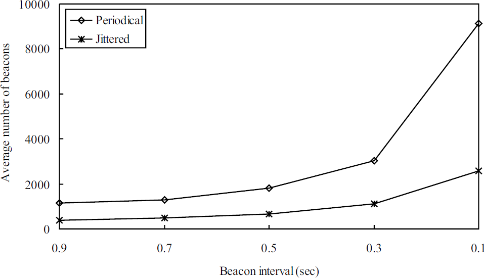
Beacon overhead vs. beacon scheduling.

5.3.2 Chord Selection

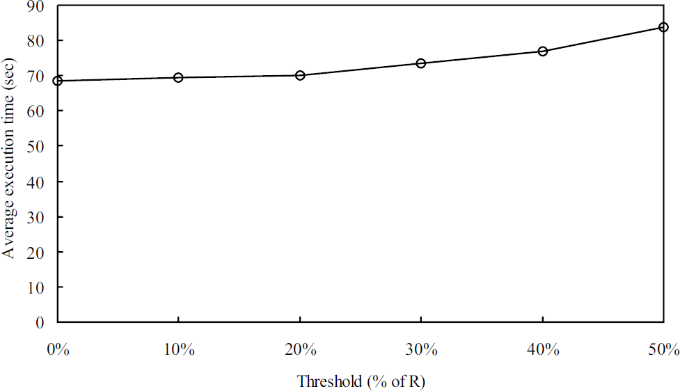
The simulation examined five varying thresholds for the length of chords from 0% to 50% of radio range. The length of all chords had to surpass the threshold. The 0% represents no limitation for the length of a chord. Fig. 13 demonstrates that the chord selection mechanism dramatically enhanced the localization performance for our approach. When the threshold was increased to 50% of radio range, the location error was improved further to about 0.7 meter.

Figure 13

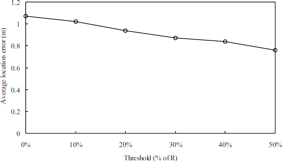
Average location error vs. threshold for the length of a chord.

As shown in Fig. 14 and Fig. 15, the average execution time and beacon overhead increased slightly following the growth of the threshold. The sensor nodes spent more time on gathering valid chords so more beacon messages were broadcast by the aerial anchor nodes. According to the results, the appropriate threshold was about 40% of the radio range so the value was set as the default threshold for the following simulations.

Figure 14

Average execution time vs. threshold for the length of a chord.

Figure 15

Beacon overhead vs. threshold for the length of a chord.

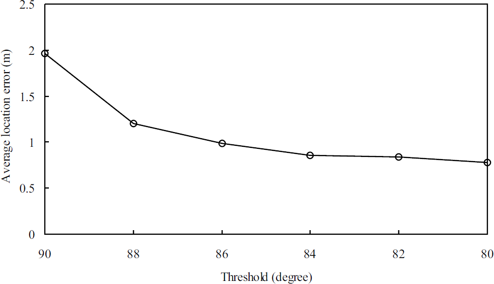
5.3.3 Circular Cross Section Selection

With default simulation settings, Fig. 16 depicts the location errors and the included angles for all sensor nodes. All huge location errors occurred apparently when the included angles were approaching to 90 degrees. The improper circular cross sections harmed the localization accuracy significantly. The threshold for the included angles between normal vectors of the circular cross section and the ground was set from 90 to 80 degrees. The included angle had to be smaller than the threshold. The 90 degrees mean that any included angle was valid. The results indicate that arranging the threshold for the included angle did help the accuracy (see Fig. 17). The location error fell down rapidly from 1.9 to 0.7 meter due to the smaller thresholds. Fig. 18 and Fig. 19 show that the needed additional execution time and beacon overhead were limited. When the threshold was set to 80 degrees, only 1% extra execution time and 4% additional beacon messages were required. Based on the results, the default value for the included angle threshold was set to 82 degrees in the remaining simulations.

Figure 16

Location error vs. included angle.

Figure 17

Average location error vs. threshold for the included angle.

Figure 18

Average execution time vs. threshold for the included angle.

Figure 19

Beacon overhead vs. threshold for the included angle.

5.3.4 Radio Range

Fig. 20 compares the performance for Centroid, Constraint, and our scheme with four different radio ranges. The location errors of Centroid and Constraint schemes were increased with the larger transmission ranges. Concerning the percentage of radio ranges, the accuracy for Centroid and Constraint were remained about 15% and 10% of the radio range, respectively. On the other hand, our scheme improved the localization error with longer chords. The accuracy for our mechanism was promoted from 0.8 (5% of R) to 0.6 meter (2% of R). Both Centroid and Constraint used the proximity concept to estimate sensor nodes' positions so they could not provide the same accuracy as our mechanism did.

Figure 20

Average location error vs. radio range.

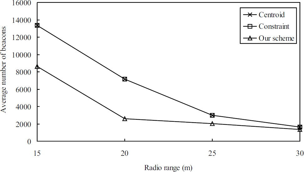
The execution time and beacon overhead for three schemes were reduced when the radio range was enlarged (see Fig. 21 and Fig. 22). With the larger ranges, the beacon messages broadcast by each aerial node were received by more sensor nodes. The sensor nodes thus required less time for localization. The numbers of the beacons were lower as well due to the shorter needed execution time. Our mechanism achieved the best performance in both execution time and beacon overhead because the sensor node only required collecting several appropriate beacon points for localization. With Centroid or Constraint method, 200 beacon messages were necessary to compute the location for each sensor node as mentioned in Section 5.2. Based on the identical movement patterns of the aerial anchors and the number of received messages, the execution time and beacon overhead for both Centroid and Constraint were the same.

Figure 21

Average execution time vs. radio range.

Figure 22

Beacon overhead vs. radio range.

5.3.5 Moving Speed

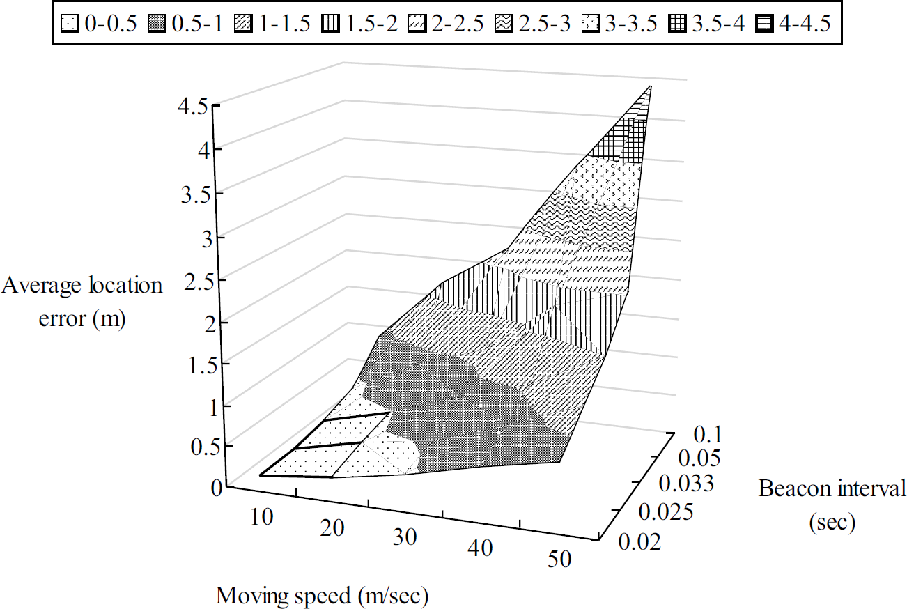
Fig. 23 depicts the relation for the location error, the moving speed, and the beacon interval of the aerial anchors. In order to conform to the accuracy level and energy concern, the corresponding moving speed and beacon interval should be selected carefully. A large beacon interval results in inaccurate localization and a small beacon interval consumes energy quickly for the aerial anchors. The simulation investigated the impact on the moving speed for three localization schemes with the accuracy level (0.5 to 1 m). The corresponding intervals based on the accuracy level were 0.1, 0.05, 0.033, 0.025, and 0.02 second for moving speed 10, 20, 30, 40, and 50 m/sec, respectively.

Figure 23

Location error vs. beacon interval and moving speed.

Fig. 24 displays that the speed of the aerial anchors did not affect the localization performance. The average location errors for Centroid, Constraint, and our scheme were remained about 3, 2, and 0.8 meter, respectively. With the faster speeds for the aerial anchors, the sensor nodes collected more beacons during the same time period so the average execution time was diminished (see Fig. 25). In Fig. 26, when the moving velocity was not above 30 m/sec, the beacon overhead increased due to the reduction of the beacon interval. However, with the speed larger than 40 m/sec, the overhead was dropped for all three mechanisms because the execution time was shortened.

Figure 24

Average location error vs. moving speed.

Figure 25

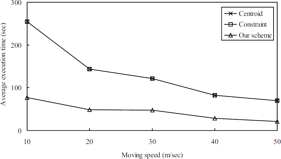
Average execution time vs. moving speed.

Figure 26

Beacon overhead vs. moving speed.

5.3.6 Number of Aerial Anchors

Our localization mechanism had the best performance in terms of the location error, the execution time, and the beacon overhead with varying numbers of aerial anchor nodes (see Fig. 27, Fig. 28, and Fig. 29). The average errors for Centroid, Constraint, and our scheme were steadily remained at 3, 2, and 0.8 meter. Our scheme located the sensor nodes' positions accurately under varying number of aerial anchors. More aerial nodes contributed to decrease the execution time because the sensor nodes gathered sufficient beacon messages more quickly. The average beacon overhead was also reduced.

Figure 27

Average location error vs. number of aerial anchors.

Figure 28

Average execution time vs. number of aerial anchors.

Figure 29

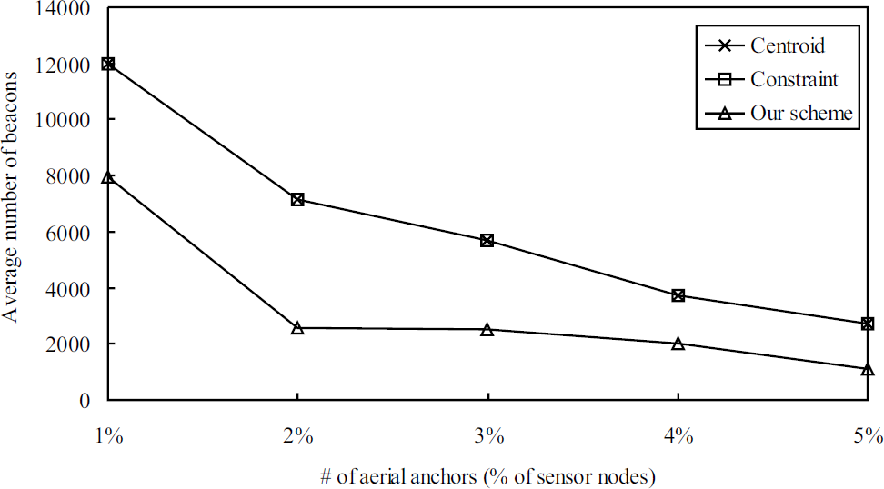
Beacon overhead vs. number of aerial anchors.

5.3.7 Error Distribution

The error distribution can reveal the precision of a localization system. Fig. 30 displays the cumulative localization error distribution for the three mechanisms. The precision of our localization scheme surpassed both Centroid and Constraint mechanisms. Our localization scheme located positions for 97% of the sensor nodes within three meters. Constraint scheme reached 82% and Centroid approach only had 50% of the sensor nodes within three meters.

Figure 30

Cumulative localization error distribution.

Conclusion

This paper demonstrated that the range-free localization mechanism was able to achieve accurate sensor position determination. Based on the location information from aerial anchors and the geometry corollary, the sensor nodes can estimate their positions precisely. All computation is performed locally without extra interactions and the beacon overhead only occurs on aerial nodes so the mechanism is distributed, scalable, effective, and power efficient. Several refinements, including chord selection, circular cross section selection, and jittered beacon scheduling, were also discussed. Increasing the moving speed, the radio range, or the number of aerial anchors can reduce needed execution time. The mechanism was successfully implemented and evaluated using ns-2. According to the simulation results, our mechanism outperformed two previous range-free localization schemes in location accuracy, execution time, and overhead.

Footnotes

Appendix

References

Akyildiz

I. F.

Sankarasubramaniam

, and Cayirci

, “A Survey on Sensor Networks,” IEEE Communications Magazine, 40, 8, 102–114, Aug., 2002.

Royer

E. M.

, and Toh

C.-K.

, “A Review of Current Routing Protocols for Ad Hoc Mobile Wireless Networks,” IEEE Personal Communications, 6, 2, 46–55, Apr., 1999.

Hightower

, and Borrielio

, “Location Systems for Ubiquitons Computing,” IEEE Computer, 34, 8, 57–66, Aug., 2001.

, and Vaidya

N. H.

, “Location Aided Routing in Mobile Ad Hoc Networks,” Proceedings of ACM International Conference on Mobile Computing and Networking (MOBICOM), 66–75, Feb., 1998.

Hightower

Boricilo

, and Want

, “SpotON: An Indoor 3D Location Sensing Technology Based on RF Signal Strength,” Tech. Rep. UW CSE, 00-02-02, University of Washington, Feb., 2000.

Bahl

, and Padmanabhan

V. N.

, “RADAR: An In-Building RF-Based User Location and Tracking System,” Proceedings of IEEE Joint Conference of the IEEE Computer and Communications Societies (INFOCOM), 775–784, Mar., 2000.

Priyantha

N. B.

Chakrnborty

, and Balakrishnan

, “The Cricket Location-Support System,” Proceedings of ACM International Conference on Mobile Computing and Networking (MOBICOM), 32–43, Aug., 2000.

Savvides

Han

C. C.

, and Srivastava

M. B.

, “Dynamic Fine-Grained Localization in Ad-Hoc Networks of Sensors,” Proceedings of ACM International Conference on Mobile Computing and Networking (MOBICOM), 66–179, July, 2001.

Niculoscu

, and Nath

, “Ad Hoc Positioning System (APS) Using AoA,” Proceedings of IEEE Joint Conference of the IEEE Computer and Communications Societies (INFOCOM), 1734–1743, Mar., 2003.

10.

Nasipuri

, and Li

, “A Directionality Based Location Discovery Scheme for Wireless Sensor Networks,” Proceedings of ACM International Workshop on Wireless Sensor Networks and Applications (WSNA), 105–111, Sept., 2002.

11.

Patwari

Hero

A. O.

Perkins

Correal

N. S.

, and O'Dea

R. J.

, “Relative Location Estimation in Wireless Sensor Networks,” IEEE Transactions on Signal Processing, 51, 8, 2137–2148, Aug., 2003.

12.

Klukas

, and Fattouche

, “Line-of-Sight Angle of Arrival Estimation in The Outdoor Multipath Environment,” IEEE Transactions on Vehicular Technology, 47, 1, 342–351, Feb., 1998.

13.

Cong

, and Zhuang

, “Hybrid TDOA/AOA Mobile User Location for Wideband CDMA Cellular Systems,” IEEE Transactions on Wireless Communications, 1, 3, 439–147, July, 2002.

14.

McGuire

Plataniotis

K. N.

, and Venetsanopoulos

A. N.

, “Location of Mobile Terminals Using Time Measurements and Survey Points,” IEEE Transactions on Vehicular Technology, 52, 4, 999–1011, July, 2003.

15.

Bulusu

Heidemann

, and Estrin

, “GPS-less Low Cost Outdoor Localization for Very Small Devices,” IEEE Personal Communications, 7, 5, 28–34, Oct., 2000.

16.

Niculescu

, and Nath

, “DV Based Positioning in Ad Hoc Networks,” Kluwer Journal of Telecommunication Systems, 22, 1, 267–280, Jan., 2003.

17.

Huang

Blum

B. M.

Stankovic

J. A.

, and Abdelzahor

, “Range-Free Localization Schemes for Large Scale Sensor Networks,” Proceedings of ACM International Conference on Mobile Computing and Networking (MOBICOM), 81–95, Sept., 2003.

18.

Liu

, and He

, “Sensor Localization with Ring Overlapping Based on Comparison of Received Signal Strength Indicator,” Proceedings of IEEE International Conference on Mobile Ad-hoc and Sensor Systems (MASS), 516–518, Oct., 2004.

19.

Stoleru

, and Stankovic

J. A.

, “Walking GPS: A Practical Solution for Localization in Manually Deployed Wireless Sensor Networks,” Proceedings of IEEE International Conference on Local Computer Networks (LCN), 480–489, Nov., 2004.

20.

Travers

K. J.

Dalton

L. C.

, and Layton

K. P.

, Geometry, Laidlaw, 1987.

21.

Sichitiu

M. L.

and Ramadurai

, “Localization of Wireless Sensor Networks with A Mobile Beacon,” Proceedings of IEEE International Conference on Mobile Ad-hoc and Sensor Systems (MASS), 174–183, Oct., 2004.

22.

Dutta

and Bergbreiter

, “MobiLoc: Mobility Enhanced Localization.” http://www.cccs.berkeley.edu/prabal/projects/cs294-1/, 2005.

23.

Sun

G.-L.

, and Guo

, “Comparison of Distributed Localization Algorithms for Sensor Network with A Mobile Beacon,” Proceedings of IEEE International Conference on Networking, Sensing and Control (ICNSC), 536–540, Mar., 2004.

24.

Galstyan

Krishnamadhari

Lerman

, and Patterm

, “Distributed Online Localization in Sensor Networks Using A Mobile Target,” Proceedings of International Symposium on Information Processing in Sensor Networks (IPSN), 61–70, Apr., 2004.

25.

Ssu

K. F.

C. H.

, and Jiau

H. C.

, “Localization with Mobile Anchor Points in Wireless Sensor Networks,” IEEE Transactions on Vehicular Technology, 54, 3, 1187–1197, May, 2005.

26.

Corke

Peterson

, and Rus

, “Networked Robots: Flying Robot Navigation Using a Sensor Net,” Proceedings of International Symposium on Robotics Research (ISRR), Oct., 2003.

27.

Corke

Peterson

, and Rus

, “Coordinating Aerial Robots and Sensor Networks for Localization and Navigation,” Proceedings of the International Symposium on Distributed Autonomous Robotic Systems (DARS), June, 2004.

28.

S.-Y.

Tseng

Y.-C.

Chen

Y.-S.

, and Sheu

J.-P.

, “The Broadcast Storm Problem in A Mobile Ad Hoc Network,” Proceedings of ACM International Conference on Mobile Computing and Networking (MOBICOM), 151–162, Aug., 1999.

29.

Williams

, and Camp

, “Comparison of Broadcasting Techniques for Mobile Ad Hoc Networks,” Proceedings of ACM International Symposium on Mobile Ad Hoc Networking and Computing (MOBIHOC), 194–205, June, 2002.

30.

The Network Simulator - ns-2, http://www.isi.edu/nsnam/ns/, 2005.

31.

The ns Manual http://www.isi.edu/nsnam/ns/doc/index.html, 2005.

32.

Heidemann

, and Estrin

, “An Energy-Efficient MAC Protocol for Wireless Sensor Networks,” Proceedings of IEEE Joint Conference of the IEEE Computer and Communication Societies (INFOCOM), 1567–1576, June, 2002.

33.

Broch

Maltz

D. A.

Johnson

D. B.