Sage Journals: Discover world-class research

Abstract

Wireless sensor networks (WSNs) are one of the most promising technologies and have immense potential in both the military and civil field. WSNs offer a range of challenges for scientists and engineers of today. The biggest challenge among all is the energy constraint of these networks. In this context, various schemes have been presented in order to improve the life time of these networks and to overcome the energy constraint. One of the effective schemes is based on clustering of sensor nodes within a network in order to improve the network life time and decrease communication latency. Clustering algorithms are believed to be the best for wireless sensor networks because they work on the principle of divide and conquer. This paper includes a brief survey of various existing clustering algorithms and present a new clustering algorithm based on nondetermistic finite automata which further divides the communication between cluster heads into multihop by using a few nodes from each cluster. Performance studies indicate that the proposed algorithm is more efficient in terms of energy consumption and network connectivity.

Keywords

Wireless Sensor Networks Clustering in Wireless Sensor Networks Efficient Routing in Wireless Sensor Networks Multihop Routing in Wireless Sensor Networks

1. Introduction

The development in the filed of micro electrical mechanical systems (MEMS)[1][2][3], radio communication has made it possible to form small tiny nodes with the capability of sensing, computing, and communication in a short range. These nodes can perform the sensing collaboratively which if monitored by a singe sensor will not give precise results. Technology review at Mit and Global Future say that sensor technology is one of the ten emerging technologies that will change the world [4].

A WSN consists of nodes with sensing, computing, and communication capability connected according to some topology. The network is capable of monitoring activities and phenomenon which can not be monitored easily by human beings such as the site of a nuclear accident, some chemical field monitoring, or environment monitoring for a longer period of time. The general characteristics of WSNs are [5] continuously changing topology, dense deployment of the network, autonomous network management, multihop communication, limited node energy [6], and limited bandwidth, In network cooperative processing, each node tries to perform computation on data locally so data to be forwarded becomes less. WSNs are data centric networks and because of the sheer number of nodes it is not efficient to give a unique identification number (ID) to the sensor nodes. The nodes are usually referred to as the type or the range of data they are dealing with [7]. These networks are highly application specific so the architecture of protocol operation varies from application to application. One routing algorithm might be good for periodic monitoring while it may not perform well where it will have continuous data sensing.

WSNs are able to monitor a wide range of applications which include Temperature, Humidity, Pressure, Lightning conditions, Soil makeup, Presence of objects, Mechanical stress, Speed, direction, and size of objects. Typical applications include surveillance and battle space monitoring by military, and in the agricultural, and environmental fields. For example researchers at UC Berkeley and the College of the Atlantic in Bar Harbour deployed sensors on Great Duck Island in Maine. These networks monitor the microclimates in and around nesting burrows used by the Leach's Storm Petrel. The goal was to develop a habitat monitoring kit that enables researchers worldwide to engage in the non-intrusive and non-disruptive monitoring of sensitive wildlife and habitats [8]. Engineering applications include maintenance in a large industrial plant or monitoring of civil structures, and regulation of modern buildings in terms of temperature, humidity etc. Other applications include forest fire detection, flood detection [9] etc.

The algorithm presented in this paper is an extension of the famous Leach protocol. The algorithm further divides direct communication between the cluster head and the sink into multihop using some nodes from the clusters.

The paper is organized as follows. Section 2 gives a brief overview of the challenges faced while clustering the WSNs. Section 3 gives an overview of the various clustering algorithms. The proposed algorithm and simulation results are presented in Section 4. Finally Section 5 concludes the paper.

2. Challenges and Issues in Clustering the WSNs

Despite the tremendous potentials and its numerous advantages like distributed localized computing in which failure of one part of the network does not effect the operation in another part of the network, wide area coverage, extreme environment area monitoring, WSNs pose various challenges to the research community. This section briefly summarizes some of the major challenges faced while clustering the WSNs.

2.1. Network Deployment

Node deployment in WSNs is either fixed or random depending on the application. In fixed deployment the nodes are deployed on predetermined locations whereas in random deployment the resulting distribution can be uniform or nonuniform. In such a case careful management of the network is necessary in order to ensure maximum area coverage and also to ensure uniform energy consumption across the network.

2.2. Heterogeneous Network

Nodes in the WSNs are always not uniform in terms of architecture functionality and life time. In these cases the network is heterogeneous. Some nodes are less energy constrained than others. Usually the fraction of nodes which are less energy constrained is small. In such a type of network the less energy constraint nodes are chosen as cluster head of a cluster and the energy constrained nodes are the worker nodes of the cluster. The problem arises in such a network when the network is deployed randomly and all cluster heads are concentrated in some particular part of the network resulting in unbalanced cluster formation and also making some portion of the network unreachable. Also, if the resulting distribution of the cluster heads is uniform and if we use multihop communication, the nodes which are close to the cluster head are under heavy load as all the traffic is routed from different areas of the network to the cluster head is via the neighbours of the cluster head. This will cause quick dying of the nodes in the vicinity of the cluster heads resulting in holes near the cluster heads and increasing the energy consumption. Heterogeneous sensor networks require careful management of the clusters in order to avoid the problems resulting from unbalanced cluster head distribution as well as to ensure that the energy consumption across the network is uniform.

2.3. Network Scalability

When a WSNs is deployed, some time new nodes need to be added to the network in order to cover more area or to prolong the life time of the current network. In both the cases the clustering scheme should be able to adapt to changes in the topology of the network. The key point in designing such management schemes should be if the algorithm is local and dynamic it will be easy for it to adopt to topology changes.

2.4. Uniform Energy Consumption

Transmission is more energy consuming compared to sensing and computation in WSNs, therefore the cluster heads which performs the function of transmitting the data to the base station consume more energy compared to the rest of the nodes. Clustering schemes should ensure that energy decipation across the network should be uniform and the cluster head should be rotated in order to balance energy consumption across the network.

2.5. Multihop or Single Hop Communication

The communication model that wireless sensor networks use is either single hop or multihop. Since energy consumption in wireless system is directly proportional to the square of the distance, single hop communication is expensive in terms of energy consumption. Most of the routing algorithms use the multihop communication model because it is more energy efficient in terms of energy consumption. However, with multihop communication the nodes which are nearer the cluster head are under heavy traffic and can create holes near the cluster head.

2.6. Attribute Based Addressing

Because of the sheer number of nodes it is not possible to assign unique IDs to nodes in WSNs. Data is accessed from nodes via attributes and not by IDs. This makes intrusion into the system easier and implementing a security mechanism difficult.

2.7. Cluster Dynamics

Cluster dynamics means how the different parameters of the cluster are determined for example, the number of clusters in a particular network. In some cases the number is preassinged and in some cases it is dynamic. The cluster head performs the function of compression as well as the transmission of data. The distance between the cluster heads is a major issue. It can be dynamic or can be set in accordance with some minimum value. In case of dynamic the there is a possibility of forming unbalanced clusters.

While limiting it by some preassigned minimum distance can be effective in some cases but this is an open research issue. Also, cluster head selection can either be centralized or decentralized. Both have advantages and disadvantages. The number of clusters might be fixed or dynamic. Fixed number of clusters cause less overhead and the network will not have to go again and again through the set up phase in which clusters are formed. In terms of scalability the fix clustering scheme is not feasible.

3. Related Work

Routing in WSNs is a challenging task firstly because of the absence of global addressing schemes; secondly, data source from multiple paths to single sources; thirdly because of data redundancy and also because of energy and computation constraints of the network [10]. Because of these reasons the conventional routing algorithms are not efficient when applied to WSNs. The performance of the existing routing algorithms for WSNs vary from application to application because of different demands of different applications. There is a strong need for the development of routing techniques which work well across a wide range of applications. Broadly the routing protocols are divided into two categories; one is based on the network structure and the second is based on the protocol operation. The network structures are further classified as flat network routing, hierarchal network routing, and location based routing. The protocol operation based can be classified as negotiation based, multipath based, query based, QoS based, and coherent based routing. The remaining section briefly describes the routing protocols based on network structure and more specifically the hierarchal routing algorithms.

Cluster based routing in WSNs comes under the category of hierarchal routing. Hierarchal routing involves the formation of clusters where nodes are assigned the task of sensing which have low energy and transmission task to nodes which have higher energy. The purpose is to perform energy efficient routing. The cluster heads may be special nodes with higher energy or normal nodes depending on the algorithm and application. The cluster head also performs computational functions such as data aggregation and data compression in order to reduce the number of transmission to the base station (or sink) there by saving energy. One of the basic advantages of the clustering is that latency is minimized compared to flat base routing and also flat based routing nodes that are far away from the base station lack the power to reach the base station [11].

The basic principle of its efficiency is that it operates on the rule of divide and conquer. Clustering along with reduction in energy consumption improves bandwidth utilization by reducing collision. Work is currently underway on the energy efficiency in WSNs which will result from the selection of cluster heads, the distance between the cluster heads, the size of the cluster, and inter and intra cluster communication, the type of environment they are deployed in, the organization of the network into set up and steady phase that determines how much time should be given to each to make it more efficient. These are some of the main factors to consider for devising an efficient cluster based routing algorithm. In the next section we take a brief look at some of the common clustering algorithms.

3.1. Leach

Leach [12] is one of the first hierarchal routing approaches for sensor networks. Most of the clustering algorithms are derived from Leach. This protocol uses only two layers for communication. One is for communication within the clusters and the other is between the cluster heads and sink. Here the cluster head selection is random and the role of cluster heads rotates so as to balance the energy consumption throughout the network. Clusters are formed depending upon the signal strength of the cluster head advertisement message each node receives. The node will go for the cluster head which has the strongest signal to it. Their algorithm also calculates the total number of cluster heads for the network. According to their work it is 5% of the entire network. Simulation results show that Leach performs over a factor of 7 reductions in energy dissipation compared to the flat based routing algorithm such as direct diffusion [13]. The main problem with Leach protocol lies in the random selection of the cluster head. There exists the probability that the cluster heads formed are unbalanced and may be in one part of the network making some part of the network unreachable.

3.2. Leach-C (Leach Centralized)

An extension of the Leach protocol uses the centralized cluster formation algorithm for the formation of the clusters [14]. The algorithm execution starts from the base station. In this protocol the base station first receives all the information about each node regarding their location and energy level. The base station then runs the algorithm for the formation of cluster heads and clusters. Here also the number of cluster heads is limited and the selection of the cluster heads is random but the base station makes sure that a node with less energy does not become a cluster head. The problem with the Leach-C is that it is not feasible for larger networks because nodes far away from the base station will have a problem sending their states to the base station and since the role of the cluster heads rotates so every time the further nodes will not reach the base station in quick time increasing the latency and delay.

3.3. Leach-F (Leach with Fixed Clusters)

The routing algorithm in Leach is based on two phases, the setup phase in which the cluster heads are selected and clusters are formed. Since the cluster head role is rotated so both steps are rotated every time new cluster heads are selected. Leach-F [14] uses the idea that if the cluster remains fixed and only rotate the cluster head role within the cluster this will save lots of energy and increase the system throughput as well. The disadvantage of the scheme is lack of scalability within the network.

3.4. Teen (Threshold Sensitive Energy Efficient Protocol)

This protocol [15] is basically for time critical applications to respond to sudden changes in the sensed data. Here the nodes sense data continuously compared with data transmission which is occasionally only when the data is in the interest range of the user. Here the cluster head uses two value thresholds. One is a hard threshold and the other is a soft threshold. The hard threshold is the minimum value of the attribute that triggers the transmission from node to cluster head and the soft threshold is the small change in the value of the sense attributes and the node will transmit only when the value of the attribute changes by an amount equal to or greater then the soft threshold. The soft threshold reduces transmissions further if there is no significant change of the value of the sense attribute. The biggest advantage of this scheme is its suitability for time critical application and also the fact that it significantly reduces the number of transmissions and gives the user a control in the accuracy of the value of the attribute he is collecting by varying the value of the soft threshold.

Figure 1.

Clustering in TEEN and APTEEN.

3.5. Apteen (Adaptive Threshold Sensitive Energy Efficient Protocol)

This protocol [16] is an extension to Teen and is a hybrid protocol for both periodic data collection and also for time critical events data collection. Here the cluster head broadcasts four types of messages to the node. Values of the threshold, the attributes value, and a scheduling scheme for the nodes, TDMA allowing every node a single slot for transmission Simulation shows that Teen and Apteen perform better then Leach in terms of energy consumption. Out of these three Leach, Teen, and Apteen, Teen performs better then the other two. The disadvantage is that since there is multilevel clustering in Teen and Apteen, and this results in Complexity and overheads.

3.6. Energy Aware Routing for Cluster Based Sensor Network

This protocol [17] presents a multi-gateway architecture to cover a large area of interest without degrading the service of the system. The algorithm balances the load among different clusters at clustering time to keep the density of the cluster uniform. The network incorporates two types of nodes, sensor nodes which are energy constrained and gateway nodes which are less energy constrained. Gateways maintain the state of the sensors as well as setup a multi hop route for collecting sensor data. The nodes uses TDMA based MAC for communication with cluster heads. The disadvantage is that since the cluster heads are static and have less energy constraint than the rest of the nodes and they are also fixed for the lifetime of the network so the nodes close to the cluster head die quickly compared to other nodes, thereby creating holes near the cluster heads and decreasing the connectivity of the network. Also, if the network is deployed randomly then there is a probability that the resultant distribution of the cluster heads is unbalanced.

3.7. Bcdcp (Base-Station Controlled Dynamic Clustering Protocol)

A centralized protocol [18] with the base station being an important component with complex computational capabilities makes the sensor node very effective. The base station makes all the high energy consuming decisions like cluster head election, route calculations etc. This algorithm operates in two major phases; first is the setup phase and the second is data communication. During the setup phase cluster formation, cluster head selection, and a scheduling is done for each cluster. Also, the base station receives energy of all the nodes and calculates the average of the energy and then chooses a set of nodes whose energy level are above the average value. The cluster head will be chosen from this set. Step two is to group the remaining nodes to one of the cluster heads, and then by iterative algorithm forming clusters until the desired number of clusters is achieved. Also the process ensures that the selected cluster heads are uniformly distributed. The data communication phase consists of the following activities:

Data gathering

Data fusion

Data routing

Simulation results show that BCDCP outperforms its comparatives Leach, Leach-C, and PEGASIS also performing CH to CH routing scheme to transfer fuse data to the base station. The drawback of the protocol is that it needs information about all the nodes in a network before the selection of cluster heads and in a larger network this approach would not work well since it uses a centralized approach for the management of the clusters.

3.8. Efficient Cluster Formation for Sensor Networks

This paper [19] looks at how much energy consumption can be lowered in the sensor network by separating the cluster heads. The cluster formation algorithm simulated the same annealing as Leach-C to minimize energy consumption for the cluster nodes when transmitting data to the cluster head, the algorithm randomly chooses a node eligible for cluster head selection but also at the same time makes sure that the nodes are serrated with a minimum separation distance from other cluster head. The node should have the energy level above the average energy level of the network to become eligible for the cluster head. When the cluster head election process finishes then clusters are formed in the same way as in Leach. Simulation results shows that the minimum separation distance improves the energy efficiency measured by the number of messages received at the base station. It also shows that it is 150% better when the minimum separation distance is used compared to the one which does not use the minimum separation distance.

4. Multilayer Energy Efficient Cluster Head Communication Protocol (MEECHCP)

4.1. Network Model

In [20] we presented the initial frame work of the MEECHCP algorithm. The intercluster communication is also multihop by using some nodes from every cluster known as temporary cluster heads. We make the following assumption about the network model as made by other models:

The network is comprised of 100 nodes

All nodes are similar in architecture and other properties like for example radio transmission range

The network is deployed in a field of 500 by 500 meters

We assume that medium is noise and error free

The energy consumption assumptions are as follow 50 nj/bit to run the circuitry of both transmitter and receiver and 100 Pj/bit to transmit.

We have o't made any assumption about the network synchronization, the radio transmission range, and about the control messages.

4.2. The Proposed Algorithm

The algorithm comprises of two distinct phases, the setup phase and the steady phase. During the setup phase the Cluster Heads are elected followed by the steady phase. The steady phase is the data transmission phase and is longer then the setup phase. The setup phase of the algorithm is the same as that of Leach with a slight extension. At the start a set of cluster heads are chosen at random. These cluster heads then broadcast an advertisement message. Depending on the message strength each node then decides which cluster head it will join.

Table 1
Pseudo code of the MEECHCP

Start of Setup phase
Select the desired number of CH for current round

CH broadcast message

Clusters are formed depending on signal strength a node receives from different CHs

Nodes broadcast their x and y.

Nodes build a table of their neighbours depending on the hello message they get from neighbours.

CH spare two nodes from each cluster and mark them as Temp CH

End of Setup Phase

Start Steady Phase 2.1
Inter Cluster Communication
Nodes start transmitting in their allotted time slot using TDMA, using multihop communication model.

when all nodes in a cluster finish the CH transmission Phase begins

2.2
Inter Cluster Head Communication
Cluster Head performs compuation

Cluster Head also transmit data using multihop communication.

Once all the cluster head finish the control returns to steady phase again

End of Steady Phase

Repeat Steady Phase

This phase uses the CSMA MAC protocol and during this period all the nodes are listening. The selection of the cluster head is dependent on the probability. During each cycle the cluster head selection is random and is dependent on the amount of energy a node has left and its probability of not being the cluster head during the last r rounds. Once the cluster heads are selected and the clusters are formed each cluster head randomly selects two nodes from the cluster and mark them as temporary cluster heads. These temporary cluster heads will not take part in the sensing and transmission activity of the cluster from which they are selected, instead later they willtake part in cluster head communication phase of the data transmission. After this the data transmission phase starts. In this phase all nodes transmit data using TDMA based scheduling. When all the nodes within the cluster finish sending data the cluster head performs some computation on it and sends it to the base station using multihop communication involving temporary clusters and other cluster heads.

4.3. Non Deterministic Finite Automata Model of MEECHCP Algorithm

This section presents modelling of the proposed algorithm using non deterministic finite automata. (NFA) We define the algorithm as 5 tuple, {S, ∑, T, S₀, A}.

A finite set of states the algorithm encounters(S).

A finite set of inputs (symbols). (∑).

A transition function (T: S × ∑).

A set of initial states S₀ distinguished as initial (or start) state of the algorithm

A set of states A distinguished as accepting states.

We define the individual sets as follows:

S = {Start set up phase, Continue Set up phase, Cluster head, Worker node, Worker node 1, End set up phase, Network dead, Steady phase start, Cluster 1, Cluater 2, ……, Cluster n, TCH, End steady phase, Continue}

Σ = {E_R E_F, D1, D2, …, Dn, Rmax, R}

The initial state is :{Start set up phase}

The final or accepting state is: {continue}

The algorithm is modelled as non-deterministic Finite Automata as shown in Fig. 2. The reason for this is that certain phases of the algorithm have automated transitions without any inputs and also-go into more then one state on a certain input. For example a node in cluster either becomes a temporary cluster head or becomes a worker node at the start of the steady phase. In the transition table the transitions that occur when a state encounters Λ is automated transition, which means that the state automatically goes into a new state without waiting for any input. The start setup phase is the starting point of NFA. From the start set up if the network has its total energy as Er the network will continue to operate. Er is the energy required by the network to operate properly. If the energy is Ef the network goes to the network dead state. From the Continue setup phase the nodes in the network either go cluster head state or worker node state and from there the network does an automated transition to the End Set up phase. From the End set up phase the network either goes to the network dead state or start steady phase state depending upon the network energy. When the steady phase starts nodes from the network goes to a different cluster state depending upon D. If it is D1 it means that first cluster head has the strongest signal to the node and vice versa. Figure 2 depicts the NFA for n clusters. After joining the cluster some of the nodes go to the TCH phase which represents the temporary cluster head or goes to the worker node state. This is again an automated transition. After this the steady phase ends. The steady phase terminates if input is Rmax which is the maximum number of cycles for the steady phase.

Table 2
Transition Table for MEECHCP algorithm

State Input Next State

Start set up phase E_R Continue Set up phase

Start set up phase E_F Network dead

Continue Set up phase ᴧ Cluster head

Continue Set up phase ᴧ Worker node

Cluster head ᴧ End set up phase

Worker node ᴧ End set up phase

End set up phase E_F Network dead

End set up phase E_R Steady phase start

Steady phase start D1 Cluster 1

Steady phase start D2 Cluster 2

Steady phase start Dn Cluster n.

Cluster 1 ᴧ TCH

Cluster 1 ᴧ Worker node 1

Cluster 2 ᴧ TCH

Cluster 2 ᴧ Worker node 2

Cluster n ᴧ TCH

Cluster n ᴧ Worker node n

TCH ᴧ End steady phase

Worker node 1 ᴧ End steady phase

Worker node 2 ᴧ End steady phase

Worker node n ᴧ End steady phase

End steady phase E_F Network dead

End steady phase E_R Continue

Continue R Continue 1

Continue 1 R Steady phase start

Continue 1 R_MAX Star set up phase

State	Input	Next State
Start set up phase	E_R	Continue Set up phase
Start set up phase	E_F	Network dead
Continue Set up phase	ᴧ	Cluster head
Continue Set up phase	ᴧ	Worker node
Cluster head	ᴧ	End set up phase
Worker node	ᴧ	End set up phase
End set up phase	E_F	Network dead
End set up phase	E_R	Steady phase start
Steady phase start	D1	Cluster 1
Steady phase start	D2	Cluster 2
Steady phase start	Dn	Cluster n.
Cluster 1	ᴧ	TCH
Cluster 1	ᴧ	Worker node 1
Cluster 2	ᴧ	TCH
Cluster 2	ᴧ	Worker node 2
Cluster n	ᴧ	TCH
Cluster n	ᴧ	Worker node n
TCH	ᴧ	End steady phase
Worker node 1	ᴧ	End steady phase
Worker node 2	ᴧ	End steady phase
Worker node n	ᴧ	End steady phase
End steady phase	E_F	Network dead
End steady phase	E_R	Continue
Continue	R	Continue 1
Continue 1	R	Steady phase start
Continue 1	R_MAX	Star set up phase

Figure 2.

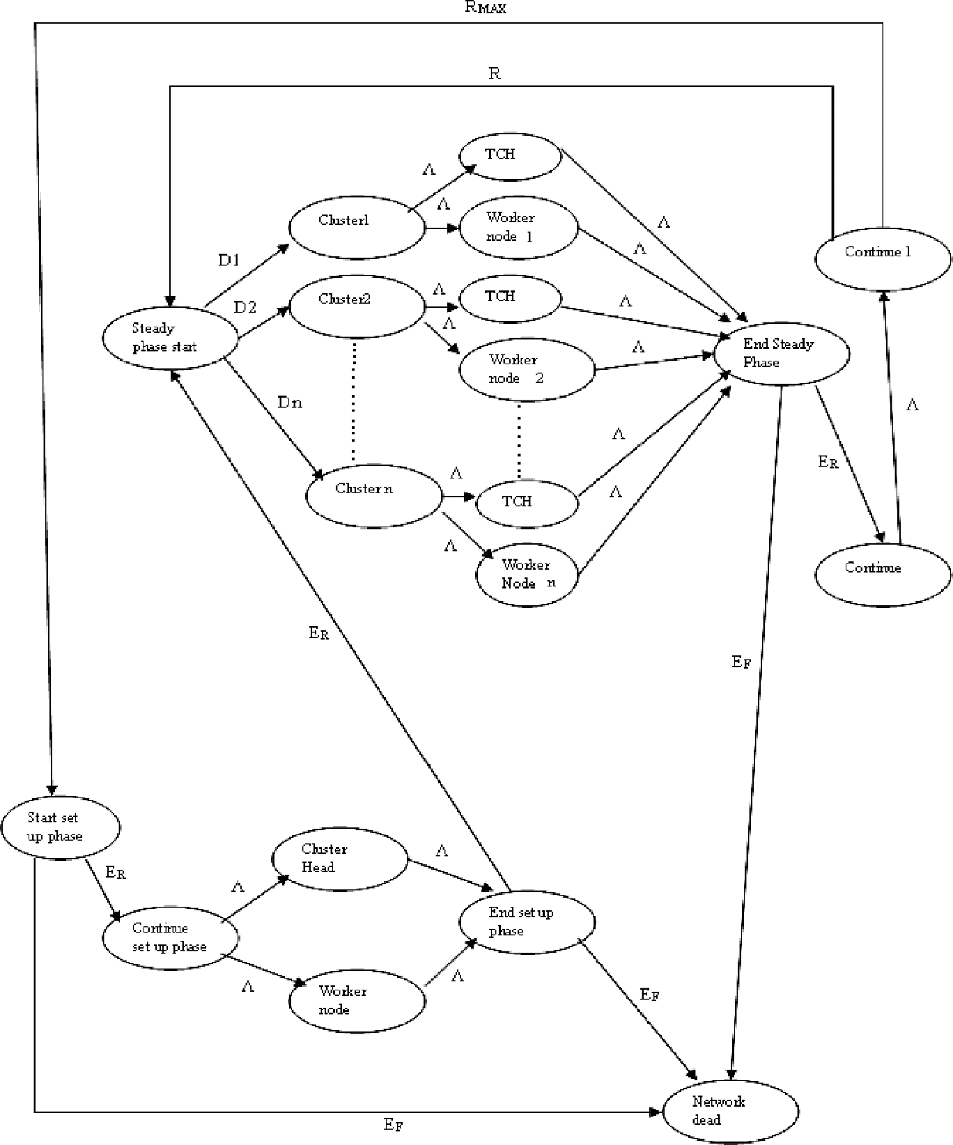
NFA of the proposed algorithm.

4.4. Simulation

In this section we evaluate the performance of the MEECHCP (Energy Efficient Cluster Head Communication Protocol) through simulation developed using Java programming language. We run a simulation of 100 nodes which are randomly dispersed in a field of 500 by 500 meter area. We place the base station just outside the field. The network is assumed to be homogenous with all the nodes having the same amount of energy that is 3 joule per node. The simulation of Leach and MEECHCP was performed on the same network deployment with same cluster head selection as well the message size is 1300 bytes. The radio model is the same as Leach [15] 50 nj to run the circuitry of both receiver and transmitter and 100 pj/bit to transmit. We reschedule the network after every 30 iterations. When the network is rescheduled new clusters are formed and new cluster heads are chosen.

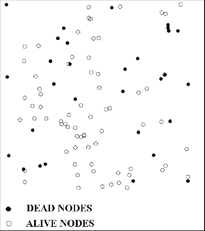
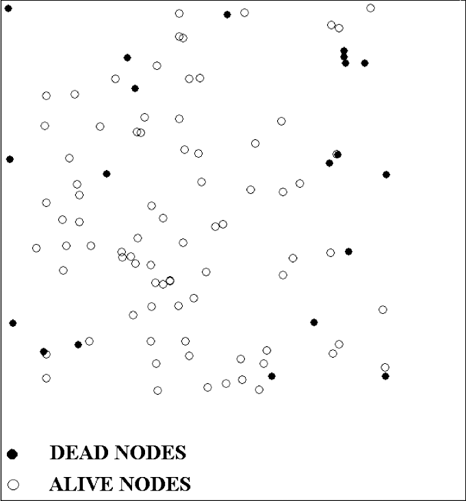
The network is randomly deployed as shown in Fig. 3. Figure 4 depicts the general operation of the protocol. First the nodes within the cluster transmit data to the cluster head via multihop then the cluster head transmits to sink via multihop. We run a simulation of the network 70 by 30 iterations. The graph from Fig. 5 shows the total amount of energy left in the entire network with respect to the number of iterations the simulation runs. Both the protocols were simulated using the same network cconfigurations, meaning the same node positions and the same cluster head selection. The graph clearly demonstrates that the proposed protocol has more energy left compared to Leach In Fig. 6 we show the number of nodes that were dead after running the network starting from 30 by 40 iterations to 30 by 70 iterations between Leach and MEECHCP. It is evident from the graph that the proposed algorithm ensures connectivity for a much longer period of time than Leach. Figure 7 shows the location of the nodes where they died in Leach after 30 by 70 itrations. From the figure we see that the top part has more dead nodes than the rest of the field compared with MEECHCP Fig. 8 where the dead nodes are more uniformly distributed across the field. The statistics collected from the simulation showed that after 70 by 30 iterations there were about 41 nodes dead in the network running Leach and the one running MEECHCP had 29 dead nodes.

Figure 3.

Random deployment of Sensor Network in the field.

Figure 4.

Protocol operation of MEECHCP.

Figure 5.

Total energy left in the network using Leach and MEECHCP.

Figure 6.

Comparisons of dead nodes between Leach and MEECHCP.

Figure 7.

Dead nodes in leach after 70 by 30 iterations.

Figure 8.

Dead nodes in MEECHCP after 70 by 30 iterations.

4.5. Multilayer Enhanced Energy Efficient Cluster Head Communication Protocol (MEEECHCP)

In this section we present a slight modification in the algorithm in order to make it more efficient and reliable. We know that computation is less expensive compared to transmission so we introduce in network compression as data travels within a cluster. We suppose that once a node has packet to be sent it can compress it by 23%. It means that the packet size to be transmitted is now 1000 bytes instead of 1300 bytes.

Figure 9 gives the energy left in the network with respect to the number of iterations the network runs. The graph clearly suggests that the introduction to compression within the clusters further enhances the algorithm from its previous version. Figure 10 gives a clear picture of the nodes that were dead when the network was running between 30 by 40 to 30 by 70 iterations using Leach, MEECHCP, and MEEECHCP protocol. To make things further clear we collected same statistics at different iterations of the simulation.

Figure 9.

Energy left in the network using MEECHCP and MEEECHCP.

Figure 10.

Dead nodes in Leach, MEECHCP, and MEEECHCP between 30 by 40 iterations to 70 by 30 iterations.

Table 3 gives the number of dead nodes during the simulation of Leach, EECHCP, and EEECHCP algorithms at certain iteration. The table shows that Leach has twice the number of dead nodes than the enhanced version of MEECHCP. The dead node distribution in MEEECHCP in field is shown in Fig. 10. After 2100 iterations the MEECHCP has 100% more nodes alive than Leach.

Figure 10.

Dead nodes in MEEECHCP after 70 by 30 iterations.

Table 3

Comparison of Dead Nodes between Leach, Meechcp, and Meeechcp

Protocol	No of iteration	No of Dead Nodes
Leach	900	17
Leach	2100	41
MEECHCP	900	10
MEECHCP	2100	29
MEEECHCP	900	9
MEEECHCP	2100	21

5. Conclusion and Future Work

It is obvious from the simulation results that the proposed algorithm compared to Leach is more energy efficient and also as the network progresses the network connectivity decreases in MEEECHCP and is less compared to Leach. This paper, like most of the previous approaches, is based on the assumption of error free radio transmission. The extension of this work will include simulation of WSNs with mobile nodes and to consider more realistic scenarios like simulating WSNs in a noisy environment. Also, we aim to analyse the different parameters affecting the performance of Sensor networks like MAC layer transmission technique along with the cluster size and trade off between the in network transmission and the in network computation.

Irfan Awan received his BSc from Gomal University, Pakistan (1986), MSc (Computer Science) from Qauid- e- Azam University, Pakistan (1990). He received his PhD from the Department of Computing, Bradford University, UK (1997). In 1999 he joined the Department of Computing, University of Bradford as a Lecturer and is a module coordinator for “Concurrent And Distributed Systems” and “Intelligent Network Agents”. His recent research lies in developing analytical tools for the performance of mobile and high speed networks Bradford. He has completed PGCHEP from the University of Bradford in 2002 and has gained an ILT membership.

Nauman Israr received his BCS (bachelor of computer science) from Pakistan Air Force College (Fazaia Degree College Risalpur) Risalpur in 2005. He is now pursuing his PhD in the Department of Computing, University of Bradford. His research interest includes wireless sensor networks, especially the clustering techniques in Wireless sensor networks.

References

Min

R. B.

Cho

Shih

S. -H.

Sinha

Wang

Chandrakasan

, “Low-power wireless sensor networks,” in Proceedings of 14th International Conference on VLSI Design (VLSI DESIGN 2001), pp. 205–210, 2001.

Rabaey

E. A. J.M.

, “Pico Radio support ad hoc ultra low power wireless networking,” IEEE Computer, vol. 33, pp. 42–48, July 2000.

Kahn

J. M. K.

Pister

R.H.

Pister

K.S.J.

, “Mobile networking for “Smart Dust,” 5th Annual ACM/ IEEE International Conference on Mobile Computing and Networking (MobiCom'99)”, pp. 271–278, 1999.

Werff

D. T. J. V. d.

, “Global future report,” in Technology Review, 2003. Available at: http://www.globalfuture.com/mit-trends2003.htm.

Haenggi

, “Opportunities and Challenges in Wireless Sensor Network,” in Handbook of Sensor Networks Compact Wireless and Wired Sensing Systems: CRC press, 2005, pp. 21–34.

Akyildiz

W. S. I.F.

Sankarasubramaniam

, and Cayirci

, “Wireless sensor network: a survey” Computer Networks, pp. 393–422, 2002.

Al-Karaki

J. N.

and Kamal

A. E.

, “Routing techniques in wireless sensor networks: A survey,” IEEE Wireless Communications, vol. 11, p. 6, 2004.

Mainwaring

R. S. A.

Anderson

Polastre

, “Wireless Sensor Networks for Habitat Monitoring,” Proceedings of the 1st ACM International Workshop on Wireless Sensor Networks and Applications, pp. 88–97, 2002.

Bonnet

G. P.

Seshadri

, “Querying the physical world,” IEEE Personal Communication, 2000.

10.

Younis

K. A. a. M.

, “A survey on routing protocols for wireless Sensor network,” Journal of Adhoc Networks, vol. 3, pp. 325–349, 2005.

11.

Ibriq

I. M. Jamil

, “Cluster based Routing in Wireless Sensor Network: Issues and Challenges,” The Society for Modelling and Simulation International SSC Digital Library.

12.

Heinzelman

A. C. A. H. B. W.

, “Energy-Efficient Communication Protocol for Wireless Micro sensor Networks,” Proc. 33rd Hawaii Int'l. Conf. Sys. Sci., 2000.

13.

Intanagonwiwat

R. G. A. D. E. C.

, “Directed diffusion: A scalable and robust communication paradigm for sensor networks,” presented at 6th Annual ACM/IEEInternational Conference on Mobile Computing and Networking (MobiCom'00), Boston, MA, 2000.

14.

Heinzelman

, “Application Specific Protocol Architecture for Wireless Sensor Network,” PhD: Massachussetts Institute of Technology, 2000.

15.

Agrawal

A. M. A. D. P.

, “TEEN: A Protocol for Enhanced Efficiency in Wireless Sensor Networks,” in Proceedings of 1st International Workshop on Parallel and Distributed Computing Issues in Wireless Networks and Mobile Computing, 2001.

16.

Agrawal

A. M. A. D. P.

, “ATEEN: A Hybrid protocol for efficient routing and comprehensive information retrieval in wireless sensor networks,” in Proceedings of 2nd International Workshop on Parallel and Distributed Computing Issues in Wireless Networks and Mobile Computing, 2002.

17.

Gupta

, “Load-balanced clustering of wireless sensor networks,” Anchorage, AK, United States, 2003.

18.

Muraganathan

D. C. F. M. S. D.

Bhasin

R. I.

and Fapojuwo

A. O.

, “A centralized energy-efficient routing protocol for wireless sensor networks,” Communication Magazine, IEEE, pp. 8–13, 2005.

19.

Hansen

J. N. Ewa

Nolin

Mikael

Björkman

Mats

, “Efficient Cluster Formation for Sensor Networks,” MRTC Report ISSN 1404–3041 ISRN MDH-MRTC-199/2006–1-SE, Mälardalen Real-Time Research Centre, Mälardale University, 2006.

20.

Israr

Nauman

and Awan

Irfan

“Energy efficient intra cluster head communication protocol”

6^th Annual Post Graduate Symposium on the Convergence of Telecommunications, Networking, and Broadcasting Liverpool John Moores University, UK, June 2006, pp. 285–290.

Multilayer Cluster Based Energy Efficient Routing Protocol for Wireless Sensor Networks