
Abstract
In delay tolerant networks, the success rate and the transmission speed are restricted by limited social interaction and complex node mobility pattern analysis. To increase the success rate and reduce the transmission delay in delay tolerant networks, we propose Daily Routine Analysis for Node Searching in delay tolerant networks. In Daily Routine Analysis for Node Searching, each node is required to generate a Staying Probability Table and a Transiting Probability Table by analyzing its own daily routine, then to distribute its Staying Probability Table and Transiting Probability Table to the whole network with the help of other nodes having different mobility patterns. On the basis of the Staying Probability Table and Transiting Probability Table, Daily Routine Analysis for Node Searching further provides a node tracking strategy and an opportunistic routing strategy for delivering data from the source node to the destination node. Trace-driven experiments are performed to compare Daily Routine Analysis for Node Searching with previous node searching methods. The experimental results demonstrate that Daily Routine Analysis for Node Searching is able to promote the success rate and reduce the transmission delay effectively.
Introduction
With the popularization of mobile devices in all kinds of application scenarios, delay tolerant networks (DTNs) as a novel type of communication paradigm have attracted lots of interests from the academic to the industry. 1 In DTNs, nodes are connected intermittently and there is no constant end-to-end path, which makes the design of routing methods become a challenge problem. Existing DTN routing algorithms2–13 utilize different feature information, such as past encounter records (probabilistic routings), social network properties (social network based routings), and past moving paths (location based routings), to estimate nodes’ probabilities to meet the destination node.
Recently, to break through the limitations in existing routing methods and make combination of their advantages, some node searching algorithms for DTNs have been proposed.14–16 DTN-FLOW 14 utilizes nodes’ transiting probabilities among different geographical subareas and chooses nodes that are most likely moving closer to the destination node as relay nodes, and this method can not only reduce the transmission delay but also promote the success rate. DSearch 15 tracks the destination node with the help of both the geographical transiting information and nodes’ long-term staying probabilities, and it shows greater transmission reliability than the routing methods by only depending on geographical information or meeting probabilities. In TSearch, 16 nodes can play different roles, have preferred subareas, and share encounter information and meeting probabilities, so all the three factors, such as meeting probability, social relationship, and geographical information, are taken into consideration in routing decision.
Even these node searching methods do bring some effective and positive influence on success rate promotion and transmission delay reduction; however, there are still some problems need to be solved: (1) in DTN-FLOW, 14 the transiting probability is obtained by predicting and the node flows between subareas are not time related, which may not be reliable for real-time node searching; (2) in DSearch, 15 it is not practical and convenient to require each node to leave a hint about where it will go before it leaves its current subarea, because a node may change its route at any time or not surely know where it will go; and (3) in TSearch, 16 it may happen that all friends and encounters of a source node know nothing about its destination node, which means the help from friends and encounters is limited and cannot make sure every node is always traceable for other nodes.
So, in order to overcome the above drawbacks, we propose Daily Routine Analysis for Node Searching (DRANS) in DTNs. In DRANS, each node is required to generate a Staying Probability Table (SPT) and a Transiting Probability Table (TPT) by analyzing its own daily routine. The SPT and TPT are time-related and helpful for real-time node searching. To make every node traceable, each node is also required to store its original SPT and TPT in subareas where it visits frequently and stays in habitually, and distribute its simplified SPT and TPT to subareas where it has never been with the help of other nodes.
On the basis of the SPT and TPT, DRANS further provides two kinds of node searching strategies: node tracking strategy and opportunistic routing strategy. In DRANS, the subarea where a source node is currently staying is defined as its current subarea, the subarea where a destination node is most likely staying currently is chosen as a target subarea, and the subareas where a node visits frequently and stays in habitually are defined as its preferred subareas. While a source node delivers data to a destination node, if the source node’s current subarea is a preferred subarea for the destination node and has the destination node’s original SPT and TPT, the node tracking strategy can help the source node to track the destination node; otherwise, the opportunistic routing strategy needs to be performed. In the node tracking strategy, the destination node can be tracked along its transiting routes recorded in its original TPT. In the opportunistic routing strategy, for delivering data from the source node’s current subarea to the target subarea, opportunistic forwarding paths and forwarding nodes are determined according to nodes’ SPT and TPT.
The main contributions of this work are summarized as follows:
To break through the constraint of limited social interaction and make sure each node is traceable for other nodes, each node is required to generate a SPT and a TPT via daily routine analysis and distribute them to subareas where it has never been.
Aware of that the long-term staying probability and transiting probability in previous studies are not time related, we define a time-related short-term staying probability additionally that can provide a more precise description of node mobility pattern and help us to obtain time-related transiting probability.
To speed up the distribution of SPT and TPT, we define two kinds of mobility dissimilarities. According to the mobility dissimilarities, a node can easily find out other nodes having different mobility patterns and let them distribute its SPT and TPT to its unknown subareas.
Based on the SPT and TPT, a node tracking strategy and an opportunistic routing strategy are designed. In the node tracking strategy, for determining whether a destination node is still in a subarea, each node is required to report its visiting records when it enters and leaves a subarea. In the opportunistic routing strategy, for determining forwarding paths, a subarea delivering ability metric related to node flows and distances between subareas is defined; meanwhile, for selecting forwarding nodes, a node delivering ability metric related to nodes’ short-term staying probabilities is also defined.
The rest of the article is organized as follows. In section “Related work,” an overview of related work is presented. In section “Network model and daily routine analysis,” we explain how to perform the daily routine analysis and distribute its result. In section “Details of node searching in DRANS,” the two kinds of node searching strategies in DRANS are discussed in detail. And the performances of DRANS are evaluated and analyzed in section “Performance evaluation.” In section “Conclusion,” we conclude the work and give a future research direction.
Related work
Routings in DTNs
The existing routing methods for DTNs are mainly classified into three categories: the probabilistic routings,2–5 the social network–based routings,6–11 and the location-based routings.11–13
The probabilistic routing methods use nodes’ past encounter records to predict their future encounter probabilities and choose the nodes with higher probabilities to meet destination nodes as relay nodes. In PROPHET, 2 both the direct encountering probabilities and indirect relay chances are considered, the encountering probabilities are updated upon encounter frequency and aged over time. MaxProp, 3 RAPID 4 and MaxContribution 5 extend PROPHET by further specifying forwarding and storage priorities of different packets based on their probabilities of successful delivery. RAPID 4 and MaxContribution 5 calculate the priorities of packets with different goals such as minimal delay and maximal bit rate, respectively.
The social network–based routing methods consider the social relationships between nodes, as well as social properties such as centrality and similarity while delivering data. In BUBBLE, 6 each node has two ranks: global and local; the global rank brings data to its destination community and the local rank helps the data to find its destination node within the destination community. Peoplerank 7 provides a ranking method using tunable weighted social information in which nodes get higher weight if they are socially connected to other important nodes in the network. SimBet 8 defines the social network analysis metrics: betweenness centrality and similarity based on nodes’ past interactions for efficient data delivery in DTNs. OFPC 9 defines the relative importance of a node to a group of nodes as partial centrality and designs an opportunistic forwarding scheme with the partial centrality. Mei et al. 10 and Leguay et al. 11 provide methods to calculate nodes’ similarity in different aspects.
The location-based routing methods record nodes’ historical geographical information and research nodes’ mobility patterns. GeoDTN 12 uses historical movement information to predict the possibility of two nodes becoming neighbors and forwards data to nodes more likely to be a neighbor of the destination node. PGR 13 analyzes nodes’ mobility patterns to predict their future movements while choosing forwarding nodes. In MobyPoints, 11 the similarity of meeting probabilities in different locations is defined and packets are forwarded with considering this similarity between relay nodes and the destination node.
Opportunistic routings for wireless mesh networks
Unreliable and unpredictable wireless medium makes traditional routing methods no longer applicable. To overcome this problem, the concept of opportunistic routing has been proposed. 17 Different from the traditional best path routing, opportunistic routings allow multiple neighbors that can overhear the transmission to participate in forwarding packets, and effectively combine the multiple neighbor links into a strong link.
ExOR 18 is a seminal opportunistic routing protocol, in which each packet contains a forwarding list including nodes that can potentially forward it and the nodes in the forwarding list relay data packets according to ETX metric 19 instead of physical distance. SOAR 20 proposes a simple opportunistic adaptive routing protocol, which explicitly supports multiple simultaneous flows by strategically selecting forwarding nodes and employing adaptive rate control. ROMER 21 is another opportunistic routing protocol to forward packets simultaneously along multiple paths and it provides a credit-based scheme to limit the number of transmissions. CORMAN 22 extends ExOR to disclose a cooperative opportunistic routing scheme allowing that route information is updated by intermediate forwarders. In CORMAN, when a flow of data packets is forwarded to their destination, its forwarding list may be adjusted corresponding to updates of the route information during transmission, and the updated information is propagated upstream rapidly, so that all upstream nodes learn about the new route at a rate much faster than via periodic route exchanges.
This article learns the advantages of both probabilistic routings and social network–based routings. It takes use of nodes’ social properties to do daily routine analysis and calculates nodes’ time-related staying probabilities and transiting probabilities to provide a more precise description of node mobility pattern. Furthermore, on the basis of the daily routine analysis result and enlightened by the existing opportunistic routing protocols, this article designs a node tracking strategy and an opportunistic routing strategy for delivering data from the source node to the destination node.
Network model and daily routine analysis
In order to describe the two kinds of node searching strategies clearly in the following sections, we define the network model and discuss the details of daily routine analysis in this section. The notations used in this article are listed in Table 1 as follows.
Notations.

Network model
We implement DRANS in a DTN with mobile nodes having limited communication range and storage space. The DTN is assumed to have a small or medium network scale–like DART 23 and DNET. 24 In the DTN, the spots where the mobile nodes visit frequently are called popular places, and the popular places are assumed to be distributed relatively evenly. The whole DTN is split into subareas according to the popular places. Specifically, each subarea contains one popular place. The mobile nodes are denoted by Ni and the subareas are denoted by Ai.
Landmarks. We configure each subarea with a landmark which is a central station having large storage space and powerful processing capability. Each landmark has a redundant landmark. If a landmark fails, its redundant landmark will replace it to keep the whole system working normally. The landmarks cannot communicate with each other directly, but they can communicate with each other indirectly through the mobile nodes and have responsibility to store and process the information sent by the mobile nodes.
Communication between the mobile nodes and the landmarks. In a subarea, if the distance between a node and a landmark is less than the node’s transmission range, the node can communicate with the landmark directly; otherwise, the node communicates with the landmark indirectly through other nodes moving close to the landmark.
Daily routine analysis
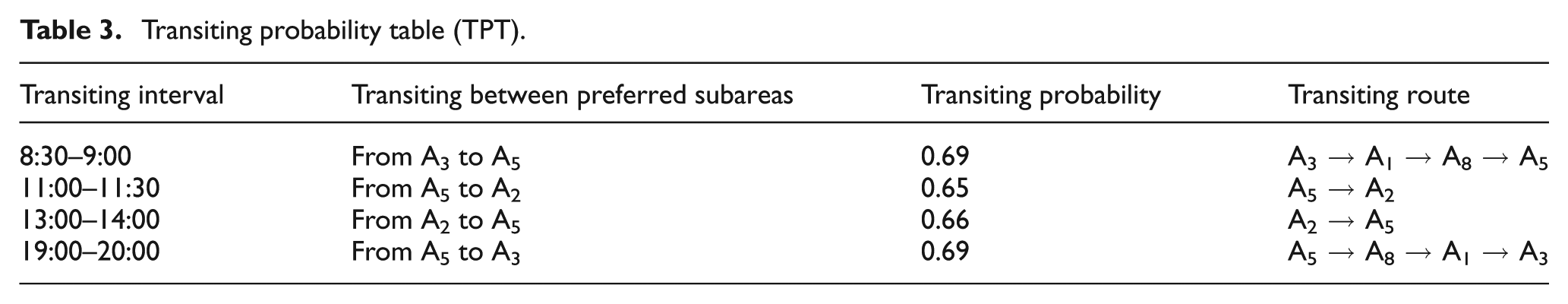
To obtain nodes’ mobility patterns in the DTN, we require each node to record its daily routine. A node’s daily routine includes the subareas where it has been and the corresponding time when it enters and leaves them. Via analysis of the daily routine, each node generates a SPT and a TPT. For providing a simple and clear illustration, the typical forms of the SPT and the TPT are shown in Tables 2 and 3, respectively.
Staying probability table (SPT).

Transiting probability table (TPT).
SPT
In view of that the long-term staying probability in DSearch 15 is not time related and cannot reflect the change of node mobility pattern with time, we define a time-related short-term staying probability additionally which shows the probability of a node staying in a subarea in a specific interval of time.
In Table 2, a node’s SPT shows its preferred subareas, and the staying intervals, the short-term staying probabilities, and the long-term staying probabilities in its preferred subareas. In some applications, a node’s staying intervals may overlap each other and a node may have more than one preferred subarea in a staying interval.
Preferred subarea. Different nodes have different society properties and daily routines. By analysis of a node’s daily routine, it can be found that the node may visit or stay in some subareas every day. The subareas where a node visits frequently and stays in habitually are called its preferred subareas.
Staying interval. Each node divides a day (24 h) into staying intervals and transiting intervals according to its own daily routine. The time gap between two adjacent staying intervals is a transiting interval and can be recorded in the TPT. The start time and the end time of each interval are the average values of the statistical results. Ni’s time intervals are denoted by
Short-term staying probability. In a staying interval, for a node, there may be more than one possible subarea to go, so a node may have more than one short-term staying probability in a specific interval of time. A node’s short-term staying probability in a subarea in an interval depends on the average time it stays in this subarea in the interval. For instance, if the average time of Ni staying in Am in interval

In each staying interval, the sum of a node’s short-term staying probabilities in all possible preferred subareas is 1.
4. Long-term staying probability. The SPT also includes a node’s long-term staying probability in a subarea in an interval. A node’s long-term staying probability in a subarea in an interval also depends on the average time it stays in this subarea in the interval. For instance, if the average time of Ni staying in Am in interval
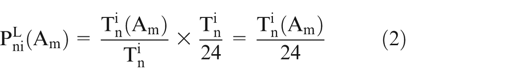
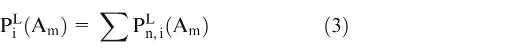
We also calculate a node’s long-term staying probability in a subarea for a whole day, for analyzing nodes’ mobility dissimilarities that will be discussed in subsection “Distributing and updating of simplified SPT and TPT” of section “Daily routine analysis.” And as shown in formula (3), the long-term staying probability of Ni staying in Am for a whole day is
Both the short-term staying probability and the long-term staying probability contribute to data delivery and node searching in different ways. Subsequently, the short-term staying probability is used to calculate nodes’ transiting probabilities, and the long-term staying probability helps to distribute the SPT and TPT.
TPT
As shown in Table 3, a node’s TPT includes the node’s transiting intervals, transiting probabilities, and transiting routes among its preferred subareas.
Transiting interval. A node not only spends time on staying in its preferred subareas but also on transiting among them. The start time and the end time of each transiting interval are also the average values of the statistical results.
Transiting probability. To find out whether Ni transits from Am to Ah in a specific interval of time, we should figure out whether Ni has stayed in Am before the interval and will go to Ah after the interval. Therefore, the transiting probability of Ni transiting from Am to Ah in interval

3. Transiting route. It can be observed that, for a node, there may be more than one transiting route from one preferred subarea to another; in other words, the node may choose different transiting routes while transiting. So, here, the TPT records all possible transiting routes of a node in each transiting interval.
The transiting probability is calculated according to the short-term probability and thus, it is time related. The transiting routes and the transiting probabilities in the TPT can be used by landmarks separately to conduct node tracking and compute node flows between different subareas in section “Details of node searching in DRANS.”
Simplified SPT and TPT
To reduce the storage burden of landmarks and overhead on distributing the SPT and TPT, a short-term staying probability threshold and a long-term staying probability threshold are configured. Each node is required to compress its original SPT into a simplified SPT, by filtering out the short- and long-term staying probabilities that are less than the corresponding threshold from its original SPT. Each node also curtails its original TPT into a simplified TPT according to the two thresholds. The two thresholds can be adjusted according to their effects on network performances, which will be discussed in detail in section “Experimental setup.”
Each node should keep its original TPT and SPT in the preferred subareas included in its simplified SPT, and only needs to distribute its simplified SPT and TPT to the subareas that are not included in its simplified SPT.
Distributing and updating of simplified SPT and TPT
For distributing the simplified SPT and TPT, each node is required to maintain two subarea sets: a distributed subarea set and an undistributed subarea set. For a node, the subareas already having its SPT and TPT (original or simplified) are put into its distributed subarea set, and the subareas without its SPT and TPT are put into its undistributed subarea set. The distributed subarea set and the undistributed subarea set of Ni are denoted by
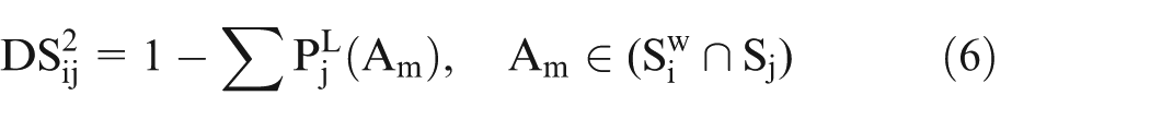
We define the subareas where a node has never been as its unknown subareas. While a node distributes its simplified SPT and TPT to its unknown subareas, it needs the help from other nodes. We notice that, for a node, the other node having more different mobility pattern gets higher probability going to its unknown subareas; in other words, the other node having greater mobility dissimilarity is more capable of helping this node to distribute its SPT and TPT. Thus, we define two kinds of mobility dissimilarities which are called the first dissimilarity and the second dissimilarity. These two kinds of dissimilarities represent the mobility pattern difference between nodes from different aspects, but both of them are related to the long-term staying probability.
For instance, there are two nodes Ni and Nj, Sj is the subarea set including Nj’s preferred subareas in its simplified SPT,

Furthermore, a method to distribute the simplified SPT and TPT is designed according to the two kinds of mobility dissimilarities. Here, to make a clear illustration, we take Ni using this method as an example. The process of Ni implementing this method includes the following three steps:
Step 1. Ni distributes its simplified TPT and SPT to the subareas not included in its simplified SPT but on its transiting routes, and then, it transfers these subareas from its undistributed subarea set to its distributed subarea set.
Step 2. After step 1, if there are still subareas left in Ni’s undistributed subarea set
Step 3. After step 2, if there are still some subareas left in
The algorithm to select the first distribution ambassadors

When a distribution ambassador of Ni (the first or the second distribution ambassador) reaches a subarea without Ni’s simplified SPT and TPT, it immediately transmits Ni’s simplified SPT and TPT to the subarea’s landmark directly or through other nodes indirectly.
For a node, after each time updating its original SPT and TPT, it is required to immediately distribute its new simplified SPT and TPT to all subareas. Obviously, excessively frequent updating of the SPT and TPT may cause an unbearable transmission overhead burden, thus DRANS desires each node has a stable mobility pattern.
It should be emphasized that, the staying probability in the SPT and the transiting probability in the TPT are different from those defined in the existing studies.14,15 In DTN-FLOW, 14 each node obtains its own transiting probability by predicting and maintains it by itself, which aims to help landmarks to forward packets to neighbor subareas. In DRANS, the transiting probability is calculated according to the short-term staying probability that is time related, which is maintained by landmarks and distributed to the whole network for node searching. Although DSearch 15 has already defined the long-term staying probability, in the SPT, we define the short-term staying probability additionally which is time-related and more helpful for real-time node searching. In addition, our method to distribute the SPT and TPT can make sure every node is traceable for other nodes in the network, which makes DRANS outperform the node tracking method based on limited help of friends and encounters in TSearch. 16
Details of node searching in DRANS
In this section, we discuss how a source node searches a destination node according to the destination node’s daily routine analysis result. There are two different situations for the node searching.
The first situation is that the source node’s current subarea is a preferred subarea in the destination node’s simplified SPT, that is, the source node’s current subarea has the destination node’s original SPT and TPT. In this situation, DRANS uses a node tracking strategy to track the destination node along its transiting routes with the help of its original SPT and TPT.
The second situation is that the source node’s current subarea is not a preferred subarea in the destination node’s simplified SPT; in other words, the source node’s current subarea only has the destination node’s simplified SPT and TPT. In this situation, DRANS chooses the subarea where the destination node is most likely staying at the current interval of time as a target subarea, and then performs an opportunistic routing strategy to determine forwarding paths and forwarding nodes for delivering data from the current subarea to the target subarea.
An exemplary scenario of the two different situations is shown in Figure 1. In Figure 1, N1 and N2 are two different source nodes, N3 is a destination node, and the blue subareas A8 and A11 are preferred subareas in N3’s simplified SPT. If N2 wants to deliver data to N3, since N2’s current subarea A8 is a preferred subarea in N3’s simplified SPT, which has N3’s original SPT and TPT, the landmark of A8 can use the node tracking strategy to track N3 along N3’s transiting routes with the help of N3’s original SPT and TPT. But while N1 sends data to N3, due to N1’s current subarea A1 only having N3’s simplified SPT and TPT, the landmark of A1 has to choose A11 where N3 is most likely staying at the current interval of time as a target subarea and performs the opportunistic routing strategy between the current subarea A1 and the target subarea A11. The details of the node tracking strategy and the opportunistic routing strategy are discussed in section “Node tracking strategy” and section “Opportunistic routing strategy,” respectively.

A scenario of two different situations in node searching.
Node tracking strategy
To implement the node tracking strategy, landmarks are configured to record and update the visiting records of each node. Specifically, when a node enters and leaves a subarea, it needs to report the entering time and the leaving time for the subarea to the subarea’s landmark, and the landmark only records the node’s last entering time and leaving time as its visiting records. The last time of Ni entering and leaving subarea Ai are denoted as TE(Ni)(Ai) and TL(Ni)(Ai), respectively.
It needs to be explained that our visiting records are different from those defined in DSearch. 15 In this article, a node’s visiting records in a subarea show the latest time when it enters and leaves the subarea, which are maintained by the subarea’s landmark and can be used to determine whether the node is still staying in the subarea or not. However, in DSearch, 15 a node generates a visiting record before it enters a new subarea, and the visiting record is a hint telling the node’s new subarea. The visiting record in DSearch 15 may not be always available for a node, because a node may hardly determine when to leave and where to go in some practical applications.
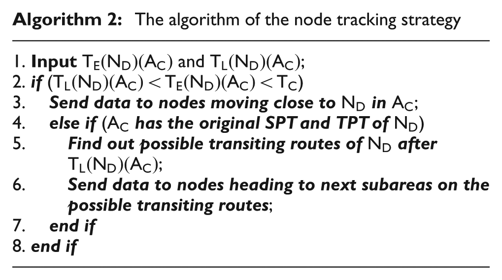
How to use the visiting records in the node tracking strategy is shown in Algorithm 2. TC denotes the time when Algorithm 2 is operated, NS and ND represent a source node and a destination node, respectively, AC denotes the subarea where the source node NS is currently staying. In Algorithm 2, if TL(ND)(AC) < TE(ND)(AC) < TC, it means that ND is still in AC and NS can send data to ND through nodes moving close to ND. If TE(ND)(AC) < TL(ND)(AC) < TC, it means that ND has already left AC, and furthermore, if AC has ND’s original SPT and TPT, the landmark of AC can find out ND’s possible transiting routes according to its original TPT and track ND along the subareas on its possible transiting routes.
The algorithm of the node tracking strategy
We take the scenario shown in Figure 2 as an example to illustrate the details of the node tracking strategy in Algorithm 2. In Figure 2, N4 in A5 wants to deliver data to N5 and sends a data delivery request to the landmark of A5. After receiving the request, the landmark of A5 finds that N5 is not in A5 based on N5’s visiting record, but it has the original SPT and TPT of N5, then it checks all the possible transiting routes of N5, and gets that N5 has three possible transiting routes after leaving A5: A5→A6→A7→A8, A5→A10→A11, and A5→A9→A13, so the landmark of A5 sends data to nodes heading to A6, A9, and A10.

Illustration of the node tracking strategy.
If the landmark of A10 has a visiting record of N5 that is newer than N5’s visiting records in A5, it continues to track N5 along A10→A11, and the landmarks in A6 and A9 then stop tracking N5 for they having no newer visiting record of N5. But it may happen that all the landmarks of A6, A9, and A10 cannot find a newer visiting record of N5. If this happens, the landmark of A5 will receive failure feedbacks from all the landmarks of A6, A9, and A10 and needs to broadcast tracking packets to all of its neighbor landmarks.
Opportunistic routing strategy
If a source node wants to deliver data from its current subarea to a destination node, but its current subarea only has the simplified SPT of the destination node, the landmark of its current subarea needs to perform the opportunistic routing strategy between the current subarea and the target subarea where the destination node is most likely staying at the current interval.
In the opportunistic routing strategy, the landmark of the current subarea calculates node flows between different subareas according to all SPT and TPT it has and determines a certain number of forwarding paths from the current subarea to the target subarea. The subareas on the determined forwarding paths are called forwarding subareas and put into a forwarding subarea list. Nodes that are most likely heading to the forwarding subareas are put into a candidate forwarding node list. The number of forwarding paths can be configured and adjusted by users according to their demands. For instance, in Figure 3, N6 in A1 wants to deliver data to N7, it sends a data delivery request to the landmark of A1. Here, the landmark of A1 only has N7’s simplified SPT, so it analyzes N7’s simplified SPT to find that N7 has a great short-term staying probability in A16 at the current interval of time, and then chooses A16 as a target subarea. The landmark of A1 performs the opportunistic routing strategy between A1 and A16, and finds out three forwarding paths for data delivering from A1 to A16: A1→A6→A11→A16, A1→A6→A7→A11→A16, and A1→A5→A10→A15→A16, then puts the subareas on these three forwarding paths into its forwarding subarea list. The detailed forwarding path determining method is described in section “Forwarding path determining.”

Illustration of the opportunistic routing strategy.
Forwarding path determining
In order to determine the forwarding paths from the current subarea to the target subarea, the landmark of the current subarea first analyzes all SPT and TPT (original and simplified) it has and calculates the node flow between every two adjacent subareas according to formula (7)

In formula (7), Fn(Am→Ah) denotes the node flow between two adjacent subareas Am and Ah in an interval of time, which is the sum of the transiting probabilities of nodes transiting from Am to Ah in the interval. The node flow is dependent on the transiting probabilities of nodes and especially time related, which is more helpful for real-time node searching.
For obtaining reliable forwarding paths, we define a subarea delivering ability metric related to the node flow and the communication distance between every two adjacent subareas. The subarea delivering ability metric can be calculated according to formula (8)

In formula (8), SDn(Am→Ah) represents the subarea delivering ability metric between two adjacent subareas Am and Ah, which is proportional to the node flow between Am and Ah while inversely proportional to the distance between Am and Ah. The subarea delivering ability metric between two adjacent subareas is greater, and the data delivery hop between the two adjacent subareas is more reliable accordingly.
We also define a path delivering ability metric to represent a path’s reliability, which is equal to the product of subarea delivering ability metrics of all its hops. The path (from the current subarea to the target subarea) having a greater path delivering ability metric gets a greater probability to be a forwarding path.
Forwarding node selection
Subareas on the determined forwarding paths are put into a forwarding subarea list. For delivering data through the determined forwarding paths, we should select the nodes most likely heading to the subareas in the forwarding subarea list as candidate forwarding nodes. In order to promote the success rate and select reliable candidate forwarding nodes, we define a node delivering ability metric related to nodes’ short-term staying probabilities.
We use

If a node has a higher node delivering metric for a source node, it gets a greater probability to be selected as the source node’s candidate forwarding node. And all candidate forwarding nodes of a source node are put into its candidate forwarding node list.
To reduce transmission delay and further select reliable forwarding nodes from the candidate forwarding node list, we define a transmission delay metric. The candidate forwarding node having a smaller transmission delay metric gets a greater probability to be finally selected as a forwarding node. The number of forwarding nodes also can be configured and adjusted by users according to their demands.
If

In the forwarding node selection, it is allowed that two source nodes select the same node as their forwarding node.
Data transmission and strategy adjustment
When a forwarding node arrives at the first preferred subarea after leaving its previous preferred subarea where it has taken a forwarding mission, and if it finds the current preferred subarea is not in the mission’s forwarding subarea list, it must report this failure to the landmark of the previous preferred subarea through nodes heading back. In the extreme case, for a forwarding mission, if all its forwarding nodes fail, the opportunistic routing strategy needs to be performed again.
If a forwarding node enters into a subarea in its mission’s forwarding subarea list, it will transfer its forwarding mission to the subarea’s landmark. And if the subarea is in the destination node’s simplified SPT, its landmark will perform the node tracking strategy for further data delivering; otherwise, its landmark will continue to perform the opportunistic routing strategy from the subarea to the target subarea by further determining forwarding paths and selecting forwarding nodes. While a forwarding node arrives at the target subarea, and if the destination node is not in this target subarea, the target subarea’s landmark will continue to perform the node tracking strategy for further searching.
It is obvious that our routing strategy based on the node flow is also different from that in DTN-FLOW. 14 It introduces the conception of opportunistic routing, defines the delivering ability metrics about forwarding paths and forwarding nodes, and provides the method to select the forwarding nodes. Importantly, it allows the strategy adjustment between the node tracking strategy and the opportunistic routing strategy.
Performance evaluation
Experimental setup
Our experiments are conducted using DART trace 23 and DNET trace. 24 DART trace records communication of wireless devices carried by the students on Dartmouth College campus. DNET trace records association of WiFi nodes attached to the buses in the downtown area of UMass college town. We filter out nodes with few records and short connections to retain 320 nodes and 159 subareas in DART and 34 nodes and 18 subareas in DNET. In both DART trace and DNET trace, we set an initial period during which nodes can collect daily routine information to generate the SPT and TPT. After the initial period, source nodes are generated according to search rate and then they randomly choose destination nodes to deliver data.
As mentioned in section “Daily routine analysis,” we compress the original SPT and TPT into the simplified SPT and TPT according to the short- and long-term staying probability thresholds, respectively. For determining appropriate values of the two thresholds, we conduct simulations to observe how these two thresholds affect the success rate and the transmission overhead of DRANS when other parameters are fixed. The simulation results are shown in Figures 4–7.
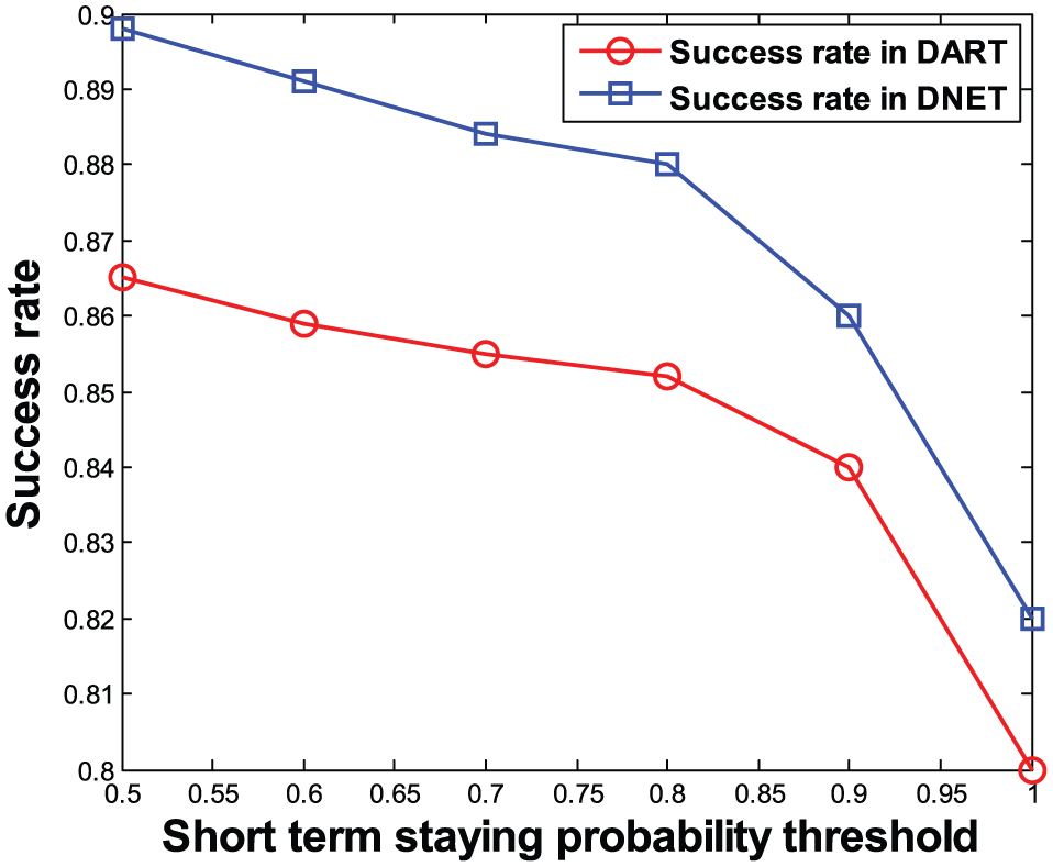
Effect of short-term staying probability threshold on success rate.
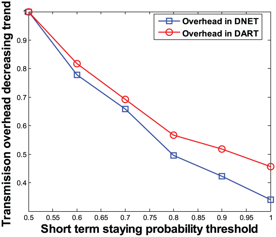
Effect of short-term staying probability threshold on transmission overhead.

Effect of long-term staying probability threshold on success rate.
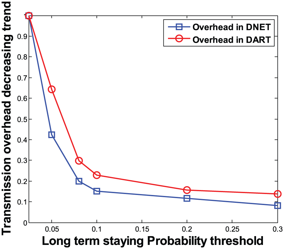
Effect of long-term staying probability threshold on transmission overhead.
Figures 4 and 5 show the trends of success rate and transmission overhead under different short-term staying probability thresholds in DART and DNET, respectively. From Figure 4, it can be seen that the success rate goes down with the increase in the short-term staying probability threshold. Especially, when the short-term staying probability threshold is higher than 0.8, the success rate drops faster as the short-term staying probability threshold increases. But Figure 5 tells us that increase in the short-term staying probability threshold is beneficial for reducing the transmission overhead.
Figures 6 and 7 show the trends of success rate and transmission overhead under different long-term staying probability thresholds in DART and DNET, respectively. From Figures 6 and 7, it can be seen that with the increase in the long-term staying probability threshold, both the success rate and the transmission overhead go down. Especially, with the long-term staying probability threshold being higher than 0.08, the transmission overhead decreases dramatically.
Based on the above simulation results, to achieve balance between the success rate and the transmission overhead, the short- and long-term staying probability thresholds are configured to 0.8 and 0.08 in subsequent simulations, respectively.
Experimental results
We evaluate DRANS with different number of forwarding paths and forwarding nodes. DRANS with three forwarding paths and three forwarding nodes is denoted by DRANS1, while DRANS with five forwarding paths and five forwarding nodes is denoted by DRANS2.
We compare DRANS with DSearch 15 (denoted by DS) and TSearch 16 (TSearch without and with encounter recording exchanges are denoted by TS1 and TS2, respectively) in the following four aspects: (1) success rate: the percentages that the source nodes successfully deliver data to their destination nodes, (2) average delay: the average time cost by the source nodes to deliver data to the destination nodes, (3) average transmission overhead: the average number of packets transmitted among nodes, and (4) average memory usage: the average amount of memory unit used by each node.
Success rate
Figures 8 and 9 show the success rates of different methods under different search rates in DART and DNET, respectively. In both DART and DNET, the success rate of DRANS is higher than that in all other methods. DRANS outmatches TS1 and TS2 in the success rate promotion, because it breaks through the success rate restriction caused by the limited social interaction. The success rate of DRANS is higher than that in DS, which demonstrates that the SPT and TPT in DRANS are more efficient for node searching than the mobility pattern table in DS.

Success rate in DART.
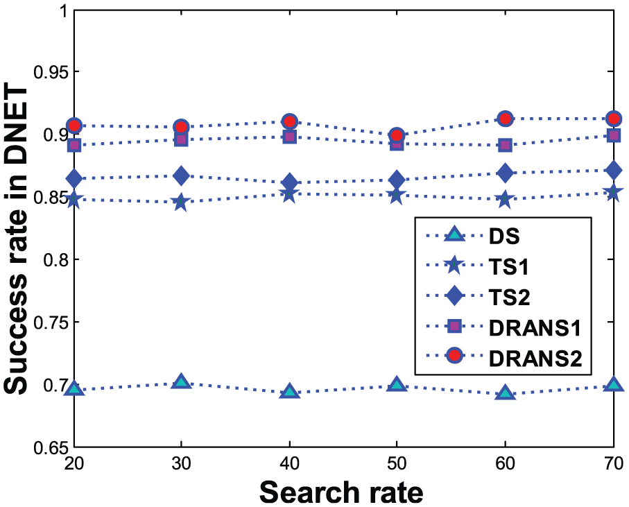
Success rate in DNET.
Through comparing the success rates of DRANS1 and DRANS2 in Figures 8 and 9, it can be seen that DRANS2 has a greater advantage in promoting the success rate, due to it has more forwarding paths and forwarding nodes. Via further observing Figures 8 and 9, we also find that DRANS has a lower success rate in DART than in DNET, which means the success rate of DRANS is influenced by the number of nodes and subareas and it is lower in a great scale DTN than in a small scale one.
Average delay
Figures 10 and 11 show the average delays of different methods under different search rates in DART and DNET, respectively. It can be seen that DRANS has a smaller average delay than all other methods both in DART and DNET, which proves that the node searching strategies in DRANS have higher searching efficiency. In the node searching strategies of DRANS, the SPT and TPT provide a time-related description of node mobility pattern, which can avoid blind searching and reduce node searching time.

Average delay in DART.

Average delay in DNET.
The average delay in DRANS2 is lower than that in DRANS1 both in DART and DNET, which indicates that the increase in the number of forwarding paths and forwarding nodes in DRANS has positive effect on delay reduction. By further comparing the average delay of DRANS in DART and DNET, it can be seen that the larger the network scale, the more the number of nodes and subareas, and the greater average delay of DRANS. Thus, it is better to configure more forwarding paths and forwarding nodes while applying DRANS in a DTN with more nodes and subareas.
Average transmission overhead
Figures 12 and 13 show the average transmission overhead of different methods under different search rates in DART and DNET, respectively. The experimental results show that DRANS spends more average transmission overhead than DS, which can be explained by two reasons: one is that the distribution of SPT and TPT costs more overhead than the dissemination of mobility pattern table in DS, and the other one is that the opportunistic routing strategy needs more overhead. But the average transmission overhead in DRANS is less than that in both TS1 and TS2, which verifies that DRANS has a better advantage in reducing the average transmission overhead than TS1 and TS2.

Average transmission overhead in DART.

Average transmission overhead in DNET.
Due to more forwarding paths and forwarding nodes, the average transmission overhead in DRANS2 is greater than that in DRANS1 both in DART and DNET. In other words, the more the forwarding paths and forwarding nodes, the more the overhead on node searching. Theoretically, DART has more nodes and subareas than DNET, and DART needs to spend much more overhead on the distribution of SPT and TPT and data delivery, which is exactly proved by the experimental results in Figures 12 and 13. Besides, the increase in search rate has less effect on overhead in DART than in DNET, which means the overhead on distribution of SPT and TPT is much more than that on data delivery in a larger scale DTN.
Average memory
Figures 14 and 15 show the average memory usage in different methods under different search rates in DART and DNET, respectively. The experimental results show that the average memory usage in DRANS is more than that in all other methods, which can be explained by the reason that the distribution of SPT and TPT needs more memory than both the encounter information in TSearch and the mobility pattern table in DS.

Average memory in DART.

Average memory usage in DNET.
The average memory in DRANS 2 is almost the same as that in DRANS1 both in DART and DNET, but the average memory of DRANS in DART is much more than that in DNET, which means the number of nodes and subareas has much greater effect on average memory usage in DRANS than the number of forwarding nodes and forwarding paths.
Through observation of all the above simulation results, the characteristics of DRANS can be summarized as follows: (1) due to the SPT and TPT, DRANS provides a more precise and time-related description of node mobility pattern, which can avoid blind node searching and reduce node searching time, thereby contributing to the success rate promotion and transmission delay reduction; (2) but the distribution of SPT and TPT in DRANS consumes more memory usage and transmission overhead, thus, DRANS promotes the success rate and reduces the transmission delay at the expense of more memory usage and transmission overhead; and (3) in addition, with the increase in the network scale, the success rate of DRANS decreases, and conversely, the transmission overhead, delivery delay, and memory usage of DRANS increase.
Conclusion
In this article, DRANS is proposed to promote the success rate and reduce the transmission delay in DTNs, in which each node is required to perform the daily routine analysis and generate the SPT and TPT for providing a more precise and time-related description of node mobility pattern. Each node’s SPT and TPT are distributed to the whole network, for making sure it is traceable for other nodes. On the basis of the SPT and TPT, DRANS further provides two kinds of node searching strategies: the node tracking strategy and the opportunistic routing strategy.
To evaluate the performances of DRANS, we conduct trace-driven experiments and compare DRANS with DSearch and TSearch from four aspects: success rate, transmission delay, average transmission overhead, and average memory usage. The comparison results demonstrate that DRANS has advantages in success rate promotion and transmission delay reduction at the expense of more memory usage and transmission overhead. We also explore the effect of the network scale on the performances of DRANS, and find that with the increase in the network scale, the success rate of DRANS decreases, and conversely, the transmission overhead, delivery delay, and memory usage of DRANS increase.
Our work in this article mainly focuses on the node searching method for small- and medium-scale DTNs. In future work, we will design a hierarchical node searching method for large-scale DTNs, which will explore more nodes’ social properties 25 and absorb studies on nodes’ trajectories, 26 as well as nodes’ energy efficiency. 27
Footnotes
Acknowledgements
The authors would like to appreciate all anonymous reviewers for their insightful comments and constructive suggestions to polish this paper in high quality.
Academic Editor: Sergio Toral
Declaration of conflicting interests
The author(s) declared no potential conflicts of interest with respect to the research, authorship, and/or publication of this article.
Funding
The author(s) disclosed receipt of the following financial support for the research, authorship, and/or publication of this article: The research was supported by the National Natural Science Foundation of China (nos 61602305 and 71690234) and the Shanghai Engineering Research Center Project (no. 14014) jointly.