
Abstract
This article proposes a robust localization algorithm by improving the accuracy of the source position, receiver position, and sound speed using the known position of an object in the sea. The accuracy of those three types of information greatly influences the performance of the target localization in bistatic sonar. Although the locations of the source and receiver can be obtained using the global positioning system, there are still some position errors due to the limitations of global positioning system–based positioning systems and tidal current. In addition, the speed of the sound in the sea changes with temperature. The target estimation error was analyzed mathematically in terms of the mentioned errors. An improved localization is proposed using the accurate positions of objects in the sea, which can compensate for the errors in the source position, receiver position, and sound speed. The proposed algorithm is compared with the conventional algorithm through computer simulations.
Introduction
Sonar systems can be classified into two systems, passive and active, based on the existence of sound sources. Recently, active sonar systems have attracted considerable interest from researchers because submarines are becoming increasingly quieter.1,2 Active sonar can be categorized into monostatic, bistatic, and multistatic sonar according to the number of sources and receivers. Unlike monostatic sonar systems, bistatic and multistatic sonar systems use a spatially separated sound source and receiver, which have an advantage of hiding the receiver position. To obtain the precise location of the target, the source and receiver positions should be known accurately in advance.3–6 In general, the source and receiver positions can be determined using a global positioning system (GPS).6–8 Through the GPS, the source and receiver positions are known but GPS has the errors due to multipaths, interference in ionosphere and troposphere, and so on. 2 And their positions vary with the tidal current as the GPSs are fixed by buoys, and the underwater sensor units are hanged from the buoys by long tethers.
In the conventional literature, the target localization performance was evaluated by considering only the sonar’s geometric configuration.9–18 The performance of the target localization is affected by the following four parameters depending on the accuracy of the information: source and receiver locations, sound velocity, and separation angle. The angle subtended between the source, receiver, and target is called the separation angle. The error in the separation angle is due to the angular measurement accuracy of the receiver. Among the four parameters, the source position, receiver position, and the sound velocity are the parameters that this article is focused on.
The existing errors in the source and receiver locations were taken into account when determining the target localization and sound velocity error.12–18 The accurate target localization was impossible due to those errors, and the impacts of those errors on the target localization were not analyzed. In this article, the impacts of the errors in the source position, receiver position, and the sound velocity are analyzed mathematically in bistatic sonar systems to the target localization. These results can be applied easily to multistatic sonar. An accurate target localization algorithm is proposed by improving the accuracy of the source location, receiver location, and the sound velocity using the known position of an object in the sea. The geographic point of a sea object is assumed to be known by the bottom contour chart. The geographic information gives the specific position of an object at sea that can generate an echo by the transmitted sound signal from the source. The use of one geographic point known in advance gives a solution to improve the target localization.
This article is organized as follows. Section “Bistatic sonar” introduces a brief review of the bistatic sonar system. Section “Target localization by utilizing geographic positions of sea objects” first mathematically analyzes the impacts of the errors of the source position, receiver position, and sound speed to the target localization. An improved target localized algorithm is then proposed. Section “Experimental results” provides the simulation results for performance analysis. Finally, section “Conclusion” concludes the article.
Bistatic sonar
Figure 1 shows the geometric structure of the bistatic sonar.
14
The points S, T, and R denote the source, target, and the receiver, respectively, where
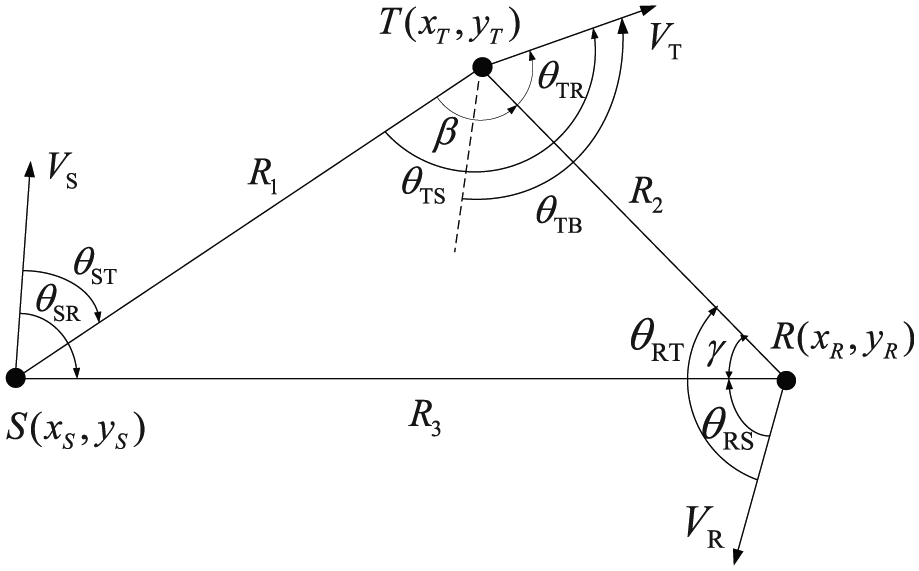
Geometric structure of bistatic sonar. 14
Geometric notation for bistatic sonar.

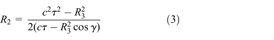
As the source transmits a sound signal, the receiver detects both the direct arrival signals from the source and the target echo. Therefore, the receiver measures the time delay

where

where the separation angle,
After the detection of enemy submarines or torpedoes, tracking work is required. De Theije and Sindt
16
proposed an estimation algorithm of the target speed and heading using the Doppler effect on an active sonar’s ping. The accuracy of target tracking can be improved using the Doppler effect. A signal generated by the source, reflected by the target, and detected by the receiver, will be stretched by an amount that depends on the geometry and the relative motion of the source, target, and receiver. If

where
If the monostatic or bistatic sonar is used, the target speed and direction can be estimated. The relationships of

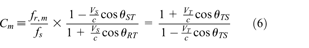
where


From equations (3), (7), and (8), the measurement accuracy of the target information, such as the position, speed, and heading, depends on the accuracy of the pre-defined information. The pre-defined parameters required are the source and receiver positions, sound velocity, and separation angle.
Target localization by utilizing geographic positions of sea objects
In this section, the target localization error is analyzed mathematically in terms of the measurement errors. An improved target localization algorithm is then proposed with the help of the sea object information in a bistatic sonar system. In bistatic sonar, the source and receiver are not collocated, as shown in Figure 1. Therefore, the estimated target position


where ^ denotes a measured value. Through equations (3), (9), and (10), the measured target position contains the errors of the source and receiver positions, sound velocity, and separation angle. The position errors in the source, receiver, and target are as follows 9


where
Using equations (9) and (10), the target localization errors are expressed as follows


Using equations (14) and (15), the target localization variances can be written as


where


To improve the accuracy of the target measurement, the effects of the errors considered should be minimized. This article proposes an algorithm to reduce the target localization errors using a geographic point in the sea. The position of the geographic point must have a fixed location and be known in advance. The geographic information provides the specific position of an underwater geographic point that can generate an echo signal from the source. Using the geographic point, the sound velocity, source and receiver position errors can be minimized. Figure 2 shows the geographic structure of the bistatic sonar with a geographic point
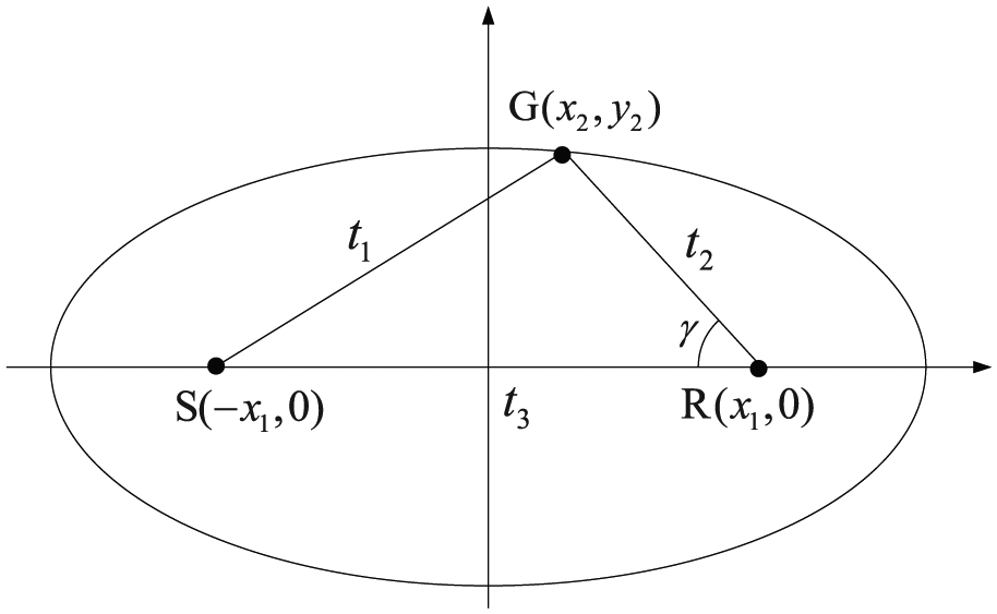
Geometric structure of bistatic sonar using the geographic point.
The wave traveling times


and

where

where

The standard deviation of the timing error is normally small, such as
Experimental results
This section evaluates the proposed algorithm. To confirm the performance of the target localization error, computer simulations were conducted, and the simulation performance was compared with the system without a known geographic point. Table 2 lists the conditions of the simulation. 20
Simulation condition. 20

When the target position is (−2500 m, 2500 m), the target positions are measured by the receiver, as shown in Figure 3, using equations (16) and (17). Monte Carlo simulations were performed 10,000 times considering the target variance. The estimated target positions are represented by dots. For the conventional localization algorithm, the standard deviations

Distributions of the target positions when: (a) the geographic point is not used and (b) the geographic point is used.
To determine the distribution of the target localization error according to the target position, the simulation was conducted in all possible positions of a 5 × 5 km2. The continuous wave (CW) was used as the source. The source and receiver represent the triangle and square. The target position is expressed using the target standard deviations in the x-axis and y-axis to determine the distribution of the measurement error according to the target position. The direct blast, which is the direct signal from the source to the receiver, was applied to masking. 21 Therefore, the target detection is impossible if the target position is between the source and receiver. As the target distance is longer from the source and receiver, the target localization error is also increased, as shown in Figure 4. The target localization error is relatively small, particularly around the outside of the receiver rather than the source. Figure 4(c) and (d) shows that target localization errors are reduced completely by minimizing the errors of the source and receiver and the sound velocity with the geographic point.

Target localization error according to the target position: (a) x-axis measurement error when the geographic point is not used, (b) y-axis measurement error when the geographic point is not used, (c) x-axis measurement error when the geographic point is used, and (d) y-axis measurement error when the geographic point is used.
To verify the numerical results in Figure 4, Figure 5 shows the cumulative distribution function (CDF) of the standard deviation in the target localization error. The standard deviation of the target localization error was reduced using the geographic point. The area with a target standard deviation of less than 40 m was 80% for the proposed algorithm. However, it was 30% for the conventional algorithm. As a result, the accuracy of target detection has been improved.

CDF of the measurement error.
Until now, a point object was considered as the sea object. However, the geographic point has a volume so the geographic point can have positional errors due to the size of the object. The CDFs of standard deviation for the length of geographic points are shown in Figure 6. The proposed algorithm has an improved localization performance over the conventional algorithm when the object’s length is 20 m. However, the performance can be worsened with an object with length 30 m. From this point, if the length of the geographic point is less than 20 m, the proposed algorithm shows better performance than the conventional algorithm.
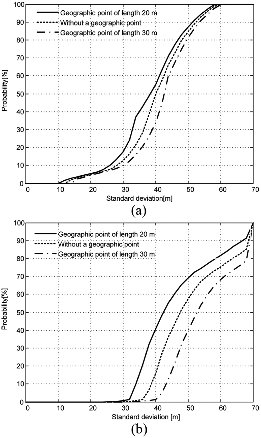
CDF of the measurement error according to the geographic point size: (a) measurement error in x-axis and (b) measurement error in y-axis.
Conclusion
Owing to the source and receiver position errors, there are measurement errors in the separation angle error and sound speed. Therefore, the target localization error is dependent on those measurement errors. This article analyzed those error effects in the target localization mathematically and proposed how to minimize the measurement errors in the source and receiver positions and sound speed. The experimental results showed that the proposed target localization using the known position of an object improves on the localization performance by 50% over the conventional algorithm. And the analysis of the localization error of GPS has contributed the localization techniques in wireless sensor networks. In practical environments, the number of referenced objects is more than one in this article. The impact should be analyzed to adopt the proposed algorithm in the practical system.
Footnotes
Appendix 1
In this appendix, each variance expressed in equations (16) and (17) are analyzed. Equations (1) and (2) were combined to eliminate
The errors in
where
Using equations (27) and (28),
Using equations (27) and (29),
Using equations (27) and (30),
From equations (28) and (29),
Using equations (28) and (30),
Using equations (28) and (30),
From equations (26) and (28),
Using equation (55), the variance of
The variance of
Therefore, equations (16) and (17) can be calculated using equations (25)–(58).
Academic Editor: Minglu Jin
Declaration of conflicting interests
The author(s) declared no potential conflicts of interest with respect to the research, authorship, and/or publication of this article.
Funding
The author(s) disclosed receipt of the following financial support for the research, authorship, and/or publication of this article: This work was supported by the Agency for Defense Development under the contract UD160004DD.