Sage Journals: Discover world-class research

Abstract

This paper presents a vision-based, computationally efficient method for simultaneous robot motion estimation and dynamic target tracking while operating in GPS-denied unknown or uncertain environments. While numerous vision-based approaches are able to achieve simultaneous ego-motion estimation along with detection and tracking of moving objects, many of them require performing a bundle adjustment optimization, which involves the estimation of the 3D points observed in the process. One of the main concerns in robotics applications is the computational effort required to sustain extended operation. Considering applications for which the primary interest is highly accurate online navigation rather than mapping, the number of involved variables can be considerably reduced by avoiding the explicit 3D structure reconstruction and consequently save processing time. We take advantage of the light bundle adjustment method, which allows for ego-motion calculation without the need for 3D points online reconstruction, and thus, to significantly reduce computational time compared to bundle adjustment. The proposed method integrates the target tracking problem into the light bundle adjustment framework, yielding a simultaneous ego-motion estimation and tracking process, in which the target is the only explicitly online reconstructed 3D point. Our approach is compared to bundle adjustment with target tracking in terms of accuracy and computational complexity, using simulated aerial scenarios and real-imagery experiments.

Keywords

Simultaneous localization and mapping bundle adjustment navigation computer vision target tracking

Introduction

Ego-motion estimation and target tracking are core capabilities required in a wide range of applications. While motion estimation is essential to numerous robotics tasks such as autonomous navigation^1,2,3,4 and augmented reality,^5,6 target tracking has been essential, amongst others, for video surveillance⁷ and for military purposes.⁸ Although researched for decades, target tracking methods have mostly assumed a known or highly predictable sensor location. Recent robotics applications such as autonomous aerial urban surveillance⁹ or indoor navigation require the ability to track dynamic objects from platforms while moving in unknown or uncertain environments. The ability to simultaneously solve the ego-motion and target tracking problems becomes therefore an important task. Furthermore, attention has grown for cases in which external localization systems (e.g. GPS) are unavailable and the estimation process must be performed using on-board sensors only. In particular, the capability to perform those tasks based on vision sensors has become of great interest in the past two decades, mostly thanks to the ever-growing advantages these sensors present.¹⁰

Vision-based ego-motion estimation is typically performed as part of a process known as bundle adjustment (BA) in computer vision, or simultaneous localization and mapping (SLAM) in robotics, where the differences between the actual and the predicted image observations are minimized. Therefore, the combined process of SLAM and tracking of a moving object usually involves an optimization over the camera’s motion states, the target’s navigation states, and the observed structure (3D landmarks). This optimization is performed incrementally as new information and variables are added to the process, constantly increasing the computational complexity of the problem. One of the main challenges in extended operation is thus keeping computational efforts to a minimum despite the growing number of variables. However, many robotics applications do not require actual online mapping of the environment. Avoiding this expensive task would therefore be beneficial in terms of processing time.

This work presents a computationally efficient approach for simultaneous camera ego-motion estimation and target tracking, while operating in unknown or uncertain GPS-deprived environments. Our focus lies on robotic applications for which online 3D structure reconstruction is of no interest, although recovering the latter offline from optimized camera poses is always possible.¹¹ We propose to take advantage of the recently developed incremental light bundle adjustment (iLBA)^11–13 framework, which uses multi-view constraints to algebraically eliminate the (static) 3D points from the optimization, therefore allowing the dynamic target to become the only explicitly reconstructed 3D point in the process. The reduced number of variables involved in the optimization allows therefore for substantial savings in computational efforts. Incremental smoothing and mapping (iSAM)¹⁴ technique is applied to re-use calculations, allowing to further reduce running time, in a similar fashion to the static-scene-oriented iLBA approach. We demonstrate, using simulations on synthetic datasets and real-imagery experiments, that while our methods provide similar levels of accuracy to full BA with target tracking, they compare favorably in terms of computational complexity.

The simultaneous ego-motion and dynamic object tracking relate to numerous works on SLAM and target tracking, both individually and combined. Early approaches used the extended Kalman filter (EKF) to solve the SLAM problem^15,16 but were eventually overtaken by other techniques due to their quadratic computational complexity, which limits them to relatively small environments or to relatively small state vectors. Numerous SLAM methods have been proposed to overcome computational complexity, for example, by exploiting the sparsity of the involved matrices,^17,18 or by approximating the full problem with a reduced non-linear system.¹⁹ A more recent technique, used in the frame of this work, performs incremental smoothing¹⁴ to recover the solution while recalculating only part of the variables at each optimization step and allows for a significant reduction of the computational cost. Still, full BA methods involve the reconstruction of the 3D observed structure, increasing unnecessarily the number of estimated variables in cases online mapping is of no interest. Several “structure-less” BA approaches have been developed, where the optimization satisfies constraints which do not involve 3D structure reconstruction. Rodríguez et al.²⁰ use epipolar constraints between pairs of views, while Steffen et al.²¹ utilize trifocal tensor constraints. The recently developed LBA method,¹² used in this work, applies two kinds of multi-view constraints: the two-view and three-view constraints. Pose-SLAM techniques^22,23 avoid explicit mapping by maintaining the camera trajectory as a sparse graph of relative pose constraints, which are calculated using the landmarks in a separate process. In contrast to standard Pose-SLAM, LBA formulates multi-view geometry constraints for each feature match, thereby avoiding to rely on the uncertainty of the abovementioned separate process.

The target tracking problem, referred more generally as detection and tracking of moving objects (DTMO)²⁴ in the robotics literature, has been extensively studied for several decades.^25,26 The combined SLAM and DTMO problem, which is assessed in our work, has attracted considerable attention in the recent years, mostly in order to improve SLAM accuracy, which can be greatly degraded by the presence of dynamic objects in the environment, if the latter is considered as static.²⁷ The first mathematical framework to the combined process of simultaneous localization, mapping, and moving object tracking (SLAMMOT) was presented by Wang,²⁸ where the problem is decomposed into two separate estimators, one for the SLAM problem given the static landmarks and another for the tracking problem. Occupancy grid-based approaches were proposed later by Vu et al.²⁹ and Vu,¹ where SLAM was solved by calculating the maximum likelihood of occupancy grid maps. Ortega³⁰ introduced a geometric and probabilistic approach to the vision-based SLAMMOT problem, providing a comparison between the different kinds of optimization methods, while Hahnel et al.³¹ used sampled-based joint probabilistic data association filter to track people and occupancy grids for static landmarks. An extensive overview of the literature concerning SLAM and DTMO is presented in Pancham et al.³²

The rest of this paper is structured as follows: First, we formulate the simultaneous ego-motion estimation and moving object tracking problem. Next, we review the LBA method, which is extended to address the mentioned problem. Then, we present experimental results, comparing our method with full BA in terms of computation time and accuracy. Finally, we conclude and share thoughts about further possible developments.

Problem formulation and notations

We consider a scenario where a monocular camera mounted on a mobile robot is tracking a dynamic target while operating in a GPS-deprived unknown environment.

The BA problem

The process of determining the camera poses and the stationary 3D structure given measurements is called BA or SLAM. Let x_k represent the camera pose (i.e. 6DOF position and orientation) at time step t_k, and denote all such states up to that time by $X_{k} ≐ {\begin{matrix} x_{0} & \dots & x_{k} \end{matrix}}$ . We also use $L_{k} ≐ {\begin{matrix} l_{1} & \dots & l_{n} \end{matrix}}$ and $Z_{k} ≐ {\begin{matrix} z_{0} & \dots & z_{k} \end{matrix}}$ to represent, respectively, all the n landmarks observed by time t_k, and the corresponding sensor observations. Here, for each time index $i \in [0, k]$ , z_i corresponds to all image observations obtained at time t_i. In particular, we use the notation $z_{i}^{j}$ to denote an observation of the jth landmark at time t_i.

Using probabilistic representation, the BA problem can be expressed by the joint pdf

P (X_{k}, L_{k} | Z_{k})

(1)

Using Bayes’ rule, the general recursive Bayesian formula for BA can be derived as³³

P (X_{k}, L_{k} | Z_{k}) \propto p r i o r s \cdot \prod_{i = 1}^{k} \prod_{j \in M_{i}} p (z_{i}^{j} | x_{i}, l_{j})

(2)

where

M_{i}

is the set of landmarks observed at time index i and priors represent prior information on the estimated variables.

Considering a standard pinhole camera, the corresponding observation model can be defined as³⁴

z_{i}^{j} = p r o j (x_{i}, l_{j}) + v_{i j}

(3)

where

p r o j (\cdot)

is the projection operator³⁴ and

v_{i j} \sim N (0, Σ_{v})

is a zero-mean white noise with measurement covariance Σ _v . Under Gaussian distribution assumption, the likelihood of the perception measurement can be expressed as

p (z | x, l) ≐ \frac{1}{\sqrt{| 2 π Σ_{v} |}} \exp (- \frac{1}{2} | | z - p r o j (x, l) | |_{Σ_{v}}^{2})

(4)

where

{‖ a ‖}_{Σ}^{2} ≐ a^{T} Σ^{- 1} a

is the squared Mahalanobis distance with the measurement covariance matrix Σ. We assume camera calibration is known; otherwise, the uncertain calibration parameters could be incorporated into the optimization framework as well.

Solving the BA problem would therefore consist in calculating the maximum a posteriori estimate over the joint pdf, defined as

X_{k}^{*}, L_{k}^{*} = \underset{X_{k}, L_{k}}{arg max} P (X_{k}, L_{k} | Z_{k})

(5)

Due to the monotonic characteristics of the logarithmic function, calculating the MAP estimate $X_{k}^{*}, L_{k}^{*}$ becomes equivalent to minimizing the negative log-likelihood of the BA pdf 1

X_{k}^{*}, L_{k}^{*} = \underset{X_{k}, L_{k}}{arg min} - \log P (X_{k}, L_{k} | Z_{k})

(6)

This leads to a non-linear least-squares optimization, where the cost function

J_{B A} (X_{k}, L_{k}) = \sum_{i} \sum_{j \in M_{i}} | | z_{i}^{j} - p r o j (x_{i}, l_{j}) | |_{Σ}^{2}

(7)

is to be minimized. Note that, to avoid clutter, the prior terms are not explicitly shown in equation (7).

BA and target tracking

We investigate scenarios in which a dynamic target is tracked by the camera. Based on the camera’s observations of the target, we seek to estimate its trajectory and velocity over time. We assume the target moves randomly; however, its motion is assumed to follow a known stochastic kinematic model (e.g. constant velocity or constant acceleration).

Let y_k represent the target state at time step t_k, defined generally as

y_{k} ≐ {[y_{T_{k}} d_{T_{k}}]}^{T} = {[x_{T_{k}}, y_{T_{k}}, z_{T_{k}}, {\dot{x}}_{T_{k}}, {\dot{y}}_{T_{k}}, {\dot{z}}_{T_{k}}, …]}^{T}

(8)

where

y_{T_{k}}

denotes the target’s tri-dimensional position and

d_{T_{k}}

its higher order time derivatives required to accommodate the assumed motion model. In the frame of this work, we focus on the target’s position and velocity. y_k is therefore a six element vector defined as

y_{k} = [\begin{matrix} y_{T_{k}} \\ {\dot{y}}_{T_{k}} \end{matrix}] \in R^{6 \times 1}

(9)

We denote $Y_{k} ≐ {\begin{matrix} y_{0} & \dots & y_{k} \end{matrix}}$ the set of all target’s states up to time step t_k.

Assuming a known Markovian motion model for the target, which likelihood is represented by $p (y_{i} | y_{i - 1})$ , we define a joint pdf for the random variables involved in the considered problem, given all information thus far, as

\begin{array}{l} P (X_{k}, Y_{k}, L_{k} | Z_{k}) \propto p r i o r s \cdot \\ \prod_{i = 1}^{k} (p (y_{i} | y_{i - 1}) p (z_{i}^{y_{i}} | x_{i}, y_{i}) \prod_{j \in M_{i}} p (z_{i}^{j} | x_{i}, l_{j})) \end{array}

(10)

where

z_{i}^{y_{i}}

denotes the observation of the target by the ith camera and

p (z_{i}^{y_{i}} | x_{i}, y_{i})

refers to the observation model described in equation (3).

M_{i}

is the set of landmarks observed at time index i and we consider

p r i o r s = p (x_{0}) p (y_{0})

as given information.

In this work, as in many robotics applications, we consider a constant velocity model,³⁵ characterized by the equation

\ddot{y} (t) = \tilde{w} (t)

(11)

where

\tilde{w} (t)

is a continuous time zero-mean white noise representing the slight velocity changes from its actual value.

The target state linear continuous propagation is generally noted as $\dot{y} (t) = A y (t) + D w (t)$ , where $A = [\begin{matrix} 0 & 1 \\ 0 & 0 \end{matrix}]$ and $D = [\begin{matrix} 0 \\ 1 \end{matrix}]$ , or under its discrete form

y_{k + 1} = Φ_{k} y_{k} + G_{k} w_{k}

(12)

where G_k is the process noise Jacobian defined as

G_{k} = [\begin{matrix} 0 \\ 1 \end{matrix}] \in R^{6 \times 3}

and

Φ_{k}

is the state transition matrix and is defined as

Φ_{k} = [\begin{matrix} 1 & △ t \\ 0 & 1 \end{matrix}] \in R^{6 \times 6}

with

△ t ≐ t_{k + 1} - t_{k}

. The discrete-time process noise

w_{k} \sim N (0, Σ_{w})

relates to the continuous-time one as

w_{k} = \int_{0}^{Δ t} e^{A (Δ t - τ)} D \tilde{w} (k Δ t + τ) d τ

. Under Gaussian distribution assumption, the motion model likelihood is therefore expressed

p (y_{k + 1} | y_{k}) ≐ \frac{1}{\sqrt{| 2 π Σ_{m m} |}} \exp (- \frac{1}{2} | | y_{k + 1} - Φ_{k} y_{k} | |_{Σ_{m m}}^{2})

(13)

where

Σ_{m m} ≐ G Σ_{w} G^{T}

Finally, solving the combined BA and target state estimation process consists in calculating the MAP estimate over the joint pdf from equation (10)

X_{k}^{*}, Y_{k}^{*}, L_{k}^{*} = \underset{X_{k}, Y_{k}, L_{k}}{arg max} P (X_{k}, Y_{k}, L_{k} | Z_{k})

(14)

Factor graph representation

As mentioned earlier, the factorization of the joint pdf described in equation (10) can be represented using a factor graph,³⁶ which will be used later to efficiently solve the optimization problem using incremental inference. Using the same observation (equation (3)) and motion (equation (12)) models, this pdf is expressed in factor graph notation as

\begin{array}{l} P (X_{k}, Y_{k}, L_{k} | Z_{k}) \propto p r i o r s \\ \times \prod_{i = 1}^{k} (​ f_{m m} (y_{i}, y_{i - 1}) f_{p r o j} (x_{i}, y_{i}) \prod_{j \in M_{i}} f_{p r o j} (x_{i}, l_{j})) \end{array}

(15)

An illustration expressing the above factorization for a small example is shown in Figure 1. The corresponding factors in equation (15) are straightforwardly defined as follows: The factor $f_{m m} (y_{i}, y_{i - 1})$ corresponds to the target motion model and, referring to equations (12) and (13), is defined as

f_{m m} (y_{i}, y_{i - 1}) ≐ \exp (- \frac{1}{2} | | y_{i} - Φ_{i - 1} y_{i - 1} | |_{Σ_{m m}}^{2})

(16)

Figure 1.

Factor graph representing a factorization of the joint pdf for bundle adjustment with single target tracking.

The projection factors $f_{p r o j} (x_{i}, l_{j})$ and $f_{p r o j} (x_{i}, y_{i})$ correspond to the landmarks and target observation models; these factors are defined, respectively, as

f_{p r o j} (x_{i}, l_{j}) ≐ \exp (- \frac{1}{2} | | z_{i}^{j} - p r o j (x_{i}, l_{j}) | |_{Σ_{v}}^{2})

(17)

f_{p r o j} (x_{i}, y_{i}) ≐ \exp (- \frac{1}{2} | | z_{i}^{y_{i}} - p r o j (x_{i}, y_{i}) | |_{Σ_{v}}^{2})

(18)

Similarly to the previous section, the MAP estimate is defined as

X_{k}^{*}, Y_{k}^{*}, L_{k}^{*} = \underset{X_{k}, Y_{k}, L_{k}}{arg max} P (X_{k}, Y_{k}, L_{k} | Z_{k})

(19)

and can be efficiently calculated by exploiting the inherent sparse structure of the problem while re-using calculations.

This corresponds to the state of the art where inference is performed over camera poses, landmarks, and target states. Yet, when the primary focus is navigation rather than mapping, explicit estimation of the observed landmarks in an online process is not actually required. Conceptually, estimating only the camera poses and the dynamic target (but not the landmarks) involves less variables to optimize and could be attractive from a computational point of view. In this work, we develop an approach based on this idea.

LBA and dynamic target tracking

BA is a non-linear iterative optimization framework typically applied for estimating camera poses and observed landmarks. In this section, we integrate target tracking to a structure-less BA technique called light bundle adjustment (LBA).¹³ First, we formulate the LBA equations while considering a static scene. These equations are then extended to incorporate the dynamic target tracking problem.

Using factor graph notations, the joint pdf $P (X_{k}, L_{k} | Z_{k})$ , which corresponds to the static problem, can be factorized similarly to equation (15) as

P (X_{k}, L_{k} | Z_{k}) \propto p r i o r s \cdot \prod_{i = 1}^{k} (\prod_{j \in M_{i}} f_{p r o j} (x_{i}, l_{j}))

(20)

where

p r i o r s = p (x_{0}) p (y_{0})

represents the prior information on the camera and target states.

As mentioned, this works considers robotics applications in which the online reconstruction of the 3D structure is of no interest. One way to avoid explicit estimation of the landmarks in the solution is by marginalizing out the latter from the joint pdf as in

P (X_{k} | Z_{k}) = \int P (X_{k}, L_{k} | Z_{k}) d L_{k}

(21)

However, this involves a series of calculations which, in the case of online operation, could be penalizing: First, performing the exact marginalization would initially require to solve the full BA problem, including landmarks, before applying a Gaussian approximation to compute the marginal. Secondly, marginalization in the information form involves the expensive calculation of the Schur complement over the variables we wish to keep.²² Moreover, marginalization introduces fill-in, destroying the sparsity of the information matrix.

In contrast, structure-less BA methods approximate the BA cost function, allowing for estimation of the camera poses without involving the reconstruction of the 3D structure.^20,21 In this work, we use the recently developed LBA approach,^11,12 which algebraically eliminates the landmarks from the optimization, using multi-view constraints and in particular, three-view constraints.

LBA

LBA allows for reduction of the number of variables involved in the optimization compared to standard BA. By algebraically eliminating the landmarks from the problem, the optimization can be performed over the camera poses only. The key idea is to use geometrical constraints relating three views from which the same landmark is observed.

Considering a set of three overlapping poses k, l and m from which a common landmark is observed, it is possible to derive constraints that relate the three poses while eliminating the landmark.³⁷ These constraints can be formulated as two two-view constraints $g_{2 v}$ between two pairs of poses (e.g. (k, l) and (l, m)) and one three-view constraint $g_{3 v}$ between the three involved poses.^37,38 Conceptually, the two-view constraint is equivalent to the epipolar constraint,³⁴ while the three-view constraint relates between the scales of the two translations $t_{k \to l}$ and $t_{l \to m}$ . Writing down the appropriate projection equations, we get

g_{2 v} (x_{k}, x_{l}, z_{k}, z_{l}) = q_{k} \cdot (t_{k \to l} \times q_{l})

(22)

g_{2 v} (x_{l}, x_{m}, z_{l}, z_{m}) = q_{l} \cdot (t_{l \to m} \times q_{m})

(23)

\begin{array}{l} g_{3 v} (x_{k}, x_{l}, x_{m}, z_{k}, z_{l}, z_{m}) \\ = (q_{l} \times q_{k}) \cdot (q_{m} \times t_{l \to m}) - (q_{k} \times t_{k \to l}) \cdot (q_{m} \times q_{l}) \end{array}

(24)

$q_{i} ≐ R_{i}^{T} K_{i}^{- 1} z$ for the ith view and image observation z, where K_i is the calibration matrix, R_i represents the rotation matrix from some reference frame to the ith view, and $t_{i \to j}$ denotes the translation vector from view i to view j, expressed in the global frame.

The resulting probability distribution $P_{L B A} (X | Z)$ can thus be factorized as

P_{L B A} (X | Z) \propto \prod_{i = 1}^{N_{h}} f_{2 v / 3 v} (X_{i})

(25)

where

f_{2 v / 3 v}

represents the involved two- and three-view factors and X_i is the relevant subset of camera poses. Referring to equations (22) to (24), under Gaussian distribution assumption,

f_{2 v}

and

f_{3 v}

are defined as

f_{2 v} (x_{k}, x_{l}) ≐ \exp (- \frac{1}{2} | | g_{2 v} (x_{k}, x_{l}, z_{k}, z_{l}) | |_{Σ_{2 v}}^{2})

(26)

and

\begin{array}{l} f_{3 v} (x_{k}, x_{l}, x_{m}) \\ ≐ \exp (- \frac{1}{2} | | g_{3 v} (x_{k}, x_{l}, x_{m}, z_{k}, z_{l}, z_{m}) | |_{Σ_{3 v}}^{2}) \end{array}

(27)

which correspond to the likelihoods of the two- and three-views constraints involving x_k and x_l in equation (26) and involving x_k, x_l and x_m in equation (27). The covariances

Σ_{2 v}

and

Σ_{3 v}

are defined as

\begin{array}{l} Σ_{2 v} ≐ (\nabla_{z_{k}, z_{l}} g_{2 v}) Σ {(\nabla_{z_{k}, z_{l}} g_{2 v})}^{T}, \\ Σ_{3 v} ≐ (\nabla_{z_{k}, z_{l}, z_{m}} g_{3 v}) Σ {(\nabla_{z_{k}, z_{l}, z_{m}} g_{3 v})}^{T} \end{array}

(28)

Figure 2 shows a comparison between the factor graph representation of LBA and standard BA for a small example.

Figure 2.

Factor graph representation for a small example including three views x_k, x_l, x_m. (a) The BA problem, where the three views are related to the landmark l with projection factors. (b) The LBA problem, where the landmark l has been eliminated, and the three views are related by two- and three-view constraints.

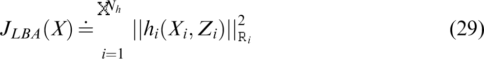
Therefore, rather than optimizing the cost function 7, that involves the camera and landmark states, the optimization is performed on the cost function¹¹

J_{L B A} (X) ≐ \sum_{i = 1}^{N_{h}} | | h_{i} (X_{i}, Z_{i}) | |_{Σ_{i}}^{2}

(29)

where

h_{i} \in {g_{2 v}, g_{3 v}}

represents a single two- or three-view constraint involving the set of poses X_i and the set of image observations Z_i, N_h being the number of resulting constraints.

Practically, when a landmark is observed by a new view x_k and some earlier views x_l and x_m, a single two-view (between x_k and one of the two other views) and a single three-view constraint are added (between the three views). The reason for not adding the second two-view constraint (between views x_l and x_m) is that this constraint was already added when processing these past views. In case a landmark is observed by only two views, we add a single two-view constraint.

LBA and dynamic target tracking

In this section, we integrate dynamic target tracking into the LBA framework. As will be shown, the resulting approach provides comparable accuracy for both target tracking and camera pose estimation while significantly reducing running time, compared to an equivalent BA approach.

The idea behind the proposed method is to incorporate the target tracking problem into the LBA framework in order to yield a proxy for the joint pdf $P (X_{k}, Y_{k} | Z_{k})$ which involves significantly less variables than the joint pdf $P (X_{k}, Y_{k}, L_{k} | Z_{k})$ , while somewhat avoiding the expensive calculations involved in the marginalization process.¹¹ Indeed, if $X_{k} \in R^{M_{k} \times 1}$ , $Y_{k} \in R^{N_{k} \times 1}$ and $L_{k} \in R^{O_{k} \times 1}$ , then the amount of variables involved in the optimization is decreased form $M_{k} + N_{k} + O_{k}$ to $M_{k} + N_{k}$ only, which would reduce computational complexity (we note that $O_{k} ≫ M_{k}$ and $O_{k} ≫ N_{k}$ ).

We integrate the factors $f_{2 v / 3 v}$ corresponding to the camera poses described in equations (26) and (27) with the target tracking-related factors f_mm and f_proj defined in equations (16) and (18) to yield the joint pdf $P (X_{k}, Y_{k} | Z_{k})$ over the relevant states only. The target becomes, therefore, the only 3D point to be estimated in the process

\begin{array}{l} P (X_{k}, Y_{k} | Z_{k}) \propto p r i o r s \\ \times \prod_{i = 1}^{k - 1} (f_{m m} (y_{i}, y_{i - 1}) f_{p r o j} (x_{i}, y_{i}) \prod_{j = 1}^{N} f_{2 v / 3 v} (X_{j})) \end{array}

(30)

where, similar to equation (15),

p r i o r s = p (x_{0}) p (y_{0})

represents the prior information and X_j is the relevant subset of views for the ith frame.

Solving the localization and target tracking problem then corresponds to estimating the MAP

X_{k}^{*}, Y_{k}^{*} = \underset{X_{k}, Y_{k}}{arg max} P (X_{k}, Y_{k} | Z_{k})

(31)

which is equivalent to minimizing the cost function

\begin{matrix} J (X_{k}, Y_{k}) = | | x_{0} - {\hat{x}}_{0} | |_{Σ_{x}}^{2} + | | y_{0} - {\hat{y}}_{0} | |_{Σ_{y}}^{2} \\ + \sum_{i = 1}^{k} {(| | y_{i} - Φ_{i} y_{i - 1} | |}_{Σ_{m m}}^{2} + | | z_{i}^{y_{i}} \\ - p r o j (x_{i}, y_{i}) | |_{Σ_{v}}^{2} \\ + \sum_{j}^{N_{h}} | | h_{j} (X_{j}, Z_{j}) | |_{Σ_{j}}^{2}) \end{matrix}

(32)

An illustration expressing the above factorization for the same example as in Figure 1 is shown in Figure 3.

Figure 3.

Factor graph representing a factorization of the joint pdf for LBA and target tracking.

LBA and multi-target tracking

The considered problem can be straightforwardly extended to multi-target tracking by integrating the additional targets into the formulation from equation (30). Considering n targets, the corresponding joint pdf can be written

\begin{array}{l} P (X_{k}, {\bar{Y}}_{k} | Z_{k}) \propto p r i o r s \\ \times \prod_{i = 1}^{k - 1} (\prod_{l = 1}^{n} f_{m m} (y_{i}^{l}, y_{i - 1}^{l}) \prod_{p \in T_{i}} f_{p r o j} (x_{i}, y_{i}^{p}) \prod_{j = 1}^{N} f_{2 v / 3 v} (X_{j})) \end{array}

(33)

where

{\bar{Y}}_{k} = {Y_{k}^{1}, Y_{k}^{2}, …, Y_{k}^{n}}

is the set of all targets’ states up to time-step t_k and

Y_{k}^{n}

refers to the states of the nth target up to time-step t_k. We denote

T_{i}

the set of targets observed at time-step t_i. Here, we assume the identification of the targets that leave and re-enter the camera’s field of view as given. Solving this data-association problem is a challenging task by itself and is outside the scope of this work.

Incremental smoothing

Solving the abovementioned non-linear least square problems is achievable using several optimization methods. Online operation requires this task to be performed efficiently, and therefore, cost-efficient techniques were implemented in this work.

Batch optimization performs factorization of the Jacobian matrix A from scratch each time new variables are added to the problem. In contrast, incremental smoothing updates the problem as new measurements and variables arrive, by directly updating the square root information matrix R and recalculating only the matrix entries that actually change.³⁹ Furthermore, instead of performing batch re-ordering, eliminating the corresponding factor graph into a Bayes tree¹⁴ allows for incremental variable ordering, which keeps the R matrix sparsity at a relatively constant level. Additionally, rather than fully re-linearizing the whole set of variables at a determined point in time, iSAM2 performs fluid re-linearization, which triggers re-linearization of a variable only when the deviation between its current estimate and the linearization point is larger than a defined threshold, set heuristically or as part of a “tuning” process.

Results

We demonstrate the benefits of the proposed method with simulations performed on synthetic datasets and with real-imagery experiments. Experiments were performed considering a downward-facing camera mounted on a flying vehicle, which tracks a single target, for the sake of simplicity. For each scenario, target tracking and ego-pose estimation using LBA and full BA are compared in terms of accuracy and processing time. All experiments were run on an Intel i7-4720HQ quadcore processor with 2.6 GHz clock rate and 8GB of RAM. The methods used for comparison were implemented using the GTSAM library (https://research.cc.gatech.edu/borg/download).

Experimental evaluation with synthetic datasets

A series of simulations were performed on synthetic datasets in order to compare our method with full BA technique and to demonstrate its capability in terms of computational performance and estimation accuracy for both camera and target states. We present two types of studies: A statistical performance study on an approximately 3-km long aerial scenario (Figure 4), and a case study in a larger aerial scenario (Figure 6(a)). In both cases, the downward-facing camera operates in GPS-denied environments and occasionally re-visits previously explored locations, providing occasional loop-closure measurements. The priors $p (x_{0})$ and $p (y_{0})$ are Gaussians with means equal to their initial values, and with $σ = 2 [m]$ standard deviation. The measurement model assumes an image noise $σ = 0.5 [pix]$ . The continuous-time system is discretized with time-step $△ t = 3 [s]$ . Regarding target motion, we use the constant velocity model and assume a zero-mean, white Gaussian noise $σ = {[30, 30, 0.001]}^{T} [m / s]$ . Here, we constrained the noise on the z axis to prevent divergence, both with LBA and BA, which use data only from a single monocular camera. Addressing this issue would probably require additional information or constraints on the target motion (multi-robot setup, additional sensors, geometric constraints, etc.).

Figure 4.

Scenario used for statistical study. Camera and target trajectories are shown in red and blue, respectively. At this scale, ground truth and estimated trajectories are indistinguishable (see Figure 5).

Statistical simulation results

A performance comparison between the proposed method and BA with target tracking is presented in a 45-run Monte-Carlo study. The scenario used in this simulation, shown in Figure 4, contains 52 frames, gathered over ∼160 s. Loop-closures can be noticed around views 20 and 38. The simulated target takes a similar course on the ground and for the sake of simplicity, stays in the camera’s field of view throughout the process. The comparisons presented in Figure 5(a) to (c) are given in terms of root-mean-square error (RMSE), calculated over the norms of the error vectors. All results refer to incremental estimations, i.e. at each time t_k performance is evaluated given Z_k, which is in particular important for online navigation.

Figure 5.

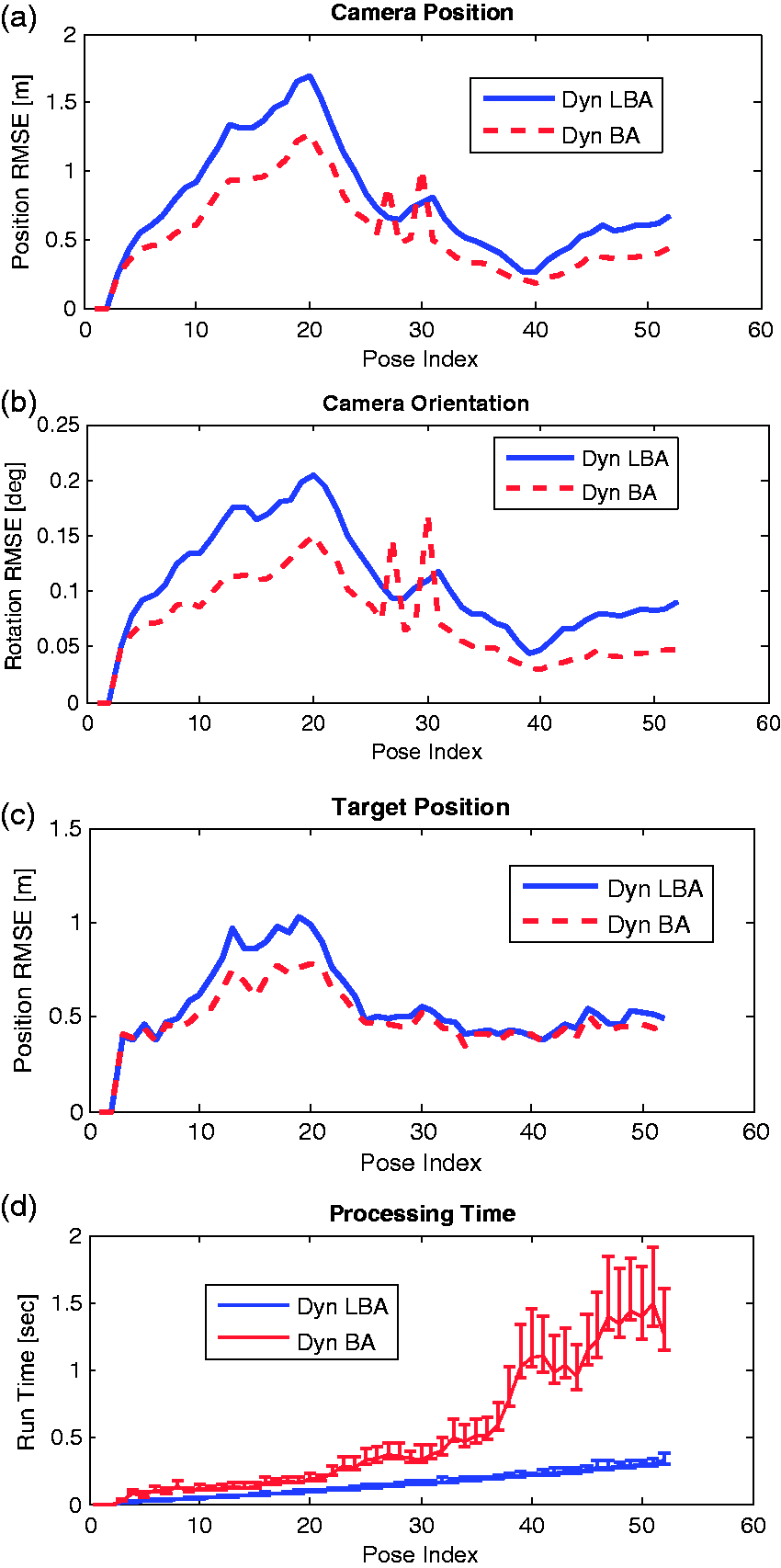
Monte-Carlo study results comparing between the proposed method and full BA with target tracking (a) camera position RMSE; (b) camera orientation RMSE (including close-up); (c) target position RMSE; (d) running time average with lower and upper boundaries.

Figure 5(a) and (b) describes the camera incremental position and orientation errors and Figure 5(c) shows the target position error. We observe similar levels of accuracy with the two techniques. The camera pose and target trajectory errors are bounded, with clear negative trend in both the camera and target position errors around view 20, upon loop closure. We note that, in this case, the navigation is performed relatively to the camera’s and target’s initial positions. Those were initialized from their ground truth values, causing initial errors to be zero for all the estimated states.

Figure 5(d) shows statistics over running time between the proposed method and full BA with target tracking. For BA, a distinct increase in computational time can be observed at view 38, where a loop closure occurs. While one can already observe a significant difference in running time between the two methods in favor of LBA, we confirm this observation further in a larger scenario and with real imagery experiments in the next sections.

Large scenario

The large scenario, shown in Figure 6(a), simulates an approximately 14.5-km-long aerial path and involves a series of loop closures, resulting in variables recalculation during optimization. The target takes a different course on the ground (as shown in Figure 6(b)), which causes losses of target sight for approximately a seventh of the frames. In these cases, only the motion model factor is taken into consideration.

Figure 6.

(a) Estimated camera (red) and target (blue) trajectories for the large synthetic scenario with 24,500 observed landmarks (shown in black). (b) Top view of the target and camera estimated trajectories for the large-scale synthetic scenario. At this scale, ground truth and estimated trajectories are indistinguishable (see Figure 7).

The obtained average camera position incremental errors for LBA and BA are 1.27 and 0.51 m, respectively, with a maximum error of 5.11 and 2.33 m. While the accuracy levels are similar, one can easily notice the difference in running time. Loop closures have a high impact on BA running time due to the landmark re-elimination and re-linearization they trigger; this process is avoided with LBA. It results in an average processing time of 3.3 s for LBA with target tracking, versus 22.2 s for BA method. The obtained overall processing time for the same scenario is 809 s for the proposed method, versus 5329 s with BA.

Since we are interested to assess the similarity in terms of accuracies between the two techniques, we show in Figure 7(a) to 7(c) the relative errors between LBA and BA methods, meaning the difference between the estimation errors using both methods. Then, a comparison of the processing time is shown in Figure 7(d).

Figure 7.

Incremental relative errors of LBA method with respect to BA method for the (a) camera position, (b) camera orientation, (c) target position, in the large-scale synthetic scenario. (d) a comparison of the processing times per frame.

Experimental evaluation with real-imagery datasets

Further evaluations were performed through real-world experiments conducted at the Autonomous Navigation and Perception Lab (ANPL). Similarly to the synthetic dataset evaluation, these experiments involve a downward-facing camera which performed an aerial pattern while tracking a dynamic target moving on the ground. Ground truth data were gathered for the camera and the dynamic target using an independent real-time 6DOF optical tracking system. A scheme of the lab setup is presented in Figure 8 and two samples of typical captured images are presented in Figure 9. The recorded datasets are available online and can be accessed at http://vindelman.net.technion.ac.il.

Figure 8.

Conceptual scheme of the lab setup for the real-imagery experiments. The camera was manually held facing downwards and moved around the lab, in pre-defined patterns. Trackers, represented by yellow dots, were installed on the camera and on the target, allowing for detection by the ground truth system and measurement of their 6DOF poses. Images were scattered on the floor to densify the observed environment. Best seen in colour.

Figure 9.

Typical images from the ANPL1 real-imagery dataset.

Two different datasets were studied. In the first dataset, ANPL1, the camera and the target perform circular patterns, while in the second, ANPL2, they move in a more complex and unsynchronized manner, with occasional loss of target sight. Both cover an area of approximately $10 [m] \times 6 [m]$ . In ANPL1, the camera and target travel 26.9 and 34.6 m, respectively, while in ANPL2, the distance traveled is 19 and 21.1 m, respectively. Image sensing was performed using a high definition, wide angle camera and image distortion was corrected using calibration data. Table 1 provides further details regarding the number of views and observations, camera settings, and dataset durations.

Table 1.

Dataset details.

	Camera resolution (pix)	Frames	Duration (s)	Landmarks	Observations
ANPL1	1280 × 960	80	40	2439	31,333
ANPL2	1920 × 1080	40	117	3366	25,631

ANPL: Autonomous Navigation and Perception Lab.

Data association is performed using an implementation of the RANSAC algorithm⁴⁰ on the SIFT features that were extracted from the images and stored for potential loop closures. Since the experiments were conducted in a relatively constrained area with a wide field-of-view camera, numerous loop closures occur, as locations are often re-visited. For LBA, a single three-view constraint is added for each landmark observed more than twice in the past. This three-view constraint involves the current observation, the earliest observation and the one in the middle. A similar concept is used for 3D points triangulation, meaning the current observation and the earliest observation are taken into account. The target is detected by identification of the most highly recurrent SIFT feature, meaning we assumed that the SIFT feature which was detected in the highest number of frames belongs to the target. Although more advanced techniques exist, they are outside the scope of this work.

We compare the pose estimation errors of the camera and the position errors of the dynamic target with respect to ground truth for both LBA with target tracking and full BA cases. Incremental smoothing was applied for both methods in ANPL1 dataset and standard batch optimization in ANPL2. QR factorization was used in all cases. We assume priors $p (x_{0})$ and $p (y_{0})$ on the initial camera and target states with means equal to their respective ground truth values and a $σ = 0.3 [m]$ standard deviation. For the rest of the estimation process, new camera states are initialized by composition of last estimated pose with the relative motion from ground truth, corrupted with a white Gaussian noise $σ = 0.1 [m]$ for position (i.e. the typical distance traveled between two frames) and $σ \sim = 5 [deg]$ ( $0.09 [rad]$ ) on each axis for orientation. A different option, tested with the LBA method, consisted in composing the previous estimate and the relative motion extracted from the essential matrix calculated during the data association process.³⁴ Results using the latter initialization method indicate similar performance with respect to the former initialization method. Here again, we use the constant velocity model for the dynamic target. This motion model becomes the only available information for trajectory estimation when the target moves out of the camera’s field of view, as it is the case for ∼15% of the frames in ANPL2. Similarly to the synthetic simulations, we assume the target moves on the ground, and thus constrain the first vertical velocity to zero. The measurement model assumes an image noise $σ = 0.5 [pix]$ .

Figure 10 shows the estimated trajectories and ground truth for the camera and the dynamic target in both datasets, using LBA method. We calculate an average error in position estimation of 22 and 38 cm for the camera and the target, respectively, in ANPL1 dataset, and of 49 and 47 cm in the ANPL2 dataset. The same level of position accuracy is calculated for the BA method. These errors are due (at least partially) to a specific practical data synchronization issue (ground truth data vs. image sequence) during the experiment. Similarly to the large-scale simulation case, we show in Figures 11(a) to (c), the relative errors between LBA and BA methods and a comparison of the processing time in Figure 11(d).

Figure 10.

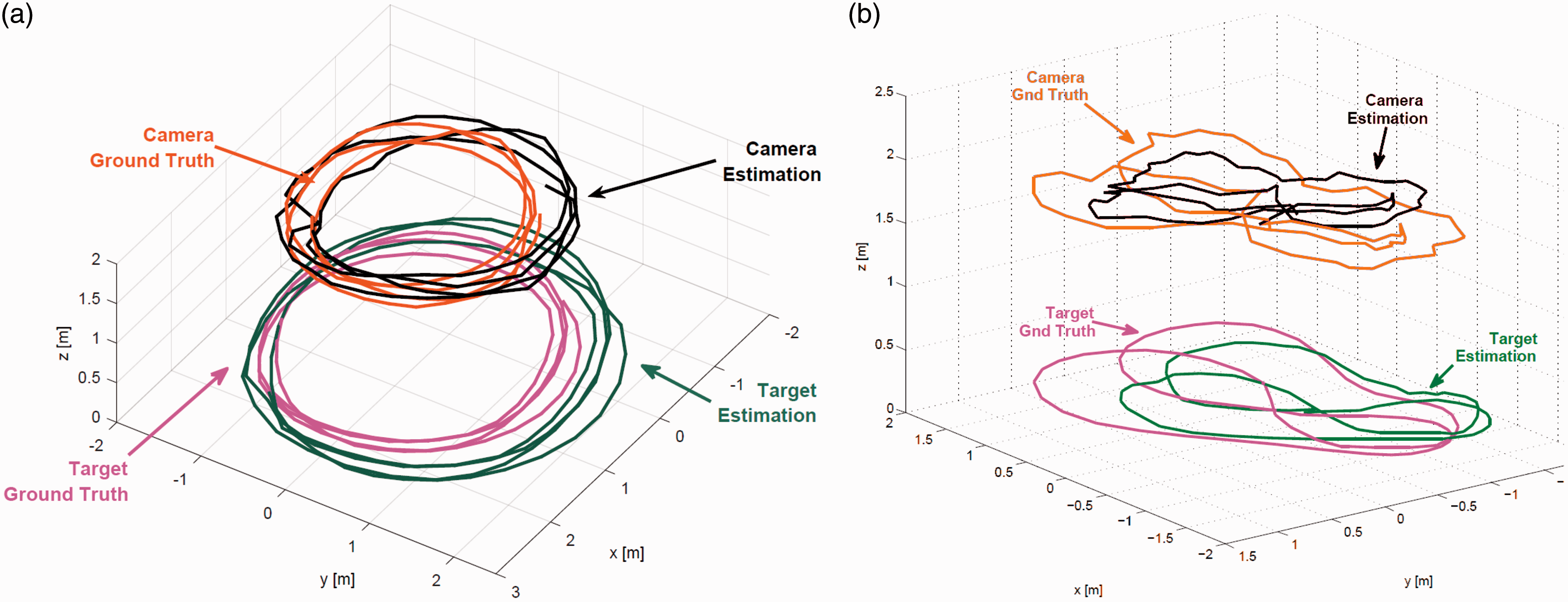
Estimated vs. ground truth 3D trajectories with real-imagery datasets for LBA approach in (a) ANPL1 dataset (b) ANPL2 dataset. BA approach produces similar results in terms of estimation errors, as shown in Table 2.

Figure 11.

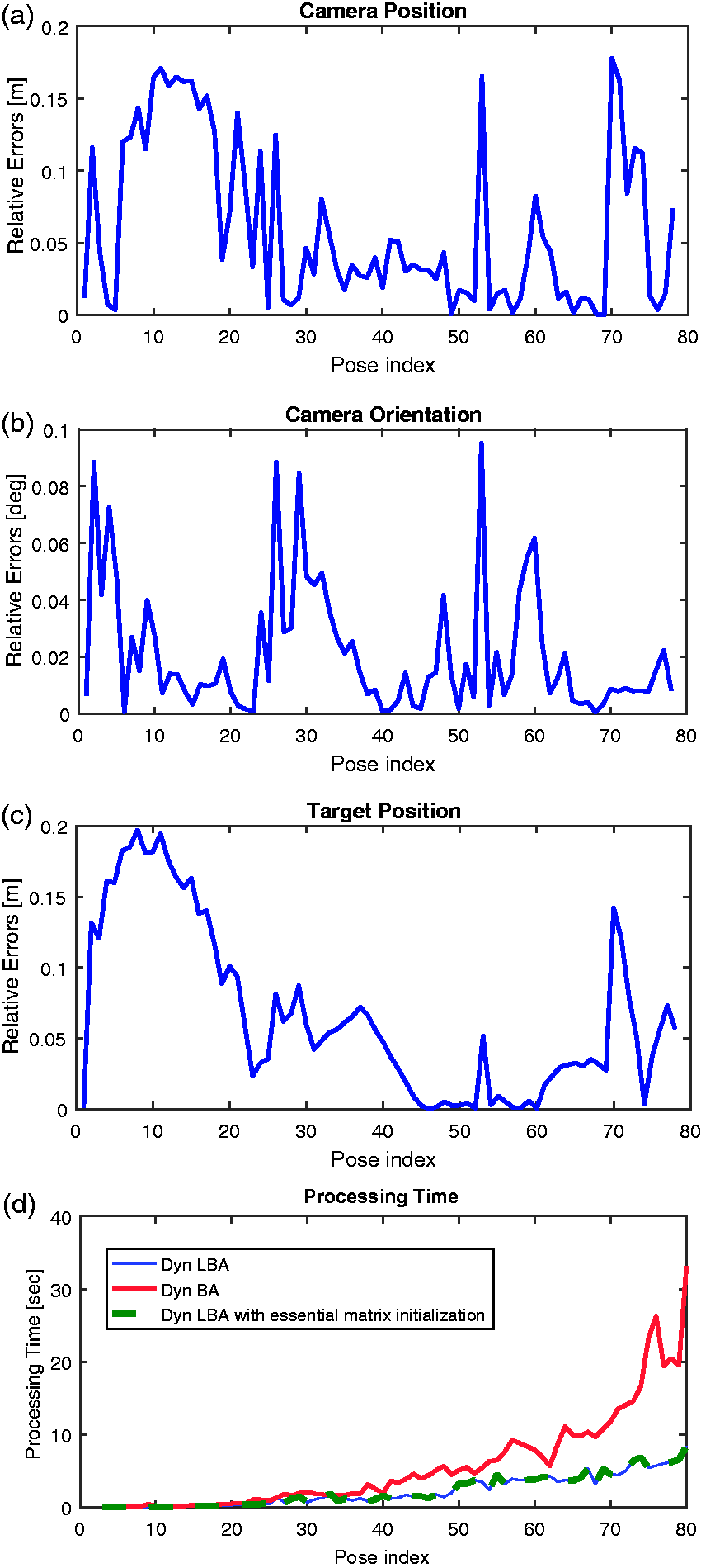
Incremental relative errors for the (a) camera position, (b) camera orientation, (c) target position, in ANPL1 dataset, (d) a comparison of the processing times per frame.

Tables 2 and 3 summarize the absolute values of the relative errors and the processing times for the two datasets. In both cases, the two methods show similar levels of accuracy: The average values for target and camera positions are 7 and 6 cm, respectively, for ANPL1 dataset, and 14 and 8 cm for ANPL2 dataset. In contrast, LBA with dynamic target tracking shows consequently better computational performances. The mean processing time per step is reduced by 61% for ANPL1 and by 39% for ANPL2.

Table 2.

Relative estimation errors summary of LBA method with respect to BA method for the camera and target positions in ANPL1 and ANPL2 datasets.

	Target position error (m)		Camera position error (m)
Dataset	Mean	Max	Mean	Max
ANPL1	0.07	0.19	0.06	0.18
ANPL2	0.14	0.42	0.08	0.34

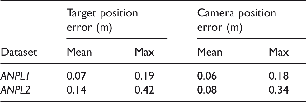
Note: The table entries are absolute values.

ANPL: Autonomous Navigation and Perception Lab.

Table 3.

Summary of the processing times with LBA and BA methods for the ANPL1 dataset.

		Processing time (s)
Dataset	Method	Mean	Total
ANPL1	BA	5.6	447.8
	LBA	2.2	177.1
ANPL2	BA	3.1	222.9
	LBA	1.9	139.4

LBA: light bundle adjustment; BA: bundle adjustment; ANPL: Autonomous Navigation and Perception Lab.

Conclusions and future work

We presented an efficient method for simultaneous ego-motion estimation and target tracking using the LBA framework. By algebraically eliminating the observed landmarks from the optimization, we allow the target to become the only reconstructed 3D point in the process. This reduces significantly the number of variables compared to full BA methods, and thus, allows for processing time improvements. We presented the mathematical process involved in the integration of the target tracking problem into the LBA framework, leading to a cost function that is formulated in terms of multi-view constraints, target motion model, and observations of the target. Computational efforts are further reduced by applying incremental inference over factor graphs representing the optimization problem, thus performing partial calculations at each optimization step.

We investigate the performance of the proposed approach and compare it to the corresponding BA formulation using synthetic and real-imagery datasets. While the two approaches exhibit similar accuracy levels, a significantly reduced running time was obtained for the proposed approach with both experimental methods. In particular, the presented method was up to seven times faster than full BA in the simulations and up to two and a half times faster in the real-imagery experiments. This difference, however, is expected to vary with the number of landmarks observed per frame. The created real-imagery datasets have been made available to the research community through the ANPL website. These datasets include recorded images with synchronized ground truth for both the camera and the target, and is seen as a contribution by itself.

As for future work, aerial experiments including scale estimation for both BA and LBA methods (potentially using fusion with additional sensors such as IMU) could further improve the realism of the scenario. Also, an experimental implementation of our method to the multi-target tracking problem seems a natural continuation. In this case, the method used for targets detection and data-association represents a real challenge.

Footnotes

Declaration of conflicting interests

The author(s) declared no potential conflicts of interest with respect to the research, authorship, and/or publication of this article.

Funding

The author(s) received no financial support for the research, authorship, and/or publication of this article.

References

T-D.

Vehicle perception: localization, mapping with detection, classification and tracking of moving objects. PhD Thesis, Institut National Polytechnique de Grenoble-INPG, France, 2009.

Wang

Thorpe

and Thrun

Online simultaneous localization and mapping with detection and tracking of moving objects: theory and results from a ground vehicle in crowded urban areas. In: IEEE international conference on robotics and automation (ICRA), Taipei, Taiwan, 2003, pp.842–849.

Eustice

Singh

Leonard

et al . Visually navigating the RMS titanic with SLAM information filters. In: Robotics: science and systems (RSS), Massachusetts, USA, 8-11 June, 2005.

Hover

Eustice

Kim

et al . Advanced perception, navigation and planning for autonomous in-water ship hull inspection. Int J Rob Res 2012; 31: 1445–1464.

Chekhlov

Gee

Calway

et al . Ninja on a plane: automatic discovery of physical planes for augmented reality using visual slam. In: Proceedings of the 2007 6th IEEE and ACM international symposium on mixed and augmented reality. Washington, DC, USA: IEEE Computer Society, 2007, pp.1–4.

6 Zhou

Been-Lirn

Duh H

, and Billinghurst

Trends in augmented reality tracking, interaction and display: a review of ten years of ISMAR. In: Proceedings of the 7th IEEE/ACM international symposium on mixed and augmented reality. IEEE Computer Society, Washington DC, USA, 2008, pp.193–202.

Lipton

Fujiyoshi

and

Patil

RS.

Moving target classification and tracking from real-time video. In: Proceedings fourth IEEE workshop on applications of computer vision. WACV’98. IEEE, USA, 1998.

Clendenin

and Freeman

RS.

Optical target tracking and designating system. US Patent 4,386,848, USA, 1983.

Wright

SE.

UAVs in community police work. AIAA Infotech@Aerospace 2005-6955, Arlington, Virginia, September 26 - 29, 2005.

10.

Neira

Davison

and Leonard

JJ.

Guest editorial special issue on visual slam.

IEEE Trans Rob 2008; 24: 929–931.

11.

Indelman

Roberts

and Dellaert

Incremental light bundle adjustment for structure from motion and robotics.

Rob Auton Syst 2015; 70: 63–82.

12.

Indelman

Bundle adjustment without iterative structure estimation and its application to navigation. In: IEEE/ION position location and navigation system (PLANS) conference, Myrtle Beach, SC, USA, 23-26 April, 2012.

13.

Indelman

Roberts

Beall

et al . Incremental light bundle adjustment. In: British machine vision conference (BMVC), Guildford, UK, 3-7 September 2012.

14.

Kaess

Johannsson

Roberts

et al . iSAM2: incremental smoothing and mapping using the Bayes tree. Int J Rob Res 2012; 31: 217–236.

15.

Dissanayake

MWMG

Newman

Durrant-Whyte

et al . A solution to the simultaneous localization and map building (SLAM) problem. IEEE Trans Rob Automat 2001; 17: 229–241.

16.

Smith

and Cheeseman

On the representation and estimation of spatial uncertainty. Int J Rob Res 1987; 5: 56–68.

17.

Konolige

Sparse sparse bundle adjustment. In:

British Machine Vision Conference (BMVC), Aberystwyth, Wales, UK, August 30 - September 2, 2010.

18.

Lourakis

MIA

and Argyros

AA.

SBA: a software package for generic sparse bundle adjustment. ACM Trans Math Softw 2009; 36: 1–30.

19.

Konolige

and Agrawal

FrameSLAM: from bundle adjustment to realtime visual mapping. IEEE Trans Rob 2008; 24: 1066–1077.

20.

Rodríguez

López de Teruel

and Ruiz

Reduced epipolar cost for accelerated incremental SFM. In: IEEE conference on computer vision and pattern recognition (CVPR), 2011, Providence, RI, pp.3097–3104.

21.

Steffen

, Frahm

J-M

and Förstner

Relative bundle adjustment based on trifocal constraints. In: ECCV workshop on reconstruction and modeling of large-scale 3D virtual environments, Greece, September 11, 2010.

22.

Eustice

Singh

and Leonard

JJ.

Exactly sparse delayed-state filters for view-based SLAM.

IEEE Trans Rob 2006; 22: 1100–1114.

23.

Ila

Porta

and Andrade-Cetto

Information-based compact pose SLAM.

IEEE Trans Rob 2010; 26: 78–93.

24.

Wang

C-C

and

Thorpe

Simultaneous localization and mapping with detection and tracking of moving objects. In: Proceedings 2002 IEEE international conference on robotics and automation (vol. 3). IEEE, Washington, DC, USA, 11-15 May, 2002, pp.2918–2924.

25.

Bar-Shalom

and Fortmann

TE.

Tracking and data association. New York: Academic Press, 1988.

26.

Huang

Zhou

Trawny

et al . A bank of maximum a posteriori (map) estimators for target tracking. IEEE Trans Rob 2015; 31: 85–103.

27.

Montesano

Minguez

and Montano

Modeling the static and the dynamic parts of the environment to improve sensor-based navigation. In: Proceedings of the 2005 IEEE international conference on robotics and automation. IEEE, Barcelona, Spain, 18-22 April, 2005, pp.4556–4562.

28.

Wang

C-C.

Simultaneous localization, mapping and moving object tracking. PhD Thesis, Robotics Institute, Carnegie Mellon University, Pittsburgh, PA, 2004.

29.

T-D

Burlet

and Aycard

Grid-based localization and local mapping with moving object detection and tracking.

Inform Fusion 2011; 12: 58–69.

30.

Ortega

JS.

Towards visual localization, mapping and moving objects tracking by a mobile robot: a geometric and probabilistic approach . PhD Thesis, Institut National Polytechnique de Toulouse-INPT, France, 2007.

31.

Hähnel

Schulz

and Burgard

Mobile robot mapping in populated environments.

Adv Rob 2003; 17: 579–597.

32.

Pancham

Tlale

and Bright

Literature review of SLAM and DATMO. 4th Robotics and Mechatronics Conference of South Africa (RobMech 2011), CSIR International Conference Centre, Pretoria, 23–25 November 2011

33.

Thrun

Burgard

and Fox

Probabilistic robotics. MIT Press, 2005.

34.

Hartley

and Zisserman

Multiple view geometry in computer vision. 2nd ed. Cambridge: Cambridge University Press, 2004.

35.

Bar-Shalom

Rong Li

and Kirubarajan

Estimation with applications to tracking and navigation: theory algorithms and software. New Jersey, USA: John Wiley & Sons, 2004.

36.

Kschischang

Frey

and Loeliger

H-A.

Factor graphs and the sum-product algorithm.

IEEE Trans Inform Theory 2001; 47: 498–519.

37.

Indelman

Gurfil

Rivlin

et al . Real-time vision-aided localization and navigation based on three-view geometry. IEEE Trans Aerosp Electron Syst 2012; 48: 2239–2259.

38.

Indelman

Navigation performance enhancement using online mosaicking . PhD Thesis, Technion, Israel Institute of Technology, Israel, 2011.

39.

Kaess

Ranganathan

and Dellaert

iSAM: incremental smoothing and mapping.

IEEE Trans Rob 2008; 24: 1365–1378.

40.

Fischler

and Bolles

Random sample consensus: a paradigm for model fitting with application to image analysis and automated cartography.

Commun ACM 1981; 24: 381–395.

Vision-based dynamic target trajectory and ego-motion estimation using incremental light bundle adjustment

Abstract

Keywords

Introduction

Problem formulation and notations

The BA problem

BA and target tracking

Factor graph representation

LBA and dynamic target tracking

LBA

LBA and dynamic target tracking

LBA and multi-target tracking

Incremental smoothing

Results

Experimental evaluation with synthetic datasets

Statistical simulation results

Large scenario

Experimental evaluation with real-imagery datasets

Conclusions and future work

Footnotes

Declaration of conflicting interests

Funding

References