Sage Journals: Discover world-class research

Abstract

This paper presents a framework for tracking a mobile ground target (MGT) using a fixed-wing unmanned aerial vehicle (UAV). Challenges from pure theories to practical applications, including varying illumination, computational limits and a lack of clarity are considered. The procedure consists of four steps, namely: target detection, target localization, states estimation and UAV guidance. Firstly, the MGT in the wild is separated from the background using a Laplacian operator-based method. Next, the MGT is located by performing coordinate transformations with the assumption that the altitude of the ground is invariant and known. Afterwards, a Kalman filter is used to estimate the location and velocity of the MGT. Finally, a modified guidance law is developed to guide the UAV to circle and track the MGT. The performance of our framework is validated by simulations and a number of actual flight tests. The results indicate that the framework is effective and of low computational complexity, and in particular our modified guidance law can reduce the error of the tracking distance by about 75% in specified situations. With the proposed framework, such challenges caused by the actual system can be tackled effectively, and the fixed-wing UAV can track the MGT stably.

Keywords

Fixed-wing UAV MGT Tracking Target Detection Target Localization

1. Introduction

Unmanned aerial vehicles (UAVs) are increasingly being used to replace manned aircraft for dull, dirty and dangerous (3D) missions [1]. The autonomous tracking of mobile ground targets (MGTs) reflects the particular advantages for UAVs in easing the burden on human operators, decreasing costs and allowing the increased manoeuvrability of the aircraft [2]. Tracking MGTs with UAVs is the foundation of their performance of important tasks like surveillance, reconnaissance and intelligence missions [3]. Although it has attracted a lot of research interest in recently years, most studies are either concerned with only one aspect [4 –7] of the tracking problem or else in pure theoretical terms [2, 8 –10]. Researchers still have a lot of work to do before UAVs can fully autonomously track MGTs. In this paper, we focus on the entire process of tracking a MGT using a fixed-wing UAV to address the challenges flowing from theory to practical applications.

There are two types of MGT tracking methods: one is cooperative and the other is non-cooperative. Under the cooperative method, such as in a convoy, the MGT is required to transmit its location to the UAV in real-time, whereas in the case of non-cooperative tracking (which is prevalent in the use of UAVs) the UAV is required to detect and localize the MGT in real-time. It is worth pointing out that the non-cooperative tracking of a MGT with a fixed-wing UAV is extremely challenging in an outdoor environment because of uncertainties as regards varying lighting conditions, motion and lack of clarity. Another challenge is the requirement of real-time operation with limited processing capacity provided by the onboard computer. The frame-rate of the onboard camera must be high enough and all the tasks must be completed as quickly as possible. Even in the worst case, the processing time must not exceed 33 ms [7, 11], which is considered to denote the real-time performance of a UAV. In this paper, we focus on the non-cooperative case in order to address the challenges stemming from theory to the practical application of MGT tracking using a fixed-wing UAV, including varying lighting conditions, limits in computational capability and lack of clarity caused by the actual system.

Different strategies have been proposed in the literature on MGT detection. Vision techniques and algorithms suitable for UAVs vary in complexity, ranging from simple colour segmentation to statistical pattern recognition. The relevant published works and proposed machine vision architectures indicate the use of both “onboard” [7, 12, 13] and “on-the-ground” [14, 15] processing setups. In [7], Kontitsis presents a template matching-based “onboard” target detection algorithm concerned with the limit in computational power, while the algorithm is proposed for a helicopter and evaluated in a traffic monitoring application. In such applications, the target in the image is larger and the relative velocity of the platform is much slower than that of a fixed-wing UAV.

Target localization is another essential process. Previously published studies mainly focus on unmanned ground vehicles [16] or hovering air vehicles, like blimps [17] and quadrotors [3, 18]. Meir Pachter et al. introduced a method in [19] for determining the location of a stationary ground target by using multiple micro air vehicles on the assumption that the object's altitude is known in advance. In [20], Barber et al. present a method to determine the GPS location of a stationary ground target using images from a fixed-wing miniature air vehicle. It is assumed that the target is identified from the video stream. For a stationary target, the UAV can easily circle around the target and collect enough information, while for a MGT both the circling and the collecting become more complicated. An autonomous tracking system also requires the UAV to adjust its path autonomously to collect additional information that is used to further enhance the estimate. In [10], a ground target tracking algorithm is proposed by Senqiang et al. On the assumption that the target location is known, their algorithm can be divided into two parts: a vector field-based guidance law, and a bang-bang controller. The guidance law produces a possible desired yaw of the UAV and the controller ensures that the UAV tracks the desired yaw. Simulation results demonstrate its effectiveness for a stationary ground target, while for a MGT there exists a large tracking error between the actual and desired distances. Extra modification is essential before the algorithm can be applied to track a MGT.

As reviewed above, most studies are either concerned with only one aspect of the tracking problem or else in pure theoretical terms. In this paper, we focus on the entire process of tracking a MGT with a fixed-wing UAV. A framework is developed considering the challenges of pure theory as well as of practical application. The procedure consists of four steps, i.e., target detection, target localization, states estimation and UAV guidance.

In most actual systems, the distance between a fixed-wing UAV and a MGT is greater than that of a helicopter or a traffic monitoring system, and a greater distance makes the target smaller and creates lack of clarity in the image. In such situations, neither traditional shape-based methods nor template-matching ones would work effectively. In our study, the MGT in the wild is not camouflaged and its reflections are different from the surroundings, which means that the greyscale value of the MGT is different from the natural surroundings. Due to the difference, we propose a Laplacian operator-based approach to detect the MGT. The Laplacian operator is based on the greyscale difference between the GMT and the background, and the greyscale difference is more robust to varying illumination than the greyscale value. After the Laplacian operator process, the influence of varying illumination can be reduced by using an adaptive threshold. Based on such an approach, the problem of occasional error identification can be tackled with a user-selection module, which makes the framework a supervised system. Next, the MGT can be located by performing a series of coordinate transformations. During this process, the distance sensor is absent from the onboard equipment, to which end the altitude of the ground is assumed to be invariant and known. Afterwards, a Kalman filter is used to estimate the position and the velocity of the MGT for noise suppression. Finally, a modified guidance law is developed to guide the UAV to track the MGT. In our guidance law, the desired yaw of the UAV is determined not only by the target position but also by the estimated target velocity and the current yaw of the UAV.

Notably, the computational complexity of the Laplacian operator-based detection approach in this work is much lower than that of the approach in [7], which is validated to work effectively in real-time on inexpensive and less powerful platforms. In addition, our modified guidance law can reduce the error of the tracking distance by about 75% in specified situations.

The main contribution of this paper is embodied in two ways. Firstly, regarding the practical applications, a useful framework for a fixed-wing UAV to track a MGT is proposed by considering the challenges caused by the actual system. In most existing studies, only aspects of the framework are considered and it is hard to apply them to the actual system directly. The proposed framework can locate a MGT with lower computational capacity, and consequentially can guide the UAV to track the MGT stably, which is certainly of great importance. Secondly, in order to decrease the gap between theory and practice, a number of real flight experiments are employed to verify the effectiveness of the proposed framework. The results convincingly show that our proposed framework can indeed tackle the challenges caused by practical applications, such as varying levels of light, computational limits and lack of clarity, which are seldom achieved in actual work.

The rest of the paper is organized as follows. In Section 2, we present the framework - specifically, from Section 2.1 to 2.4, we present the four steps of the procedure: target detection, target localization, states estimation and UAV guidance, respectively. In Section 3, we demonstrate the effectiveness of the entire framework via actual flight experiments. Finally, in Section 4, the paper is concluded with a few summaries and some future research directions.

2. Autonomous tracking framework

The flowchart of the proposed framework is shown in Figure 1. It includes four steps, namely target detection, target localization, states estimation and UAV guidance, which will be described in detail in the following subsections.

Figure 1.

Flowchart of the proposed framework for tracking a MGT using a fixed-wing UAV

2.1 Target detection

Figure 2 shows a frame obtained from a fixed-wing UAV. The target image is small and lacks clarity, while it is not camouflaged and its reflections are different from the surroundings. This is consistent with most practical applications. Therefore, in this work, the difference between the target and its surroundings is used as the key factor to isolate the MGT from an outdoor environment.

Figure 2.

An image obtained from a fixed-wing UAV, in which the distance from the UAV to the GMT is about 360 m

In our approach, first of all, part of the image is cut from the camera raw image and transformed into a greyscale image. Next, a Laplacian operator is performed on the greyscale image to sharpen the difference between the MGT and its surroundings. Afterwards, an adaptive threshold, a morphology operation and a fault rejection strategy are used to isolate the MGT from the input image. When occasional misidentification occurs, the user has to select the target at the ground control station. The block diagram of our approach is shown in Figure 3. The approach pipeline is shown in Figure 4.

Figure 3.

A block diagram of the target detection approach: (x_pu, y_pu) is the user's input and denotes the target's position in the pixel coordinate system

Figure 4.

Image processing pipeline

As shown in Figure 3, this part is responsible for receiving the user's input (x_pu, y_pu). The input is the target's position in the pixel coordinate system. It is essential at the beginning of the mission as well as when the system makes an error identification. Detailed methods and processes are presented as follows:

(1) Window selection

To reduce the computational load, the image processing is confined to a properly selected window. As the movement of the target and the UAV is continuous, the frame-rate of the camera is high enough and the target's position (x_p, y_p) in the current frame is close to (x_pl, y_pl), which is the target's position in the last frame. Therefore, a selected window around (x_pl, y_pl) can be cut from the current frame as shown in the second picture of Figure 4.

(2) Grey-scaling and Laplacian operator processing

The selected window is transformed into a greyscale image and the result is shown in the third picture of Figure 4.

In order to enhance sharp changes around the target and reduce smooth changes, the Laplacian operator as shown in Eq. (1) is introduced to process the greyscale image:

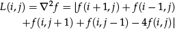
\begin{array}{l} L (i, j) = \nabla^{2} f = | f (i + 1, j) + f (i - 1, j) \\ + f (i, j + 1) + f (i, j - 1) - 4 f (i, j) | \end{array}

(1)

where f(i, j) is the greyscale value at point (i, j) in the pixel coordinate system and L(i, j) represents the output from the Laplacian operator.

Next, pixels around the target are enhanced and natural surroundings are reduced. The fourth picture of Figure 4 shows the output of the Laplacian operator.

(3) Adaptive thresholding

In general, the threshold value is highly sensitive to external influences, such as illumination. It is not feasible to determine a constant threshold value in actual outdoor tests. In this work, an adaptive threshold is introduced to address the influence of illumination. As shown in the fourth picture of Figure 4, the pixels around the target are enhanced and other smooth changes are reduced, so the threshold can be updated according to the maximum value in the output of the Laplacian operator L(i, j). Eq. (2) shows the adaptive threshold in our algorithm:

\begin{array}{l} T_{t h} = μ_{t h} \max (L (i, j)) \end{array}

(2)

where T_th denotes the adaptive threshold value and μ _th is an empirical coefficient. The result is shown in the fifth picture of Figure 4.

(4) Morphology operation and blob analysis

Morphology operation: After the threshold, low-level interference may remain in the binary image. Therefore, we perform a morphological opening on the binary image to remove this. The result is shown in the sixth picture of Figure 4.

Blob analysis: Connected components are labelled with a perimeter and size information.

(5) Fault rejection

It is possible that more than one target candidate remains in the selected window. In our work, a Ford Transit is used as the ground target, which is larger than most forms of interference, such as cars. Therefore, the largest element is isolated from all the target candidates as the MGT.

The proportion of the target pixels in the entire image is very low, as shown in Figure 2. Therefore, the target's position in the pixel coordinate system can be approximately determined by the centre of the largest target candidate. Small distortion is tolerable in the practice.

The performance of the target detection approach is tested in a series of frames obtained from an onboard camera. Some results are presented in Figure 5. However, error identifications are unavoidable for the blurry target image and the outdoor environment. When it occurs, the supervisor has to select the target through the user-selection component.

Figure 5.

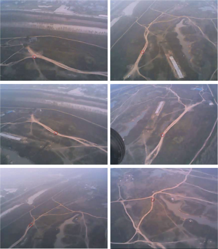
Test results of a series of frames from an onboard camera

By the proposed algorithm, the challenge of varying illumination from different angles of the UAV to the MGT can be effectively tackled. For our tracking system, the main computational load concerns image processing. Considering an identical selected image, the computational complexity involved in implementing the Laplacian operator is significantly less than that of a template matching method. In [7], the target is identified from the frame by performing an adaptive template-matching in a selected window, and the approach is validated to effectively work in real-time on inexpensive and less powerful platforms. Therefore, our approach works more efficiently in tackling the problem within computational ability limits. By the approach, the MGT in the wild can be detected (although it does not work in multi-target cases or in urban areas).

2.2 Target localization

In this section, we briefly describe our method for locating the MGT in the navigation coordinate system. In order to achieve this objective, related known and unknown information is listed as follows:

The target's pixel coordinates (x_p, x_p) are known from Section 2.1 .

The view angles C_x and C_y of the onboard camera are known in advance, which denote the viewing angles in axes X_p and Y_p respectively.

The orientation of the camera in the UAV body coordinate system can be described with direction and pitching angles, namely θ and φ, which can be measured with a pan-tilt unit (PTU).

The orientation of the UAV in the NED coordinate system can be described with yaw (or heading), pitch and roll angles, namely φ, η and β, which can be measured with an onboard IMU.

No distance sensor is included within the scope of the onboard equipment, while the altitude of the ground is known and the altitude of the UAV can be measured with a GPS module. Accordingly, the height of the UAV H_uav above the ground is known.

To explain our method clearly, the graphical interpretations of the reference frames are illustrated in Figure 6. The detailed description and definition of each of these coordinate systems are given in the following.

Figure 6.

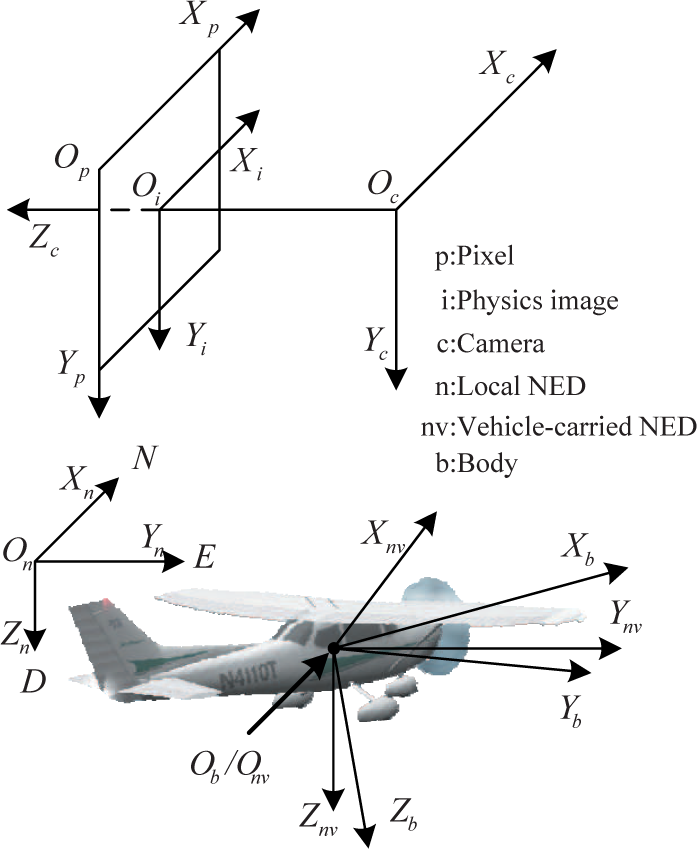
Reference frames: pixel, physics image, camera, local NED, vehicle-carried NED and UAV body coordinate systems

The pixel coordinate system O_pX_pY_p is centred in the upper left corner of the image and uses one pixel as a base unit. The X-axis X_p and Y-axis Y_p are, respectively, parallel to the rows and columns of the image.

The physics image coordinate system O_iX_iY_i is similar to the pixel coordinate system. Its origin O_i is the intersection of the optical axis and the image plane. The X-axis X_i and Y-axis Y_i are, respectively, parallel to X_p and Y_p.

The camera coordinate system O_cX_cY_cZ_c is defined on the camera. Its origin O_c is at the centre of projection of the camera. The X-axis X_c and the Y-axis Y_c are, respectively, parallel to X_p and Y_p. The Z-axis is taken as the optical axis of the camera (with points in front of the camera in the direction towards positive z).

The local NED coordinate system O_nX_nY_nZ_n is also known as a ground coordinate system. It is a coordinate frame fixed to the Earth's surface. Its origin and axes are defined as follows: the origin O_n is fixed to a point on the Earth's surface; the X-axis X_n points towards the geodetic north; the Y-axis Y_n points towards the geodetic east; and the Z-axis Z_n points downwards along the ellipsoid normal.

The vehicle-carried NED system O_nvX_nvY_nvZ_nv is associated with the UAV. It is defined as the navigation coordinate system. Its origin and axes are defined as follows: the origin O_nv is located at the centre of gravity of the UAV; the X-axis X_nv points towards the geodetic north; the Y-axis Y_nv points towards the geodetic east; and the Z-axis Z_nv points downwards along the ellipsoid normal.

The body coordinate system O_bX_bY_bZ_b is carried on the vehicle and is directly defined on the body of the UAV. Its origin and axes are defined as follows: the origin O_b is located at the centre of gravity of the UAV; the X-axis X_b points forwards, lying on the symmetric plane of the UAV; the Y-axis Y_b points to the right side of the UAV; and the Z-axis Z_b points downwards to comply with the right-hand rule.

We assume that O_c coincides with O_b and O_nv. Next, the transformation relationships among O_cX_cY_cZ_c, O_bX_bY_bZ_b and O_nvX_nvY_nvZ_nv are described by rotations alone. Another simplifying assumption is that the principle point is in the centre of the image. Following this, the coordinates' transformations among the coordinate systems are presented in Eq. (3)–(6). The transform relation between the pixel coordinate system and the vehicle-carried NED coordinate system is presented in Eq. (7):

\begin{array}{l} {[x_{i} ​ ​ y_{i} ​ ​ 1]}^{T} = K_{p}^{i} {[x_{p} ​ ​ y_{p} ​ ​ 1]}^{T} \end{array}

(3)

\begin{array}{l} {[x_{c} ​ ​ y_{c} ​ ​ z_{c}]}^{T} = z_{c} K_{i}^{c} {[x_{i} ​ ​ y_{i} ​ ​ 1]}^{T} \end{array}

(4)

\begin{array}{l} {[x_{b} ​ ​ y_{b} ​ ​ z_{b}]}^{T} = R_{c}^{b} {[x_{c} ​ ​ y_{c} ​ ​ z_{c}]}^{T} \end{array}

(5)

\begin{array}{l} {[x_{n v} ​ ​ y_{n v} ​ ​ z_{n v}]}^{T} = R_{b}^{n v} {[x_{b} ​ ​ y_{b} ​ ​ z_{b}]}^{T} \end{array}

(6)

\begin{array}{l} {[x_{n v} ​ ​ y_{n v} ​ ​ z_{n v}]}^{T} = z_{c} R_{b}^{n v} R_{c}^{b} K_{i}^{c} K_{p}^{i} {[x_{p} ​ ​ y_{p} ​ ​ 1]}^{T} \end{array}

(7)

where K _i ^p is the calibration matrix, K _i ^p K _i ^c is the projection matrix, R ^b _c is the rotation matrix from the camera frame to the body frame, and R ^nv _b is the rotation matrix from the body frame to the vehicle-carried NED frame:

\begin{matrix} K_{i}^{c} K_{p}^{i} = (\begin{matrix} 1 ∕ f & 0 & 0 \\ 0 & 1 ∕ f & 0 \\ 0 & 0 & 1 \end{matrix}) (\begin{matrix} d x & 0 & - o_{1} d x \\ 0 & d y & - o_{2} d x \\ 0 & 0 & 1 \end{matrix}) \\ = (\begin{matrix} d x ∕ f & 0 & - o_{1} d x ∕ f \\ 0 & d y ∕ f & - o_{2} d x ∕ f \\ 0 & 0 & 1 \end{matrix}) \end{matrix}

(8)

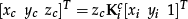
where (o₁, o₂) = (W_p/2, H_p/2) denotes the pixel coordinates for the point O_i, (W_p × H_p) represents the resolution of the camera and f/d_x, f/d_y specifies the pixel spacing in the X_p and Y_p directions. We can determine the values of d_x/f and d_y/f according to the known view angles C_x and C_y. The relation between them is shown in Eq. (9):

\begin{array}{l} d x ∕ f = 2 t a n (C_{x} ∕ 2) ∕ W_{p}, ​ ​ ​ ​ d x ∕ f = 2 t a n (C_{y} ∕ 2) ∕ H_{p} \end{array}

(9)

R ^b _c is determined by the orientation of the camera: θ, φ and R ^nv _b are determined by the orientation of the UAV: φ, η and β;

R_{c}^{b} = (\begin{matrix} C θ C φ ​ & - S θ ​ & C θ S φ \\ S θ C φ ​ & C θ ​ & S θ S φ ​ \\ - S φ ​ & 0 ​ & C φ ​ \end{matrix})

(10)

R_{b}^{n v} = (\begin{matrix} C η C ϕ ​ & S η S β C ϕ - C β S ϕ ​ & S η C β C ϕ - S β S ϕ \\ C η S ϕ ​ & S η S β S ϕ - C β C ϕ & S η C β S ϕ - S β C ϕ \\ - S η & C η S β & C η C β \end{matrix})

(11)

where C and S are abbreviations of sin() and cos(), respectively. As such, we can obtain [x_nv/z_c y_nv/z_c z_nv/z_c] ^T from Eq. (7). Eq. (7) is rewritten into in Eq. (12):

\begin{matrix} {[x_{n v} ∕ z_{c} ​ ​ y_{n v} ∕ z_{c} ​ ​ z_{n v} ∕ z_{c}]}^{T} = [x_{n v 0} ​ ​ y_{n v 0} ​ ​ z_{n v 0}]^{T} \\ = R_{b}^{n v} R_{c}^{b} K_{i}^{c} K_{p}^{i} {[x_{p} ​ ​ y_{p} ​ ​ 1]}^{T} \end{matrix}

(12)

where [x_nv0 y_nv0 z_nv0] can be calculated according to Eq. (12), and z_nv is equal to the height of the UAV H_uav. As such, we can get z_c = H_uav/z_nv0. Substituting z_c into Eq. (12), we can obtain the target's position in the vehicle-carried NED frame, as shown in Eq. (13):

\begin{matrix} {[x_{n v} ​ ​ y_{n v} ​ ​ z_{n v}]}^{T} = [x_{n v 0} ∕ z_{n v 0} ​ ​ y_{n v 0} ∕ z_{n v 0} ​ ​ H_{u a v}]^{T} \end{matrix}

(13)

In many missions, we need the target's position in other coordinate systems, such as the GPS position. In our work, the method in [21, 22] is used to transform [x_nv y_nv z_nv] into the GPS position.

2.3 Target states estimation

The MGT is located with measurements of the onboard PTU, camera, IMU and GPS module. There is noise in all of the measurements. However, in practice, the noise among the measurements is a Gaussian distribution with a mean 0. Therefore, a Kalman filtering approach is used to estimate the location and velocity of the MGT. The estimated velocity will be used to modify the guidance law presented in [10] in the next subsection.

2.4 UAV guidance law

This section aims to describe our method for guiding the UAV in tracking the GMT. This work is based on the method presented in [10]. With some modification, our method can be directly utilized to guide the fixed-wing UAV to track a MGT. In this work, we assume that the UAV is equipped with an inner-loop controller to track the desired yaw, that the target moves at a lower speed than the UAV, and that the UAV maintains a constant altitude and velocity. Accordingly, Dubin's model of the UAV can be formulated as Eq. (14):

\begin{array}{l} {\dot{x}}_{u} = v_{0} \cos ϕ \\ {\dot{y}}_{u} = v_{0} \sin ϕ \\ \dot{ϕ} = u \end{array}

(14)

where υ₀ is the constant velocity, x_u, y_u represent the 2D position of the UAV, φ is the yaw and u ∈ [−u_m, u_m] is the yaw rate with input constraints.

For a stationary target, as shown in Figure 7, the desired yaw of the UAV can be calculated according to the guidance law presented in [10], as shown in Eqs. (15)–(16), where φ_d ∈ [−π, π) is the desired yaw, r_d and r denote the desired and real horizontal distances from the UAV to the target, respectively, and ξ is the polar angle of the UAV.

Figure 7.

Ground target tracking with a fixed-wing UAV

ϕ_{d} = Φ_{s} + ξ

(15)

Φ_{s} = 2 \arctan (r ∕ r_{d})

(16)

In [10], the performance of the guidance law for a stationary target is illustrated by simulation results. The UAV orbits around the target in a set counter-clockwise direction, ignoring the current yaw of the UAV.

Consider that, when the UAV finds the target, the location and yaw of the UAV are (200m, 300m) and π/10. By the guidance law in [10], the tracking trajectory of the UAV is shown in Figure 8(a). It takes more time for the UAV to converge to the desired tracking trajectory. More seriously, the UAV may lose its tracking target because the distance between increases. In such a situation, a clockwise direction is more suitable for tracking, as shown in Figure 8(b). Therefore, to determine the circling direction of the UAV, the current orientation of the UAV should be taken into account. The modification is reflected in Eq. (19).

Figure 8.

Modification considering the current orientation of the fixed-wing UAV: (a) the original guidance law in [10], and (b) the modified guidance law in the framework

For a MGT, the performance of the guidance law in [10] is poor due to the neglect of the target motion. As such, another modification requires that the velocity of a MGT be taken into account. The modified guidance law is shown in Eqs. (17)–(19), where υ;_t is the speed of the mobile target and γ ∈ [−π, π) is the angle between the yaw and the line connecting the UAV with the target:

ϕ_{d} = Φ_{m} + ξ

(17)

Φ_{m} = 2 s i g n_{+} (γ) \arctan [(r ∕ r_{d})^{\max (v_{t},1)}]

(18)

s i g n_{+} (γ) = {\begin{array}{l} 1 & γ \geq 0 \\ - 1 & γ < 0 \end{array}

(19)

In the modified guidance law, (r/r_d)^{max(υ
_t
,1)} is used instead of r/r_d in Eq. (16). The purpose is to compensate the influence of the target velocity. The improvement of the modified method is:

If r < r_d, then r/r_d < 1 and (r/r_d)^max(υ_t,1) ≤ r/r_d, so Φ_m ≤ Φ_s < π/2. This means that when the actual tracking distance is smaller than the desired distance, the modified guidance law can guide the UAV to converge faster on the desired tracking trajectory than the original.

If r > r_d, then r/r_d > 1 and (r/r_d)^max(υ_t,1) ≥ r/r_d, so Φ_m ≥ Φ_s > π/2. This means that when the actual tracking distance is greater than the desired distance, the modified guidance law can guide the UAV to converge faster on the desired tracking trajectory than the original.

As a result, the modified guidance law can guide the UAV to converge faster on the desired tracking trajectory than the original. In order to illustrate the effectiveness of the modified guidance law, a simulation is conducted in which the bang-bang controller proposed in [10], as shown in Eq. (20), was used:

u = {\begin{array}{l} - u_{m} & ϕ_{d} - ϕ < 0 \\ u_{m} & ϕ_{d} - ϕ > 0 \end{array}

(20)

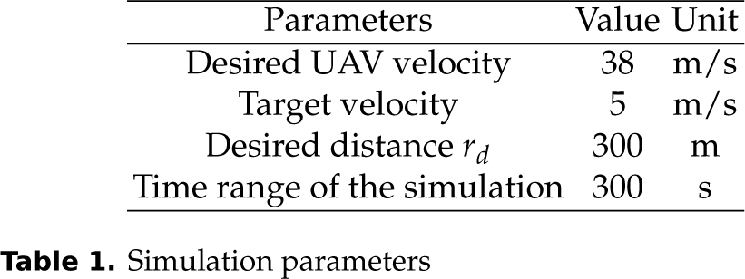
The main parameters in the simulation are listed in Table 1.

Table 1.

Simulation parameters

Parameters	Value	Unit
Desired UAV velocity	38	m/s
Target velocity	5	m/s
Desired distance r_d	300	m
Time range of the simulation	300	s

The simulation results are shown in Figure 9. Figure 9(a) shows that both the modified and original guidance laws can guide the UAV to circle and track the mobile target. Figure 9(b) shows the distance error of the two methods vary sharply. The distance error of the modified method is smaller than the original by 25%.

Figure 9.

Simulation results of the UAV guidance law: (a) tracking trajectory of the UAV, and (b) distance between the UAV and the target

3. Flight experiment

The framework was presented in Section 2, supported by some analyses and simulation results listed to illustrate the effectiveness of each part. In this section, a number of actual flight experiments are performed to demonstrate the effectiveness of the entire framework.

3.1 System setup

A flight experiment system for the framework was developed. The block diagram of the experimental system is shown in Figure 10. In the experimental system, The UAV as shown in Figure 11 is used as the platform. Its main characteristics are listed in Table 2. The platform is equipped with an IFLY-F1 controller that deals with the inner control loop of the UAV. Thus, the IFLY-F1 controls the vehicle dynamics, setting the control surface's deflections and the engine power required to follow the references provided by the proposed framework.

Table 2.

Specifications of the experimental UAV prototype

Parameters	Value	Unit
Wingspan	2.9	m
Maximum weight	15	Kg
Payload	5	Kg
Maximum speed	40	m/s
Autonomy	1	h

Figure 10.

Block diagram of the flight experiment system

Figure 11.

Fixed-wing UAV platform with onboard equipment including a PTU, camera and GPS module

In addition to the autopilot, the UAV is equipped with an onboard computer, a FLIR PTU and an onboard camera. The PTU is used to aim the camera at the MGT. The onboard camera provides real-time digital images (640*480, 30 fps) to the onboard computer through USB2.0 and transmits real-time videos to the ground control station through a 5.8 GHz transmitter. The frequency of the data link between the UAV and the ground control station is 902–928 MHz. The main computational load of the framework is the target detection process. Analysis results in Section 2.1 show that the computational complexity is much lower than that in [7], where the approach is validated to effectively work in real-time on inexpensive and less powerful platforms. Thus, in the flight experiment system, a ThinkPad X220 is used as the onboard computer to save time for hardware development. The onboard program was developed in the C++ programming language based on the OpenCV library. Meanwhile, a Ford Transit was used as the MGT, whose actual trajectory during the mission was measured with a GPS module with a precision of CEP 2.0 m.

3.2 Test of the proposed framework

In the flight experiment, the altitude of the ground was about 37 m, which was assumed to be invariant. The target moves at a speed of 2–10 m/s from the initial location (112.9353, 28.2953). The frequency of the target recognition is 30 fps. The main experiment parameters are listed in Table 3. The flight experiment results are shown in Figures 12 –16.

Table 3.

Flight experiment parameters

Parameters	Value	Unit
Desired UAV velocity	38	m/s
Target velocity	2–10	m/s
Desired distance r_d	300	m
Height of the UAV	200	m
Time range of the flight	240	s

Figure 12.

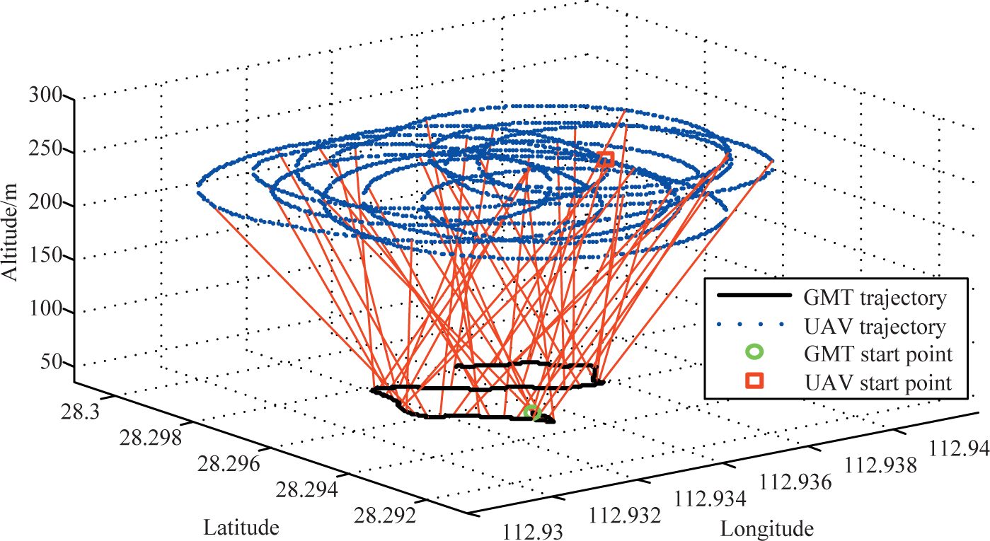
Tracking trajectory of the UAV in the duration of the flight experiment

Figure 13.

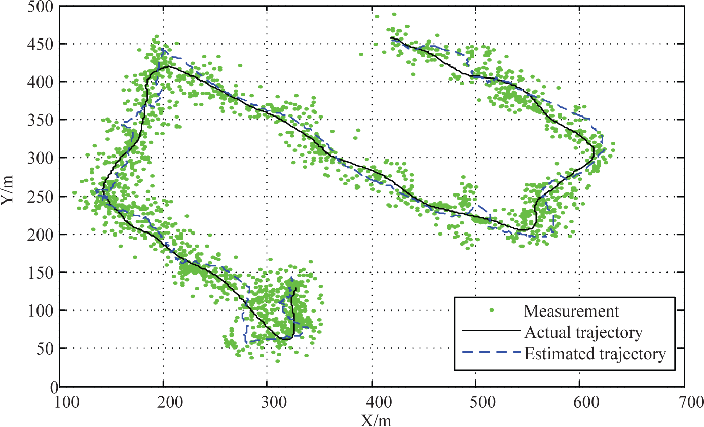
Target trajectories during the flight experiment including the measurement, the actual and estimated trajectories

Figure 14.

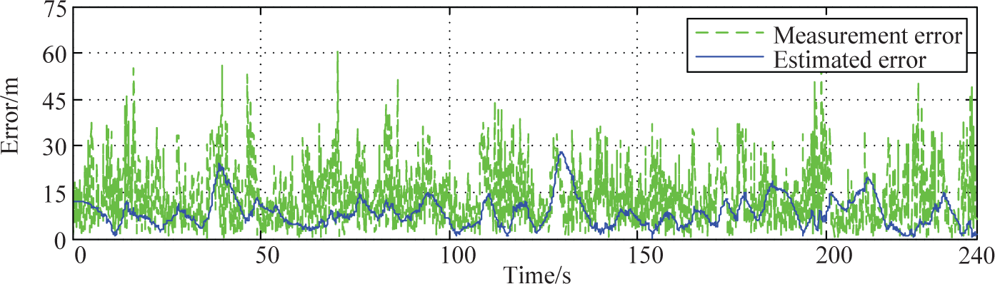
Location errors during the flight experiment including the measurement and the estimated

Figure 15.

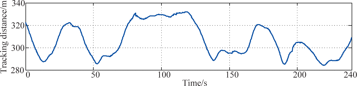
Tracking distance from the UAV to the MGT with a desired value of 300 m

Figure 16.

Target velocities including the actual and the estimated velocities during the flight experiment

The trajectories of the UAV and the MGT during the flight experiment shown in Figure 12 are measured with an onboard GPS module and a vehicle-mounted GPS module, respectively. It shows that the UAV can stably circle and track the MGT.

The trajectories of the MGT, including the measurements, the estimated trajectory and the actual trajectory, are shown in Figure 13. In order to make a quantitative analysis of the experiment results, the longitude and latitude data are transformed into metre-scaled data with the point (112.932, 28.294) as the origin, X pointing to the east and Y pointing to the north. In Figure 13, the “actual trajectory” is measured with a vehicle-mounted GPS module. The measurement points are the target localization results. It is shown that there are large errors in the location measurement of the MGT. The maximum value of the measurement errors is about 60 metres. Four main possible reasons are listed as follows:

Occasional misidentification: the misidentification may bring about much greater error than other factors.

Lack of synchronization or delays of the data obtained from sensors such as the onboard PTU, IMU, camera and GPS module.

The onboard camera we use is not accurately calibrated and the assumptions that we made in Section 2.2 are not always in accord with the actual instance.

There is no correction or orthorectification in the target detection part.

Figure 13 shows that the estimated trajectory of the MGT is much more reliable than the measurements. The location errors of both the measurements and the estimated results are given in Figure 14. It shows that the number of frames is 10 when the location error is greater than 45 m. The most possible reason for such an error is a misidentification. In this case, the supervisor at the ground control station has to correct the misidentification through the user-selection component. In the four-minute flight test, the user-selection component works 10 times (from 4 × 60 × 30 f ps) except for the first frame, at the beginning. In addition, the average error of the estimated locations of the MGT is about 8 m. The accuracy is sufficient for the tracking problem.

As shown in Figure 15, the actual tracking distance from the MGT to the UAV deviates more from the desired value than the simulation results, with the possible reasons are listed as follows:

Error of the localization: the maximum value of the error is 28 m and the average is 8 m.

Influence of wind, which is not considered in this work.

Poor tracking capability of the inner loop controller of the UAV, which needs promotion in future work.

The velocity curves of the MGT are shown in Figure 16. The “actual speed” is obtained from the vehicle-mounted GPS module and the “estimated speed” is obtained from the Kalman filter. It shows that the estimated speed matches the actual value well. In addition, the effectiveness of the framework is illustrated with the flight experiments in the wild, and all the elements, including target detection, target localization, states estimation and UAV guidance, function well.

4. Conclusion and future work

In this paper, we proposed a framework for a single fixed-wing UAV to track a MGT. The proposed framework can locate a small moving vehicle by using a single camera with lower computational complexity, and consequently can guide the UAV to track the moving target stably. The effectiveness of the framework is validated by simulations and a number of flight experiments. The results show convincingly that our proposed framework can indeed tackle the challenges caused by practical applications, such as varying illumination, computational limits and lack of clarity. In particular, the modified guidance law can reduce the error of the tracking distance by about 75% under specified situations. This work will contribute to the autonomous applications of UAVs from pure theory to practice.

Throughout this paper, we have focused on tracking a GMT in the wild using a single fixed-wing UAV. The target detection approach and the entire proposed framework were not developed for tracking multiple targets. Therefore, in future research, we will concentrate on the problem with multiple UAVs and multiple targets, which is much more complex in applications. Meanwhile, the kinetics and inner loop control of fixed-wing UAVs will be considered to improve their performance. Moreover, a more complex environment will be considered and the influence of the wind will be taken into account in future work.

Footnotes

5. Acknowledgements

This work was supported by the Research Project (No. JC-13–03–02) of the National University of Defence Technology. The authors would like to thank Lincheng Shen, Tianjiang Hu, Zhenqi Wang, Guosheng Ouyang and Zufeng Ye for their great help during the flight experiments.

References

Office of the Secretary of Defense (2007) Unmanned Systems Roadmap: 2007–2032.

Xiaowei

Huicheng

Xiaoguang

(2012) UAV Mobile Ground Target Pursuit Algorithm. J. intell. robot. syst. 68(3–4):359–371.

Gomez-Balderas

J E

Flores

Carrillo

L R Garcìa

Lozano

(2013) Tracking a Ground Moving Target with a Quadrotor Using Switching Control. J. intell. robot. syst. 70(1–4):65–78.

Frew

E W

Lawrence

D A

, and Morris

(2008) Coordinated Standoff Tracking of Moving Targets Using Lyapunov Guidance Vector Fields. Journal of guidance, control, and dynamics. 31(2):290–306.

Beard

R W

McLain

T W

Nelson

D B

Kingston

Johanson

(2006) Decentralized Cooperative Aerial Surveillance Using Fixed-wing Miniature UAVs. Proc.IEEE. 94(7):1306–1324.

Prévost

Thériault

Desbiens

Poulin

Gagnon

(2009) Receding Horizon Model-based Predictive Control for Dynamic Target Tracking. In: AIAA Guidance, Navigation, and Control Conference. August; Chicago.pp.1–9.

Kontitsis

Valavanis

(2010) A Cost Effective Tracking System for Small Unmanned Aerial Systems. J. intell. robot. syst. 57(1–4):171–191.

Zhu

Danwei

Low

C B

(2013) Ground Target Tracking Using UAV with Input Constraints. J. intell. robot. syst. 69(1–4):417–429.

Hyondong

Seungkeun

Hyo-Sang

Brian

A W

Antonios

Camille

A R

(2013) Rendezvous and Standoff Rarget Tracking Guidance Using Differential Geometry. J. intell. robot. syst. 69(1–4):389–405.

10.

Zhu

Danwei

(2012) Adversarial Ground Target Tracking Using UAVs with Input Constraints. J. intell. robot. syst. 65(1–4):521–532.

11.

Kim

H J

Mingu

Hyon

Chulwoo

Seungho

Daewon

Hyunjin

Gyeongtaek

Jongho

Youdan

(2013) Fully Autonomous Vision-based Net-recovery Landing System for a Fixed-wing UAV. IEEE transactions on mechatronics. 18(4):1320–1333.

12.

Mejias

Saripalli

Sukhatme

Cervera

(2005) Detection and Tracking of External Features in an Urban Environment Using an Autonomous Helicopter. In IEEE International Conference on Robotics and Automation(ICRA). Barcelona Spain.

13.

Anderson

J D

Lee

D J

Edwards

Archibald

Greco

C R

(2007) Real-time Feature Tracking on an Embedded Vision Sensor for Small Vision-guided Unmanned Vehicles. In: Proceedings of IEEE International Symposium on Computational Intelligence in Robotics and Automation. Jacksonville, FL, USA.

14.

Vidal

Sastry

(2002) Vision Based Detection of Autonomous Vehicles for Pursuit Evasion Games. In: the 15th Triennial World Congress. Barcelona, Spain.

15.

Hrabar

Sukhatme

G S

(2003) Omnidirectional Vision for an Autonomous Helicopter. In: Proceedings of IEEE International Conference on Robotics and Automation (ICRA). Taipei, Taiwan, pp.3602–3609.

16.

Saeedi

Lowe

D G

Lawrence

P D

(2003) 3D Localization and Tracking in Unknown Environments. In: Proceedings of the IEEE Conference on Robotics and Automation (ICRA). Taibei, Taiwan, pp.1297–1303.

17.

Chaimowicz

Grocholsky

Keller

J F

Kumar

Taylor

C J

(2004) Experiments in Multirobot Air-ground Coordination. In: the Proceedings of IEEE International Conference on Robotics and Automation(ICRA). New Orleans, LA, pp.4053–4058.

18.

Oliveira

Encarnação

(2013) Ground Target Tracking Control System for Unmanned Aerial Vehicles. J. intell. robot. syst. 69(1–4):373–387

19.

Pachter

Ceccarelli

Chandler

P R

(2008) Vision-based Target Geolocation Using Micro Air Vehicles. Journal of guidance, control, and dynamics. 31(3):597–615.

20.

Barber

D B

Redding

J D