DANCER: The routing algorithm in delay tolerant networks based on dynamic and polymorphic combination of dimensions and energy consideration

Abstract

Be differ from traditional networks, the nodes in delay tolerant networks are connected intermittently and they are mobile continuously, which result in high transmission delay and low delivery ratio. In addition, the energy of the mobile node is finite. Due to these constraints, efficient routing in delay tolerant networks is a tough task. In order to achieve higher routing efficiency in delay tolerant networks, we propose DANCER in this article, which utilizes a binary topology for more accurate and energy-efficient routing in delay tolerant networks. First, inspired by the concept of dimension in general relativity; the distance is diverse in different dimensions. Each node builds its own topology and the nodes in each topology are ranked in the top s in multiple dimensions. The link weight, which reflects the packet delivery ability between the two nodes in the topology, is defined by the reciprocals of ranking values of the two nodes in multiple dimensions and the reciprocals of important coefficients of each dimension. Second, due to each node has limited energy, Nash equilibrium solution is utilized to simplify the topology to determine which links are useful for a specific packet relaying. After simplification, each node obtains the binary topology which consists of links where flag bits are respectively 1 or 0. Finally, based on the binary topology, each node could decide the suitable routing for every specific packet sending. The result of the simulation demonstrates that DANCER outperforms benchmark routing algorithms in the respect of average delay, packets hit rate, and routing cost.

Introduction

Delay tolerant networks (DTNs) are a special type of challenged networks which have been applied to pocket switch networks (PSNs), underwater acoustic sensor network (UASN), and vehicular ad hoc network (VANET).^1–5 Compared with traditional networks, DTNs have three obvious characteristics, which are intermittent connectivity, dynamic network topology, and constrained node energy, so routing in this scenario is a tricky issue. In recent years, several benchmark routing schemes of DTNs have been proposed, for instance, Epidemic,^6,7 Prophet, ⁸ SimBet,^9,10 Bubble Rap, ¹¹ CAR, ¹² HiBop, ¹³ and SMART. ¹⁴

Epidemic is a flooding-based routing scheme for maximizing the hit rate of the packets. What comes with this flooding mode is the huge routing cost. Probabilistic routing scheme utilizes the history encounters of nodes’ to measure the delivery ability. Although it could avoid the disadvantage in Epidemic, its limited local view in forwarder selection may miss the longer and better forwarding opportunities. SimBet and Bubble Rap are sociality routing protocols: SimBet exploits two social metrics which are node similarity and ego betweenness to determine the next suitable node to delivery to; Bubble Rap uses different ways (which utilizes two aspects of the social network: centrality and community) to decide the suitable routing. However, those social routing protocols do not consider other attributes of the node. HiBop and CAR use the node’s multiple attributes which also called contextual information to obtain the potential routing, but these two schemes are devise based on the assumption that each node of network cooperates to receive and send the packets (relaying includes receiving and sending). However, in reality, the energy of each node is limited.^6,15–17

For example, in Figure 1, node a sends a packet which destination ID is p to the encountered node. Although the packet queue of the encountered node is not full, the energy of this node is shortage. Eventually, the encountered node will not receive the packet.

Figure 1.

Example of the encountered node’s energy is shortage.

In Figure 2, the encountered node has enough energy but the packet queue is full, so the encountered node will not receive the packet.

Figure 2.

Example of the encountered node’s packet queue is full.

In Figure 3, the encountered node has enough energy and the packet queue is not full. But in this case, the encountered node will trade off the payoffs and energy consumption to decide whether to relay the packet.

Figure 3.

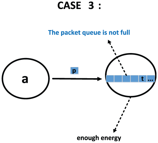
Example of the encountered node’s energy is enough and packet queue is not full.

When a node receives packets or sends packets, it will generate some energy consumption as well as get some payoffs (i.e. some energy supplement). For example, in Figure 4, node a sends packet to node b, and node a will generate some energy consumption and payoffs caused by sending the packet. Meanwhile, node b will generate some energy consumption and payoffs caused by receiving the packet.

Figure 4.

Example of the energy consumption and payoffs caused by sending or receiving packets.

Due to the selfishness of each node, they will trade off the energy consumption and payoffs to decide whether to relay the packet. In this article, we use Nash equilibrium ¹⁸ solution to address this issue.

The SMART ¹⁴ is an innovative routing algorithm, it is the first time that proposes the social map of each node, but it suffers from two problems: one problem is that it is based on the assumption that all nodes in social map cooperate to relay packets, but this is not realistic. For example, in Figures 1 and 5, node a sends packet to node b, but node b refuses to receive it. In Figures 2 and 5, node a sends packet to node b, and node b receives the packet but drops it. As a result of that, the hit rate of packets will be declined; the average delay and routing cost will be increased accordingly. Another problem is that the definition of the link weight in social map is based on the past encounter frequency of two nodes, but this is not accurate, because there are some invalid encounter frequencies (i.e. the contact duration is extremely short).

Figure 5.

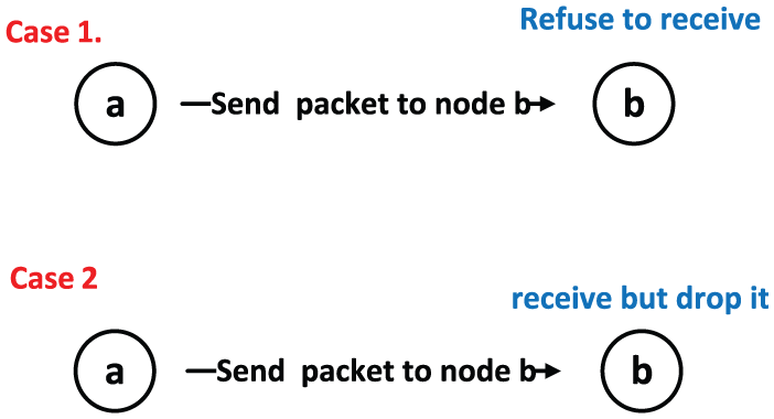
The results of case 1 and case 2.

To overcome these shortcomings, we propos DANCER, which exploits the binary topology constructed by each node to route in DTNs. The binary topology is constructed by the dynamic and polymorphic combination of dimensions and Nash equilibrium solution. Before talking about the link weight in binary topology, we assume that the two nodes associated with in the link are both ranked in the top s in g (g > the threshold value) dimensions; the link weight in binary topology is based on two factors: one is the reciprocal of the ranking values in g dimensions and another is the importance coefficient of each dimension. When each node obtains the link weights in its own binary topology, Nash equilibrium solution will be utilized to determine whether a link in binary topology is enabled in a specific data packet routing. In conclusion, this article makes the following contributions:

• First, we introduce a topology construction process based on the dynamic and polymorphic combination of dimensions.

• Second, using Nash equilibrium solution, we introduce the simplifying process to obtain the binary topology.

• Third, based on the binary topology, we propose a novel routing scheme with better performance.

The remainder of this article is organized as follows: In section “Related work,” we discuss some related works. In section “The DANCER routing scheme design,” we introduce the detailed design of DANCER. In section “Simulation and evaluation,” we describe the evaluation methodology. Finally, we give some conclusion about this article and raise further research issues.

Related work

In recent years, many researchers have proposed many well-designed routing strategies to enable asynchronous communication in intermittently connected ad hoc networks. Those classical routing strategies in disconnected DTNs include SimBet, ¹⁰ Epidemic,^6,7 Prophet, ⁸ CAR, ¹² and SMART. ¹⁴

SimBet routing scheme ¹⁰ utilizes two popular social metrics, ego betweenness and node similarity, to calculate the SimBetUtil value and select the next available node to relay to. This routing scheme is multicast based as it sends the packet to a selected number of neighboring nodes, thereby avoiding network flooding. However, different from DANCER, it just uses the social dimension of the node to decide the suitable routing.

Epidemic routing protocol^6,7,19 was inspired from the theory of Epidemic algorithms. When two nodes are close to each other, the summary vectors of the nodes are to be exchanged. After these exchanges, messages spread through the network as nodes meet and infect other nodes. Different from Epidemic routing, each node of DANCER uses the binary topology to guide the node’s routing instead of the flooding mode, so that DANCER will cost less energy.

Prophet^8,20 utilizes the past encounters and transitivity to calculate the delivery predictability. The relaying algorithm of Prophet is similar to the Epidemic algorithm except that messages are exchanged only if the receiving nodes have greater delivery predictability to the destination. For this reason, Prophet only has a limited routing view. Different from Prophet, DANCER uses multiple dimensions to decide the suitable routing which can obtain a more accurate routing scheme.

CAR ¹² utilizes contextual information to predict the probability of packet relay. The contextual information may include many attributes. The utility function has been applied by CAR to choose the suitable node with the highest probability of relaying a packet to its destination. In addition to the different ways of using the contextual information, DANCER further removes the assumption that each node cooperate to relay the packet.

SMAERT ¹⁴ is the pioneering social map–based routing schemes which exploit a distributed social map for lightweight routing in DTNs but it just uses one dimension to define the link weight. Be differ from the SMART, DANCER utilizes multiple dimensions to define a more accurate link weight.

The above routing schemes are all based on the assumption that nodes in network are cooperate to relay the packets. While in DANCER, we remove this assumption and use Nash equilibrium solution to determine whether a node is suitable for relaying the packets.

The DANCER routing scheme design

In this part, we first introduce the construction process of the topology. Then we utilize Nash equilibrium solution to simplify the topology to obtain the binary topology. After simplified, the binary topology will be consisted of links, where the flag bits are 1 or 0. Finally, we propose the routing strategy based on the binary topology.

The construction process of topology

Preface

DTNs are always applied to specific scenario (i.e. human-associated), such as the intelligent mobile devices that associated with humans, they inevitably demonstrate some of the social aspects associated with human-to-human communications, and it is also a fact that human social behaviors determine data communications. Actually, these are the attributes or the context information^12,13 of the mobile node. Inspired by the concept of dimensions in general relativity, ²¹ the distance between nodes is different in diverse dimensions. For the distance, it should be discussed in a specific dimension, because a long distance in one dimension may be a short distance in another dimension. For example, there are two ants, respectively, in two endpoints of the diagonal line of a paper; for the two ants, the distance is far while if we fold this piece of paper along the diagonal line, it will generate the third dimension (height), where it is close for the ants.

In another example, in Figure 6, for the family dimension and the geographic dimension, Jason would rather communicate with his distant families than with his closely neighbors. The distance on the family dimension is short, and the geographical dimension has little effect on the distance. In this article, we exploit multiple dimensions to represent these attributes of each node. These dimensions contain the following contents:

• The moving speed;

• The geographic location;

• The hobby (i.e. basketball, baseball);

• The dwell time at a location;

• The social hierarchy (i.e. super star, mayor);

• The age span (i.e. 3-year age difference, 10-year age difference);

• Whether they belong to the same family;

• The history encounters frequency;

• The communication radius;

• The common economic background.

Figure 6.

The different distances in two dimensions.

Figure 7.

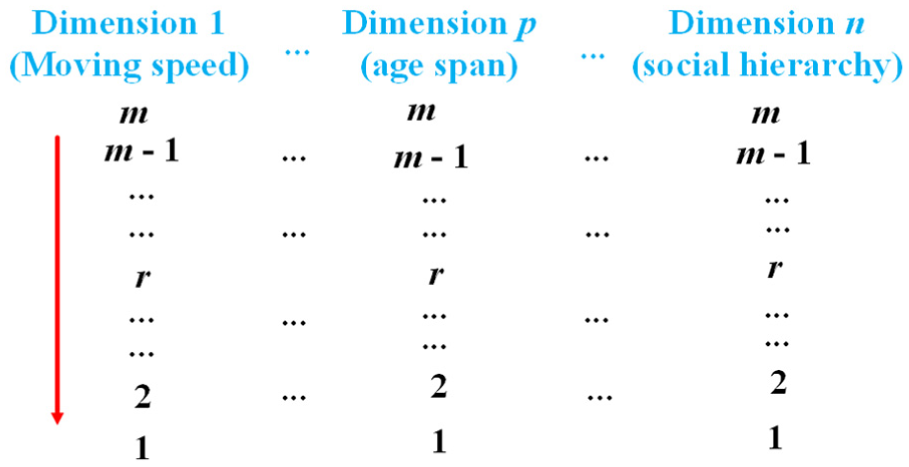
The rank division in each dimension.

In a word, we can define all dimensions can be imagined. Some dimensions are influenced to each other, such as the past encounter frequency is always related to the moving speed of the node and the two nodes’ dwell time at the encountering place. Some dimensions are independent to each other, like the social hierarchy and the moving speed. In different dimensions, the node’s ranking are diverse, what’s more, as time goes by, the node’ s ranking will be changed. In this article, importance coefficient will be used to represent the importance of a particular dimension to a node.

The attributes values classification

Definition 1

We divided each dimension D_i in the dimension set {D₁, D₂, D₃,…, D_i,…, D_n} into m (m ∈ [1, +∞)) ranks. As shown below, starting form rank 1, m is the maximum ranking value in ascending order.

After collected the attribute values of each node in each dimension, we classify these attribute values in each dimension separately. For example, as shown in Figure 8, the moving speed of node a is 100 m/min. Therefore, we classify it as the first rank in the moving speed dimension.

Figure 8.

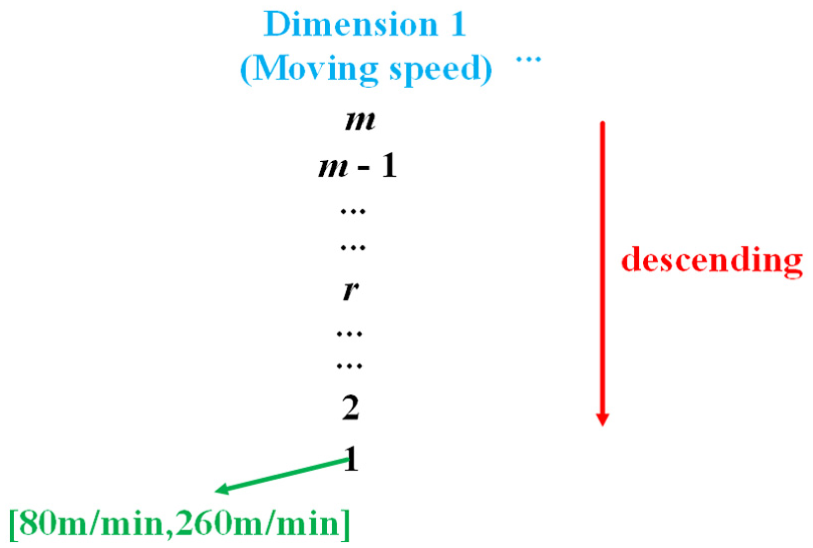
The example of attribute value classification.

For each dimension, we focus on these nodes which are ranked in top s(s <= m). As shown in Figure 9, the top s ranking scope is from rank r − s+1 to rank r.

Figure 9.

The top s rank scope.

Definition 2

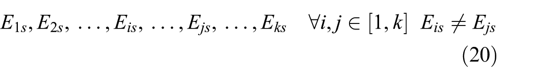
For each node, we use the n-dimensional vector HV to identify. Each value H in vector is an integer and these values represent the ranking value in each dimension

$$\mathrm{HV}=\left[\begin{array}{cccc}\begin{array}{cc}\begin{array}{cc}{H}_1\hfill & H_2\hfill \end{array}\hfill & \cdots \hfill \end{array}\hfill & H_p\hfill & \cdots \hfill & H_n\hfill \end{array}\right]$$

(1)

The importance coefficient vector

Definition 3

Assume there are k (k >= 1) nodes and n (n >= 1) dimensions. For a certain node a, the n-dimensional vector is shown as follows

$$H{V}_a=\left[\begin{array}{cccc}\begin{array}{cc}\begin{array}{cc}{H}_{a1}\hfill & H_{a2}\hfill \end{array}\hfill & \cdots \hfill \end{array}\hfill & H_{\mathrm{ap}}\hfill & \cdots \hfill & H_{\mathrm{an}}\hfill \end{array}\right]$$

(2)

The following equation is used to normalize the vector HV_a to obtain the normalized vector TV_a

$$T{V}_a=\left[\begin{array}{cccc}\begin{array}{cc}\begin{array}{cc}{T}_{a1}\hfill & T_{a2}\hfill \end{array}\hfill & \cdots \hfill \end{array}\hfill & T_{\mathrm{ap}}\hfill & \cdots \hfill & T_{\mathrm{an}}\hfill \end{array}\right]$$

(3)

$$T_{\mathrm{ap}}=\frac{H_{\mathrm{ap}}-H_p^{min}}{H_p^{max}-H_p^{min}}a\in [1,k]p\in [1,n]$$

After normalization, the vector TV_a is shown as follows

$$T{V}_a=\left[\begin{array}{cccc}\begin{array}{cc}\begin{array}{cc}\frac{H_{a1}-H_1^{min}}{H_1^{max}-H_1^{min}}\hfill & \frac{H_{a2}-H_2^{min}}{H_2^{max}-H_2^{min}}\hfill \end{array}\hfill & \cdots \hfill \end{array}\hfill & \frac{H_{\mathrm{ap}}-H_p^{min}}{H_p^{max}-H_p^{min}}\hfill & \cdots \hfill & \frac{H_{\mathrm{an}}-H_n^{min}}{H_n^{max}-H_n^{min}}\hfill \end{array}\right]$$

(4)

$H_p^{min}$ represents the minimum ranking value in dimension p(p ∈ [1, n]) and $H_p^{max}$ represents the maximum ranking value in dimension p.

Once the normalization is done, the following first two equations are used to calculate the variation coefficient F_ap of the ranking value for node a in dimension p

$$N_{\mathrm{ap}}=\frac{T_{\mathrm{ap}}}{\sum _{i=1}^k{T}_{\mathrm{ip}}}i\in [1,k]p\in [1,n]$$

$$F_{\mathrm{ap}}={\log }_e^n\times N_{\mathrm{ap}}\times {\log }_e^{N_a^p}p\in [1,n]$$

(5)

$$E_{\mathrm{ap}}=1-F_{\mathrm{ap}}=1-{\log }_e^n\times N_{\mathrm{ap}}\times {\log }_e^{N_a^p}p\in [1,n]$$

Then, we use the following equation to calculate the importance coefficient for node a in dimension p

$$\begin{array}{cc}\multicolumn{1}{c}{I_{\mathrm{ap}}}& =\frac{E_{\mathrm{ap}}}{\sum _{p=1}^n{E}_{\mathrm{ap}}}\exists a\in [1,k]\forall p\in [1,n]\hfill \\ \multicolumn{1}{c}{}& =\frac{({{\log }_e}^n\times \frac{H_{\mathrm{ap}}-H_p^{min}}{\sum _{i=1}^k{H}_{\mathrm{ip}}-H_p^{min}}-1)(\sum _{i=1}^{a-1}{\log }_e^{\frac{H_{\mathrm{ip}}-H_p^{min}}{H_p^{max}-H_p^{min}}}+\sum _{j=a+1}^k{\log }_e^{\frac{H_{\mathrm{jp}}-H_p^{min}}{H_p^{max}-H_p^{min}}})}{\sum _{p=1}^n\left(({{\log }_e}^n\times \frac{H_{\mathrm{ap}}-H_p^{min}}{\sum _{i=1}^k{H}_{\mathrm{ip}}-H_p^{min}}-1)(\sum _{i=1}^{a-1}{\log }_e^{\frac{H_{\mathrm{ip}}-H_p^{min}}{H_p^{max}-H_p^{min}}}+\sum _{j=a+1}^k{\log }_e^{\frac{H_{\mathrm{jp}}-H_p^{min}}{H_p^{max}-H_p^{min}}})\right)}\hfill \end{array}$$

(6)

Based on above information, the importance coefficients vector of node a is

$$I{V}_a=\left[\begin{array}{cccc}\begin{array}{cc}\begin{array}{cc}{I}_{a1}\hfill & I_{a2}\hfill \end{array}\hfill & \cdots \hfill \end{array}\hfill & I_{\mathrm{ap}}\hfill & \cdots \hfill & I_{\mathrm{an}}\hfill \end{array}\right]$$

(7)

Assume there are n dimensions, the importance coefficients of n dimensions have the following relevance

$$\sum _{v=1}^n{I}_V=I_1+I_2+\cdots I_P+I_n=1$$

(8)

Assume there are k nodes, the importance coefficient matrix which consists of k importance coefficient vectors is shown as follows

$$\begin{array}{cccccc}[I_1^1\hfill & I_2^1\hfill & \dots \hfill & I_p^1\hfill & \dots \hfill & I_n^1]\hfill \\ \multicolumn{1}{c}{[I_1^2}& I_2^2\hfill & \dots \hfill & I_p^2\hfill & \dots \hfill & I_n^2]\hfill \\ \multicolumn{1}{c}{\dots }& \dots \hfill & \dots \hfill & \dots \hfill & \dots \hfill & \dots \hfill \\ \multicolumn{1}{c}{[I_1^k}& I_2^k\hfill & \dots \hfill & I_p^k\hfill & \dots \hfill & I_n^k]\hfill \end{array}$$

(9)

In next part, we will introduce the topology construction process for each node.

The topology construction

We assume that there are k nodes in the system. Let i be the ith node in system. For a certain node a, assume I_stor[k − 1] as an integer array to store k − 1 values, the array element I_stor[i] represents the number of dimensions which node a and node i are both ranked in top s; assume C_stor[k − 1][m](m <= n) as an character array to store (k − 1) × m values, and the array element C_stor[i][m] represents the dimension ID set which node a and node i are both ranked in the top s.

Assume Thr as an integer variable to store the threshold value. We set Thr = θ (θ <= n). Assume Tpa as the topology of node a. For node i, if I_stor[i] is greater than the threshold, then node i add to the topology of node a. Algorithm 2 shows the process for node a to construct its own topology.

Assume that node a obtains the following local topology after running Algorithm 2. As shown in Figure 10, there are seven nodes connect to node a; it means the seven nodes and node a are both ranked in the top s in more than θ dimensions. The letters in the node represent the node’s ID (i.e. fa, ga).

Figure 10.

The local topology of node a.

Link weight calculation

Suppose that there are Ü links in the topology of node a. After running Algorithm 1, node a has obtained two arrays which are I_stor [k − 1] and C_stor [k − 1] [m]. We use link_ϕ to represent the ϕth link in the topology and the two endpoints of link_ϕ are node a and node f; node f is the fth node in the topology.

Algorithm 1. Pseudo code of the dimensions statistic algorithm executed by node a.
1: Procedure DIMENSIONSTATISTIC ()
2: seti = 1, set j = 1
3: for each node i do
4: for each dimension jdo
5:  if ((a.ranking value>=r-s+1) && (i.ranking value>=r-s+1))
6:  (I_stor[i]) ++;
7:  add dimension ID to C_stor[i][m]
8:  j++;
9:  if (j<=n)
10:   go to next dimension
11:  else
12:   break
13:  end if
14: end for
15: i++
16:  if (i<=k-1)
17:   go to next node
18:  else
19:   break
20:  end if
21: end for
22: end procedure

Algorithm 2. Pseudo code of the topology constructing algorithm executed by node a.
1: Procedure TOPOCONSTRUCT (I_stor[i])
2: setThr = θ
3: for each node i do
4:  set i = 1
5:  if (I_stor[i]>= θ)
6:   add node i to Tpa
7:   i++
8:   if (i<=k-1)
9:    go on
10:   else
11:    break
12:   end if
13:  end if
14: end for
15: end procedure

Algorithm 3. Pseudo code of the link weight calculation algorithm executed by node a.
1: Procedure LINKWEICACU (Tpa, I_stor [k-1], C_stor [k-1] [m])
2: setϕ = 1
3: for each link linkϕ in Tpado
4:  setI_stor[f] = β
5:  use equation (10) calculate the link weight Weaf of linkϕ
6:  ϕ++
7:  if (ϕ < Ü)
8:   go on
9:  else
10:   break
11:  end if
12: end for
13: end procedure

Assume that node a and node f are both ranked in the top s in β dimensions (β > θ).

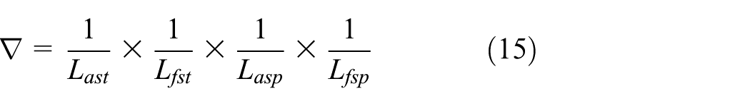
Each link link_ϕ in Tpa is an 1-hop route. The weight of an 1-hop route between node a and node f, denoted as We_af, is defined as follows

$$W{e}_{\mathrm{af}}=\underset{t=1}{\overset{\beta }{\Pi }}\frac{1}{L_{\mathrm{at}}}\times \underset{t=1}{\overset{\beta }{\Pi }}\frac{1}{L_{\mathrm{ft}}}\times \underset{t=1}{\overset{\beta }{\Pi }}\frac{1}{I_{\mathrm{at}}}\times \underset{t=1}{\overset{\beta }{\Pi }}\frac{1}{I_{\mathrm{ft}}}$$

(10)

I_at is the importance coefficient for node a in the tth dimension (t <= β). We use the following equation to calculate the reciprocal of I_at

$$\begin{array}{cc}\multicolumn{1}{c}{\frac{1}{I_{\mathrm{at}}}}& =\frac{\sum _{p=1}^n{E}_{\mathrm{at}}}{E_{\mathrm{at}}}t\in [1,\beta ]\hfill \\ \multicolumn{1}{c}{}& =\frac{\sum _{r=1}^n({{\log }_e}^n\times \frac{H_{\mathrm{ar}}-{H_r}^{min}}{\sum _{p=1}^k{H}_{\mathrm{pr}}-{H_r}^{min}}-1)(\sum _{p=1}^{a-1}{\log }_e^{\frac{H_{\mathrm{pr}}-H_r^{min}}{H_r^{max}-H_r^{min}}}+\sum _{j=a+1}^k{\log }_e^{\frac{H_{\mathrm{jr}}-H_r^{min}}{H_r^{max}-H_r^{min}}})}{\left(({{\log }_e}^n\times \frac{H_{\mathrm{at}}-{H_t}^{min}}{\sum _{p=1}^k{H}_{\mathrm{pt}}-{H_t}^{min}}-1)(\sum _{p=1}^{a-1}{\log }_e^{\frac{H_{\mathrm{pt}}-H_t^{min}}{H_t^{max}-H_t^{min}}}+\sum _{p=a+1}^k{\log }_e^{\frac{H_{\mathrm{pt}}-H_t^{min}}{H_t^{max}-H_t^{min}}})\right)}\hfill \end{array}$$

(11)

I_ft is the importance coefficient for node f in the tth dimension (t <= β). We use the following equation to calculate the reciprocal of I_ft

$$\begin{array}{cc}\multicolumn{1}{c}{\frac{1}{I_{\mathrm{ft}}}}& =\frac{\sum _{p=1}^n{E}_{\mathrm{ft}}}{E_{\mathrm{ft}}}t\in [1,\beta ]\hfill \\ \multicolumn{1}{c}{}& =\frac{\sum _{r=1}^n({{\log }_e}^n\times \frac{H_{\mathrm{ar}}-{H_r}^{min}}{\sum _{p=1}^k{H}_{\mathrm{pr}}-{H_r}^{min}}-1)(\sum _{p=1}^{f-1}{\log }_e^{\frac{H_{\mathrm{pr}}-H_r^{min}}{H_r^{max}-H_r^{min}}}+\sum _{j=f+1}^k{\log }_e^{\frac{H_{\mathrm{jr}}-H_r^{min}}{H_r^{max}-H_r^{min}}})}{\left(({{\log }_e}^n\times \frac{H_{\mathrm{ft}}-{H_t}^{min}}{\sum _{p=1}^k{H}_{\mathrm{ft}}-{H_t}^{min}}-1)(\sum _{p=1}^{f-1}{\log }_e^{\frac{H_{\mathrm{pt}}-H_t^{min}}{H_t^{max}-H_t^{min}}}+\sum _{p=f+1}^k{\log }_e^{\frac{H_{\mathrm{pt}}-H_t^{min}}{H_t^{max}-H_t^{min}}})\right)}\hfill \end{array}$$

(12)

L_at is the ranking value for node a in the tth dimension (t <= β). L_ft is the ranking value for node f in the tth dimension (t <= β).

In our daily life, some dimensions are interrelated; for instance, the past encounter frequency is always related to two dimensions which are the moving speed and the dwell time in a specific location. We use D_afec to represent the past encounter frequency of node a and node f in a specific location. We use L_ast to represent the ranking value of dwell time in the encountering location for node a. We use L_asp to represent the ranking value of the moving speed for node a. We use I_ast to represent the importance coefficient of the dwell time in a specific location for node a. We use I_asp to represent the importance coefficient of the moving speed for node a. In the same way, we use L_fst, L_fsp, I_fst, and I_fsp to represent those values associated with node f. Then if the encounter frequency dimension belongs to those β dimensions but the moving speed dimension and the dwell time dimension do not belong to those β dimensions we use the following equation to calculate the 1-hop route between node a and node f

$$\begin{array}{c}\exists D_{\mathrm{afec}}\in [D_1,D_{\beta }]\forall L_{\mathrm{ast}}\forall L_{\mathrm{fst}}\forall L_{\mathrm{asp}}\forall L_{\mathrm{fsp}}\hfill \\ \{I_{\mathrm{ast}},I_{\mathrm{fst}},I_{\mathrm{asp}},I_{\mathrm{fsp}}\}\notin \{I_{\mathrm{ar}},I_{\mathrm{fr}}\},r\in [1,\beta ]\hfill \\ W{e}_{\mathrm{af}}=\underset{t=1}{\overset{\beta }{\Pi }}\frac{1}{L_{\mathrm{at}}}\times \underset{t=1}{\overset{\beta }{\Pi }}\frac{1}{L_{\mathrm{ft}}}\times \underset{t=1}{\overset{\beta }{\Pi }}\frac{1}{I_{\mathrm{at}}}\times \underset{t=1}{\overset{\beta }{\Pi }}\frac{1}{L_{\mathrm{ft}}}\times \Omega \times \nabla \hfill \end{array}$$

(13)

The equation

$$\Omega =\frac{1}{I_{\mathrm{ast}}}\times \frac{1}{I_{\mathrm{fst}}}\times \frac{1}{I_{\mathrm{asp}}}\times \frac{1}{I_{\mathrm{fsp}}}$$

(14)

And the equation

$$\nabla =\frac{1}{L_{\mathrm{ast}}}\times \frac{1}{L_{\mathrm{fst}}}\times \frac{1}{L_{\mathrm{asp}}}\times \frac{1}{L_{\mathrm{fsp}}}$$

(15)

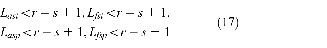
L_at, L_ft, L_ast, L_fst, L_asp, L_fsp are subject to the following constraints

$$L_{\mathrm{at}}\in D_t\cap L_{\mathrm{at}}\ge r-s+1L_{\mathrm{ft}}\in D_t\cap L_{\mathrm{ft}}\ge r-s+1$$

(16)

$$\begin{array}{l}{L}_{ast}<r-s+1,L_{fst}<r-s+1,\\ L_{asp}<r-s+1,L_{fsp}<r-s+1\end{array}$$

(17)

When two nodes meet with each other, they exchange their topology for expansion. Algorithm 4 is used to expand the local topology of node a. Assume that Tpw is the local topology of node w and there are δ links in Tpw, Tpa is the local topology of node a and there are Ü links in Tpa. We use link_ϕ to represent the ϕth link in Tpa. We use link_§ to represent the §th link in Tpw.

Algorithm 4. Pseudo code of expanding local topology executed by node a when encountering node w.
1: Procedure EXPANDTOPO (Tpa, Tpw)
2: a.sendTopologyTo (w)
3: a.getTopologyFrom (w)
4: setϕ = 1
5: for each link linkϕ in Tpado
6:  set§ = 1
7:  for each link link§ in Tpwdo
8:   if (linkϕ.tail node.ID == link§.tail node.ID)
9:    connect(linkϕ, link§)
10:    §++
11:    if (§<=δ)
12:     go on
13:    else
14:     break
15:    end if
16:   else
17:    ϕ++
18:    if (ϕ<=Ü)
19:     go on
20:    else
21:     break
22:    end if
23:   end if
24:  end for
25: end for
26: end procedure

The binary topology of node a is updated after encountering with node f. The topology of node a may be shown as Figures 11 or 12.

Figure 11.

The case 1.

Figure 12.

The case 2.

In Figure 11, there are three shared nodes which can connect Tpa with Tpw. The letters in these nodes are the identification flags. In Figure 12, there are no shared nodes between Tpa and Tpw, and it means there is a partition in the topology of node a. But some nodes that can connect partitions may be encountered and inserted into the topology later. In Figure 11, from node a to node w, there are three routes; we call these three routes l-hop (l > 1) route. The weight of an l-hop route between node a and node w is calculated as follows

$$W_{\mathrm{aw}}=W_{\mathrm{aea}}\times W_{\mathrm{eaw}}+W_{\mathrm{aka}}\times W_{\mathrm{kaw}}+W_{\mathrm{awa}}\times W_{\mathrm{waw}}$$

(18)

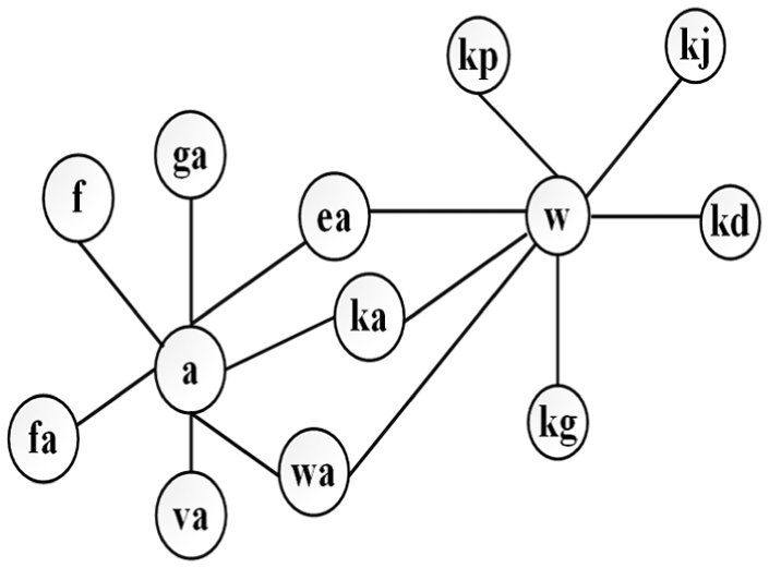
The above algorithms finally generate binary topology that are not identical in all nodes and may not include all nodes. This is similar to our daily lives that each person has his or her own knowledge of the social structure. After warm-up period, assume that the topology of node a is shown in Figure 13.

Figure 13.

The topology of node a after warm-up period.

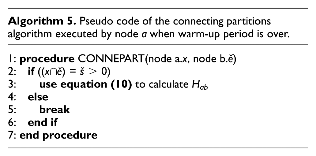
As shown in Figure 13, there are some 1-hop routes and l-hop routes in the topology. For instance, W_aw is the link weight of l-hop route between node a and node w. The dotted line in the topology means that there is no connection between node a and node b. Node a uses the Algorithm 5 to address this issue. Assume that node a ranked in the top s in x (x >= θ) dimensions. Assume node b ranked in the top s in ě (ě >= θ) dimensions.

Algorithm 5. Pseudo code of the connecting partitions algorithm executed by node a when warm-up period is over.
1: procedure CONNEPART(node a.x, node b.ě)
2: if ((x∩ě) = š > 0)
3:  use equation (10) to calculate Hab
4: else
5:  break
6: end if
7: end procedure

Till now, we have constructed the topology of node a, which is dynamic changeable over time, this is because the ranking values of some nodes in the topology will change over time. The topology of node a is also polymorphic; this is because the nodes in topology are diverse over time. Based on the topology, node a can use shortest path algorithm to obtain the optimal relay set, which includes nodes that are on the shortest path for a specific data packet relaying.

As shown in Figure 14, node a sends packet to node eh. Assume that the optimal relay set includes node w, node kg, and node e. If node a encounters one of them, it will send the packet. If node a encounters the three nodes at the same time, the one with a minimal path weight will be selected as the relay node. Till now, we have proposed DR, which utilizes dynamic and polymorphic combination of dimensions to obtain the topology of each node, and then each node can determine the suitable routing based on the topology. Compared with SMART, DR uses more accurate method to define link weight but it suffers from two problems: one is that during the warm-up period, the routing cost of DR is larger than SMART, we can see this result in section “Simulation and evaluation”; another is that DR is also based on the assumption that all nodes in topology have enough energy and cooperate to relay packet. In section “Simulation and evaluation,” when warm-up period is over, compared with SMART, the DR’s advantages is not obvious.

Figure 14.

The example of node a sends packet to node eh.

So in next part, we propose DANCER, which based on dynamic and polymorphic combination of dimensions and energy consideration.

The binary topology construction

In this part, we exploit Nash equilibrium solution to simplify the topology. Assume there are k nodes and the initial energy of each node is shown as follows

$$E_1,E_2,\dots ,E_i,\dots ,E_j,\dots ,E_k\forall i,j\in [1,k]E_i\ne E_j$$

(19)

Assume energy consumption for sending a specific packet is

$$E_{1s},E_{2s},\dots ,E_{\mathrm{is}},\dots ,E_{\mathrm{js}},\dots ,E_{\mathrm{ks}}\forall i,j\in [1,k]E_{\mathrm{is}}\ne E_{\mathrm{js}}$$

(20)

Assume energy consumption for relaying a specific packet is

$$\begin{array}{c}{E}_{1t},E_{2t},\dots ,E_{\mathrm{it}},\dots ,E_{\mathrm{jt}},\dots ,E_{\mathrm{kt}}\hfill \\ \forall i,j\in [1,k]E_{\mathrm{it}}\ne E_{\mathrm{jt}},E_{\mathrm{it}}>E_{\mathrm{is}}\forall i\in [1,k]\hfill \end{array}$$

(21)

Assume payoffs for sending a specific packet is

$$B_{1s},B_{2s},\dots ,B_{\mathrm{is}},\dots ,B_{\mathrm{js}},\dots ,B_{\mathrm{ks}}\forall i,j\in [1,k]B_{\mathrm{is}}\ne B_{\mathrm{js}}$$

(22)

Assume payoffs for relaying a specific packet is

$$B_{1t},B_{2t},\dots ,B_{\mathrm{it}},\dots ,B_{\mathrm{jt}},\dots ,B_{\mathrm{kt}}\forall i,j\in [1,k]B_{\mathrm{it}}\ne B_{\mathrm{jt}}$$

(23)

For a certain link in topology, assume that node i and node j are the endpoints associated with the link. Based on the Game theory, we define the payoff matrix which associates with node i and node j is

$$\begin{array}{c}\mathrm{node}j\hfill \\ \mathrm{node}i\left[\begin{array}{ccc}(U_i,U_j)\hfill & (V_i,V_j)\hfill & (W_i,W_j)\hfill \\ \multicolumn{1}{c}{(X_i,X_j)}& (Y_i,Y_j)\hfill & (Z_i,Z_j)\hfill \\ \multicolumn{1}{c}{(O_i,O_j)}& (P_i,P_j)\hfill & (Q_i,Q_j)\hfill \end{array}\right]\hfill \end{array}$$

(24)

The U_i in (U_i, U_j) represents the total payoffs of node i for sending a specific packet and relaying packet from its prior node. The U_j in (U_i, U_j) represents the total payoffs of node j for sending a specific packet and relaying packet from its prior node. They are calculated as follows

$$\left(U_i,U_j\right)=(B_{is}+B_{it}+E_i-E_{is}-E_{it},B_{js}+B_{jt}+E_j-E_{js}-E_{jt})$$

(25)

The V_i in (V_i, V_j) is the same as U_i. The V_j in (V_i, V_j) represents the total payoffs of node j for sending packet but not relaying packet from its prior node. They are calculated as follows

$$(V_i,V_j)=(B_{\mathrm{is}}+B_{\mathrm{it}}+E_i-E_{\mathrm{is}}-E_{\mathrm{it}},B_{\mathrm{js}}+E_j-E_{\mathrm{js}})$$

(26)

The W_i in (W_i, W_j) is the same as U_i. The W_j in (W_i, W_j) represents the total payoffs of node j for not sending packet and not relaying packet from its prior node. They are calculated as follows

$$(W_i,W_j)=(B_{\mathrm{is}}+B_{\mathrm{it}}+E_i-E_{\mathrm{is}}-E_{\mathrm{it}},E_j)$$

(27)

The X_i in (X_i, X_j) represents the total payoffs of node i for sending packet but not relaying packet from its prior packet. The X_j in (X_i, X_j) is the same as U_j. They are calculated as follows

$$(X_i,X_j)=(B_{\mathrm{is}}+E_i-E_{\mathrm{is}},B_{\mathrm{js}}+B_{\mathrm{jt}}+E_j-E_{\mathrm{js}}-E_{\mathrm{jt}})$$

(28)

The Y_i in (Y_i, Y_j) is the same as X_i. The Y_j in (Y_i, Y_j) is the same as V_j. They are calculated as follows

$$(Y_i,Y_j)=(B_{\mathrm{is}}+E_i-E_{\mathrm{is}},B_{\mathrm{js}}+E_j-E_{\mathrm{js}})$$

(29)

The Z_i in (Z_i, Z_j) is the same as X_i. The Z_j in (Z_i, Z_j) is the same as W_j. They are calculated as follows

$$(Z_i,Z_j)=(B_{\mathrm{is}}+E_i-E_{\mathrm{is}},E_j)$$

(30)

The O_i in (O_i, O_j) represents the total payoffs of node i for not sending packet and not relaying packet from its prior node. The O_j in (O_i, O_j) is the same as X_j. They are calculated as follows

$$(O_i,O_j)=(E_i,B_{\mathrm{js}}+B_{\mathrm{jt}}+E_j-E_{\mathrm{js}}-E_{\mathrm{jt}})$$

(31)

The P_i in (P_i, P_j) is the same as O_i. The P_j in (P_i, P_j) is the same as V_j. They are calculated as follows

$$(P_i,P_j)=(E_i,B_{\mathrm{js}}+E_j-E_{\mathrm{js}})$$

(32)

The Q_i in (Q_i, Q_j) is the same as O_i. The Q_j in (Q_i, Q_j) is the same as W_j. They are calculated as follows

$$(Q_i,Q_j)=(E_i,E_j)$$

(33)

The payoffs of each node are different so based on the payoffs matrix, they can use Nash equilibrium solution to simplify the topology for a specific packet sending.

The complexity of Algorithm 6 is O(Ü); Ü is the number of links in the topology of node a. Once the simplifying process is done, node a can obtain one of five different topology.

Algorithm 6. Pseudo code of the topology simplification algorithm executed by node a upon sending a packet to node y.
1: procedure TOPOSIMPLIFY (Tpa)
2: setϕ = 1
3: for each link linkϕ in Tpado
4:  if ((node i.energy is Shortage OR node i.packet queue is Full) OR (node j.energy is Shortage OR node j.packet queue is Full))
5:   linkϕ.flag bit == 0
6:  else
7:   build the payoffs matrix
8:   if (Nash Equilibrium solution == (Ui, Uj))
9:    linkϕ.flag bit == 1
10:   else
11:    linkϕ.flag bit == 0
12:   end if
13:  end if
14:  ϕ++
15:  if (ϕ < Ü)
16:   go on
17:  else
18:   break
19:  end if
20: end for
21: end procedure

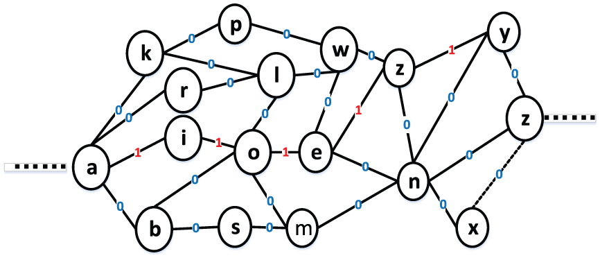
In Figure 15, it shows the binary topology of node a in the first case. The binary topology is composed of links where flag bits are 1 or 0. The link where flag bit is 1 represents that it is useful for a specific packet relaying. For instance, node a sends packet to node y, as we can see there are two paths from node a to node y, without running the Shortest Path algorithm, node a only need to select the shorter path, the complexity to determine packet forwarder is O(x) (x is an integer). Besides, the links where flag bits are 1 compose a Graph like data structure.

Figure 15.

The first case.

Figure 16 demonstrates the binary topology of node a in the second case. The links where flag bits are 1 compose a Linear like data structure. There is only one path from node a to node y. The complexity to determine packet forwarder is O(x) (x is an integer).

Figure 16.

The second case.

Figure 17 shows the binary topology of node a in the third case. The links where flag bits are 1 compose a Tree like data structure. There is only one path from node a to node y. The complexity to determine packet forwarder is O(x) (x is an integer).

Figure 17.

The third case.

Figure 18 shows the binary topology of node a in the fourth case, which is the undesirable case since all the link flag bits are 0. We need another strategy to address this issue in future work (i.e. the incentive policy).

Figure 18.

The fourth case.

Figure 19 demonstrates the binary topology of node a in the fifth case; all the links are useful for packet relaying. There are multiple paths from node a to node y, and node a need to run the shortest path algorithm; the complexity to determine packet forwarder is O(z²) (z is the number of nodes in Tpa).

Figure 19.

The fifth case.

The binary topology of each node is constructed based on the Nash equilibrium solution, and it can avoid some unnecessary energy consumptions when sending or relaying packets. To be specific, each two nodes in topology construct their payoff matrix based on the energy consumptions and payoffs for sending or relaying a specific packet and then they obtain the Nash equilibrium solution to decide whether to send or relay the packet. Therefore, the total routing cost in DTN can be saved by this way. The effectiveness of using Nash equilibrium solution will be evaluated in section “Simulation and evaluation.”

Assume path_af represents the path from node a to node f in Tpa. Assume set_ops is the optimal relay set for node a send packet to node f.

Once Algorithm 7 is done, node a can obtain the set_ops which is used for sending packet to node f. Then the sending pointer points to the next packet in sending queue of node a. Node a utilizes Algorithm 8 to clear the flag bits where are 1. Assume the number of links, where flag bits are 1, is µ. We use a link set Spl to represent the links where flag bits are 1.

Algorithm 7. Pseudo code of the finding optimal relay set algorithm executed by node a upon sending a packet to node y.
1: Procedure FINDODS (Tpa)
2: if ((pathaf is tee like) OR (pathaf is linear
like))
3:  setops = all nodes in pathaf
4: else
5:  LaunchShortestPathAlgFor(y)
6: end if
7: end procedure

Algorithm 8. Pseudo code of the clearing flag bits algorithm executed by node a.
1: procedure CLEARINGFLAGBITS (Tpa)
2: for each linkθ in Spldo
3: setθ = 1
4: if (linkθ.flag bit == 1)
5:  setlinkθ.flag bit == 0
6:  θ++
7:  if (θ < µ)
8:   go on
9:  else
10:   break
11:  end if
12: end if
13: end for
14: end procedure

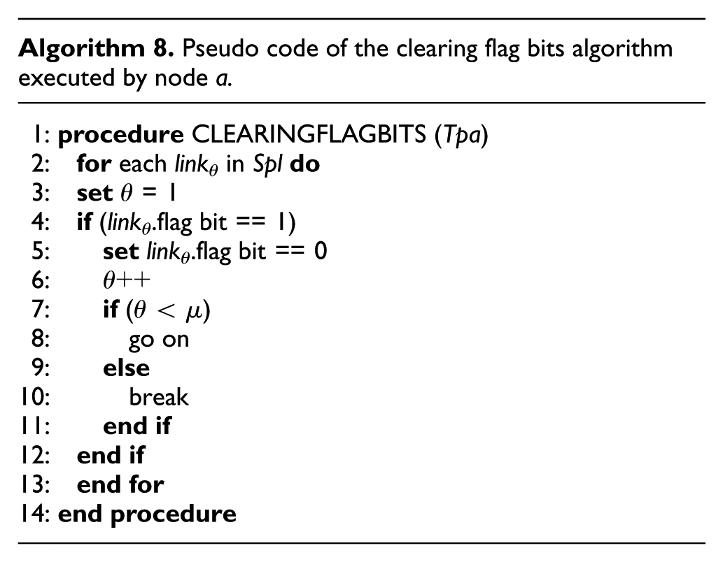
Once Algorithm 8 is done, Algorithm 9 is used to update the initial energy of the nodes which in set_ops. Assume there are ě nodes in set_ops. Assume Š as the counting variable. Assume E_Ši as the initial energy of the Šth node in set_ops. Assume E_Šs as the energy consumption of sending a packet. Assume E_Št as the energy consumption of relaying a packet. Assume B_Šs as the payoffs of sending a packet. Assume B_Št as the payoffs of relaying a packet.

Algorithm 9. Pseudo code of the initial energy updating algorithm executed by node a.
1: Procedure ENERGYUPDATE (setops)
2: for each node in setopsdo
3:  setŠ = 1
4:  EŠ = EŠi-EŠs-EŠt+BŠs+BŠt
5:  Š++
6:  if (Š < ě)
7:   go on
8:  else
9:   break
10:  end if
11: end for
12: end procedure

Algorithm 10. Pseudo code of the DANCER routing algorithm executed by node a.
1: Procedure DANCER (Tpa, Qa)
2: for each packet Py in Qado
3:  set y = 1
4:  if (Py.TTL == 0)
5:   drop Py
6:  else
7:   Launch Algorithm 6 to simplify Tpa
8:   Launch Algorithm 7 to obtain the setops
9:   if ((the encounter node∈setops) AND (the encountered node not receive the Py before))
10:    send Py to the encountered node
11:   else
12:    keep Py and wait for a better chance
13:   end if
14:    Launch Algorithm 8 to clear the flag bits
15:    Launch Algorithm 9 to update the initial energy of each node in setops
16:    y++
17:   if (y < p)
18:    go on
19:   else
20:    break
21:   end if
22:  end if
23: end for
24: end procedure

Based on the previous work, in the next part, we will introduce the DANCER routing algorithm.

DANCER routing algorithm

Assume that there is a packet queue Q_a in node a and the number of packets in Q_a is p. Set P_y is the yth packet in Q_a.

Simulation and evaluation

Simulation setup

In this part, we conduct simulations to evaluate the effectiveness of DANCER and compare it against five other DTN routing schemes (Epidemic, SimBet, Prophet, DR, and SMART). The simulations are carried out using the OMNET++ simulator,^22,23 which is driven by discrete event and used to evaluate the performance of routing scheme for DTN; it is also an open-source simulator allowing to create mobile models upon different synthetic movement and real-life traces. The node mobility of our simulation is based on the Massachusetts Institute of Technology (MIT) reality trace file,^21,24 which consists of the mobility information of 97 users with Nokia 6600 mobile phone in MIT campus during the 2004–2005 academic year; thus, it can provide information about contact event.

In order to reflect the dynamic combination of dimensions, we select four observation periods from the MIT trace file for simulation and we use five attributes from the MIT reality trace file including moving speed, location, occupation, contact frequency, and hobby to represent five dimensions. However, the MIT reality data set does not provide location information of node movement, but this drawback had been overcome by Ficek and Kencl. ²¹ Moreover, the MIT reality data set does not provide moving speed information either, so we address it using random number generation function to generate 90 random numbers as the moving speed of each node in our simulation. We randomly select three out of five dimensions to be used in four different simulation periods. In our simulation, we set 90 nodes that are randomly correspondence to 90 users in MIT reality trace file; the total simulation period is five working days. The first working day is selected as a warm-up period to construct the initial binary topology without any packet created during this period. Then the nodes are randomly selected to be the source or destination and some of the packets between the number of 5 and 500 were created. In simulation period 1, the node mobility is based on the trace file from 2004-10-1 to 2004-11-1. In simulation period 2, the node mobility is based on the trace file from 2004-11-1 to 2004-12-1. In simulation period 3, the node mobility is based on the trace file from 2004-12-1 to 2005-1-1. In simulation period 4, the node mobility is based on the trace file from 2005-1-1 to 2015-2-1. Using the random number generation function, we generate 270 random numbers to represent 90 initial energy, 90 energy consumption, and 90 payoffs of each node. The detail simulation parameters are shown in Table 1. Three metrics are focus in simulations:

• Routing energy cost: the total relaying energy consumption in simulation.

• Successful delivery ratio: the ratio of packets received by the destination from those generated by the source.

• Average delay: the average time interval among the sending and receiving events for packets traveling along the network.

Table 1.

Simulation parameters.

Parameter	Value
Installation environment	Ubuntu-14.04.5
Simulator	OMNET++
The number of nodes	90
Buffer size	400–3600 KB
Number of generated packets	5–500
The size of each packet	0.1 (KB)
The initial energy of each node	90 random numbers
The energy consumption of sending a packet	90 random numbers
The energy consumption of relaying a packet	90 random numbers
The payoffs of sending a packet	90 random numbers
The payoffs of relaying a packet	90 random numbers
Warm-up period	8 h
Simulation period 1	8 h
Simulation period 2	8 h
Simulation period 3	8 h
Simulation period 4	8 h

Simulation results and analysis

In this part, we evaluate how the successful delivery ratio, the average delivery delay, and the routing cost of the six routing schemes will change under the following conditions: (1) the TTLs of the messages, (2) the buffer size, and (3) the number of the generated packets.

Performance with different TTLs of packets

Successful delivery ratio

Figure 20 demonstrates the successful delivery ratio of the six routing schemes with the MIT reality trace. From the figures, we see that the successful delivery ratio of the six schemes follow DANCER > DR > SMART > PROPHET > SIMBET> EPIDEMIC.

Figure 20.

The successful delivery ratio with different TTLs.

We observe that as the TTLs of the packets increase, the delivery ratio of six schemes increase. EPIDEMIC shows the lowest successful delivery ratio, while DANCER shows the highest by deducing nodes’ delivery abilities to destinations based on the binary topology, so that it can choose an optimal forwarder in a comprehensive way. It is showed that the two curves of DR and SMART are close; the first reason is that DR does not have energy consideration; the second is that in our simulation, DR just uses three dimensions to define the link weight, so that it does not have much advantage to SMART. PROPHET and SIMBET can only evaluate the delivery ability within one or two hops, which cannot consider long routing paths, leading to a lower delivery ratio than DANCER, DR, and SMART.

Average delay

Figure 21 shows the average delay of six schemes in the tests with the MIT reality. From the figure, we find that the average delay of six schemes follows EPIDEMIC > PROPHET > SIMBET > SMART > DR > DANCER. DANCER has the lowest average delay because it uses the binary topology, which enables a packet to travel through a fast route to its destination. While the EPIDEMIC has the highest average delay. As we can see in the figure, when the TTLs between 0 and 23, the average delay of DR is lower than SMART, but when TTLs between 23 and 31, the average delay of SMART is lower than DR; the reason is that DR is based on the assumption that all nodes are cooperate to relay packets and DR uses three dimensions to define the link weight, so it could not show the obvious discrepancy between the two curves. Both PROPHET AND SIMBET fail to consider long paths that may generate shorter delay. Therefore, they produce higher average delay than DANCER, DR, and SMART.

Figure 21.

The average delay with different TTLs.

Routing cost

Figure 22 shows a plot of the routing cost of six schemes with the MIT reality trace. From the figure, we see that EPIDEMIC has the highest routing cost since it is the flooding-based strategy. DANCER incurs a significant lower routing cost than other five schemes, this is because two encountered node uses the binary topology, which consider both multiple dimensions and energy. SIMBET has a slightly higher routing cost than PROPHET since in addition to the similarity information; a node has to send its centrality information to the newly met node. DR has a slightly higher routing cost than SMART, this is because DR uses three dimensions while SMART uses one dimension, so when nodes exchange information, DR can cause more energy consumption.

Figure 22.

The routing cost with different TTLs.

Performance with different buffer sizes

Successful delivery ratio

Figure 23 shows the successful delivery ratios of six schemes with the MIT reality trace when the buffer size varies. We see that the successful delivery ratios of six schemes follow the same as in Figure 20 due to the same reasons. We also find that when the buffer size on a node increases, the hit rates of all schemes also increase. This is because with larger buffer size, each node can carry and forward more packets to their destinations, leading to a high delivery ratio.

Figure 23.

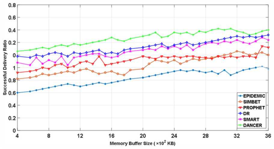
The successful delivery ratio with different buffer sizes.

Average delay

Figure 24 shows the average delay of the six schemes with the MIT reality trace when the buffer size on each node varies. We find that the relationship of the six schemes on the average delay is the same as in Figure 21 for the same reason. It is interesting to see that when the buffer size on a node increases, the average delays decrease. This is because when the buffer size increases, there are fewer dropped packets, whose delay is very large, leading to decreased average delay.

Figure 24.

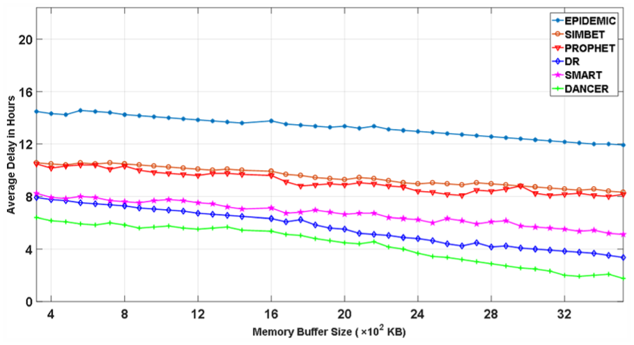
The average delay with different buffer sizes.

Routing cost

Figure 25 demonstrates the routing cost of the six schemes with the MIT reality trace when the memory size on each node varies. We find that the routing cost almost is the same as in Figure 13(c) for the same reason. We can see in the figure, DANCER has always maintained lower energy consumption. Although both DANCER and DR consider the dynamic combination of multiple dimensions, DANCER further consider the selfishness of nodes while DR ignores about this and it is based on the assumption that all nodes in topology are cooperated to relay the packets. The result of that brings some unnecessary energy consumption, as shown in Figure 26.

Figure 25.

The routing cost with different buffer sizes.

Figure 26.

Example of the unnecessary energy consumption.

Node a sends a packet to node b and it thought node b is the ideal packet forwarder, but it does not take the selfishness of node b into consideration, the result of that is node b may refuse to accept the packet or accept the packet but drop it. Thus, it will increase the total energy consumption of routing. Different from other five strategies, DANCER uses Nash equilibrium solution in advance to determine whether to send the packet to the encountered node, so that DANCER will save some energy.

Performance with different numbers of packets

Successful delivery ratio

Figure 27 shows the successful delivery ratios of six schemes with the MIT reality trace when the number of packets varies. We see that the successful delivery ratios of six schemes follow the same as shown in Figure 20 due to the same reasons. We also find that when the number of packets increases, the delivery ratio of all schemes decreases. This is because with larger number of packets, each node has limited buffer size, leading with some packets dropped.

Figure 27.

The successful delivery ratio with different numbers of packets.

Average delay

Figure 28 shows the average delay of the six schemes with the MIT reality trace when the buffer size on each node varies. We find that the average delay of the six schemes follow EPIDEMIC> (PROPHET, SIMBET) > (DR, SMART) >DANCER. DANCER has the lowest average delay due to the same reason in Figure 21. It is interesting to see that the curve of SMART and DR are almost overlapped. This is because when the buffer size and TTLs are fixed, the average delay of DR is almost equivalent to SMART due to the same reason in Figure 21. We can also see when the number of packets increases, the average delays of six schemes increase. This is because when the buffer size is fixed; there will be more dropped packets that leading to increase average delay.

Figure 28.

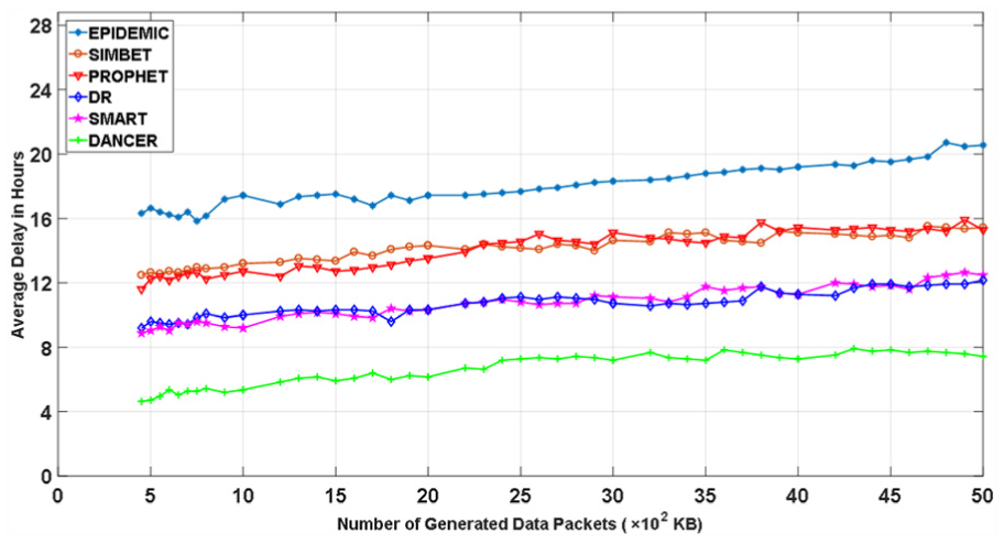
The average delay with different numbers of packets.

Routing cost

Figure 29 demonstrates the routing cost of the six schemes with the MIT reality trace when the number of packets varies. We find that the routing costs are almost the same as in Figure 22 for the same reason. In the figure, DANCER has always maintained lowest energy consumption while EPIDEMIC has the highest routing cost. It is interesting to see that the curve of PROPHET and SIMBET are almost overlapped. This is because when the buffer size is fixed, the routing performance of PROPHET is almost equivalent to SIMBET. Besides, DR has slightly higher routing cost than SMART due to the same reason in Figure 22.

Figure 29.

The routing cost with different numbers of packets.

When we use the fuzzy comprehensive evaluation of the fuzzy mathematics ²⁵ to evaluate the routing impact parameters, we find that the buffer size has a large effect on routing performance. So in our simulation, we fix the TTLs and the number of generated packets. In order to observe the affection of the number of dimensions to the routing performance, we set different numbers of dimensions (i.e. 4, 6, 8) used in DANCER. Furthermore, we do not use DR for comparison in this simulation. Figures 30–32 demonstrate the delivery ratio, the average delay, and the routing cost of the seven schemes with MIT reality trace when the buffer size varies, respectively. We find that the delivery ratios of the seven schemes follow DANCER (n = 8) > DANCER (n = 6) > DANCER (n = 4) > SMART> SIMBET > PROPHET > EPIDEMIC. The average delay of the seven schemes follows EPIDEMIC > SIMBET > PROPHET > SMART >DANCER (n = 4) > DANCER (n = 6) >DANCER (n = 8); the above results are because the more number of dimensions is used in DANCER, the more accurate route will be defined, which leads to a better delivery ratio and average delay. For routing cost, it is interesting to see that three curves with different numbers of dimensions are overlapped, which contrary to our expected experiment results. We suppose the reason for the following points: the first reason is that in our simulation, we can only accurately extract five dimensions from the MIT data set. The second reason is that due to our limited knowledge about the dimensions mining algorithm, if more than five dimensions are extracted, there will be some intersection between dimensions.

Figure 30.

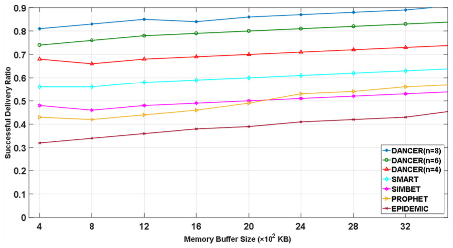
The successful delivery ratio with different numbers of dimensions.

Figure 31.

The average delay with different numbers of dimensions.

Figure 32.

The routing cost with different numbers of dimensions.

Conclusion and future works

In this article, we propose DANCER, which is a novel routing algorithm in DTNs that utilizes binary topology on mobile node. By exploiting the similarity in multiple dimensions, DANCER enables each node to construct a topology to record its knowledge of surrounding structure. Specifically, nodes in topology are ranked in top s in multiple dimensions; the link weights in topology are defined by the reciprocals of the node’s ranking values in multiple dimensions and the reciprocals of importance coefficients of each dimension. Based on the topology, DANCER enables each node to use Nash equilibrium solution to obtain a binary topology for labeling the links that can be used to relay packets, so that each node can determine the suitable routing. The dynamic reflected in the topology of each node is changeable over time, due to the ranking value of each node in different dimensions changes over time. The polymorphic of binary topology is not only reflected in the changeable number of nodes or nodes’ IDs, but also reflected in the changeable flag bits when sending diverse packets. The simulation experiment demonstrates the effectiveness of DANCER in comparison to previous algorithms.

For future work, we intend to utilize fuzzy set division of fuzzy mathematics ²⁵ to reasonably divide the rank number of each dimension. Moreover, enlightened by the community mining method^26,27 used in complex networks, the communities in complex networks are correspond to the dimensions mentioned in our article, and the communities’ overlapping can be considered as the intersection between dimensions. So in the future, we will also study the dimension mining algorithm, which means utilize the knowledge of data mining to extract more accurate dimensions.