
Abstract
In this study, an innovative distributed method for achieving external clock synchronization is presented. Based on discrete-time clock models, it can realize synchronization of clocks while enabling their time to change at the same pace simultaneously. Stronger robustness against noisy measurements and clock rate drifts is gained by combining both controller and estimator design methods into the protocol. Additionally, a specifically designed communication scheme is proposed to make our protocols independent on global physical time. To render our protocols more practical, the control variable for clock synchronization is ensured bounded and a stopping criterion for implementation of the protocols is established. Finally, performance of the method is illustrated by certain numerical simulations.
Introduction
Technological advancement of low-cost and low-power programmable sensors has been witnessed during these years. These sensors are capable of sensing, recording, and processing data, as well as communicating via wireless channels. They can be distributed in large areas to monitor physical phenomena, making up wireless sensor networks (WSNs). In WSNs, sensor nodes can be embedded in the environment to be static, or they are enabled to be mobile with physical artifacts carrying them. 1
WSNs are closely coupled to application backgrounds. 2 Climate monitoring, target positioning, and event detection are time-critical applications in which local clocks of all sensors must have the same time value. However, oscillators in low-cost sensors result in different local clock time with distinct drifting speed. Thus, clock synchronization is a significant and interesting topic attracting focuses of many researches. Although successful clock synchronization protocols for wired networks have been developed for decades, they are inappropriate for WSNs for facts that WSNs have a wider deployment, constraint power supply, and a higher demand on robustness.
Literature review
For clock synchronization in WSNs, it includes the following method patterns: 3 master-to-slave versus peer-to-peer synchronization. Master-to-slave protocols, among which we will list some to review, assign certain nodes as masters. Reference Broadcast Sync seeks to reduce non-deterministic time delay using partial aggregations and conserves energy via the post facto scheme. 4 However, it has to divide the network into multiple clusters and choose master nodes for each cluster, which increases workloads of communication and computation. Time-Diffusion Sync Protocol 5 utilizes a diffusion of messages, in which all nodes participate to establish network-wide balanced time. A radial tree structure is formed with an election and re-election cycle where each node decides to become a master or a diffused-leader on its own. With the structure, an iterative weighted-averaging process can be carried out. Timing-sync Protocol for Sensor Networks (TPSN) 6 builds up a spanning tree along whose branches pair-wise synchronization is executed by sender–receiver handshake 7 exchanges, before the phase of synchronization. Master-node failure is a common problem with which these methods are confronted. In another method called Flooding Time Sync Protocol, receiving nodes record incoming time-stamps’ arrival instants and normalize them, after which they update their own time-stamps and then broadcast them to their neighbors. 8 This method achieves robustness to root failure to some extent, but not completely.
Compared with master-to-slave protocols, peer-to-peer protocols are distributed without center nodes. Then, problems caused by master-node failure do not exist. Average Time Sync (ATS) 9 utilizes a cascade of two consensus algorithms to achieve the consensus of clock skews and that of offsets separately by tuning compensation parameters. In Distributed Time Sync, 10 neighboring nodes exchange time-stamp packets on a one-to-one basis. Any participating node can become a reference node by simply not adjusting its own clock during the synchronization procedure, which converts synchronization into solving an optimization problem. To obtain faster convergence and better energy efficiency, Clustered Consensus Time Synchronization (CCTS) 11 combines the Distributed Consensus Time Synchronization (DCTS) algorithm with the clustering technique. However, it still compensates skew and offset parameters separately and requires additional energy for clustering.
However, method patterns can be roughly classified into internal versus external synchronization. The physical-clock rate which depends on the oscillator frequency usually cannot be tuned directly, while external time of local clocks can be synchronized more easily. 12 Thus, external clocks, also called virtual clocks, can be modeled to make synchronization much easier. However, only certain literature, such as CCTS 11 and FLOPSYNC-2, 13 presents relatively specific relationships between actual and virtual clocks.
Statement of contribution
Compared with previous research work, our article contributes to the following innovations as far as we know:
Unlike most previous literature, 14 clock skews of sensor nodes in our method can be time-varying, which makes the model more apposite in implementation.
Synchronization of clock rates and that of initial local time are achieved separately by most works9,15 with several coupled algorithms. However, on one hand, this separation can result in slower convergence, which means heavy burdens of communication and computation. On the other hand, performance of coupled algorithms would interact with each other, which may have an undesirable accumulated effect on synchronization precision. Like certain literature, 16 our method combines and solves these two tasks jointly to achieve external synchronization with light-weight linear protocols.
Inspired by both controller and estimator design methods, our protocol combines their advantages as in the literature9,13 to follow drifts of clock time with noise filtering. Besides, control inputs used to adjust time of local clocks are proved to be bounded, which was rarely considered by previous researches.
Certain application details usually omitted in theoretical researches are considered and explained in this article. First, the virtual-time model is clearly distinguished from the physical-clock model to make this external synchronization more applicable. Then, a specifically designed communication scheme is proposed to explicitly show how sensor nodes execute packets’ receiving and transmitting with absence of global time information. Meanwhile, inspired by literature, 9 the communication scheme is modified to expand its application with asynchronous communication.
A stopping criterion for our synchronization protocols is established in a distributed way. Then, the synchronization process can be ended in finite time, which is significant in practical implementation.
Notation and graph theory
Notation
For a number
Graph theory
An undirected graph
An extended neighbor graph, denoted as
For a graph

Clock models and proposed synchronization protocols
Problem formulation
First, one classical simplified clock-time model 18 can be presented as

where
When
Since
Synchronization of local time and that of local time variations should be achieved simultaneously for the sake of synchronization accuracy and power conservation.
In this article, we explain how we try to solve the above concerns.
Models and protocols
Continuous clock synchronization poses a high demand for power supply, which is not practical for WSNs. So, we establish a discrete-time sampling model of each local clock as

where

Schematic diagram of communication between node 1 and its neighbors.
However, there are reasons that prevent us from utilizing this physical sampling model directly. First, it is not practical to adjust oscillators or counters of these sensors which may be deployed in inaccessible or atrocious environments. Additionally, this discrete-time form has the implicit disadvantage of causing time discontinuity, which may lead agents to making unexpected faults such as missing significant events or recording the same thing multiple times. These critical issues are usually omitted by methods for internal synchronization.
As a solution to above problems, a model of virtual local clock whose time can be directly tuned by a control input is established. Virtual-clock synchronization only needs achieving for cooperative events requiring for common time. And physical clocks, which are referred to for individual time events, still work due to their own mechanical schemes. On

where
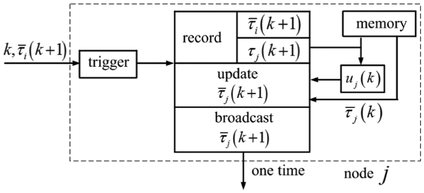
Schematic diagram of packets’ recording and broadcasting.
Thus, synchronization can be achieved by designing protocols for

where

where
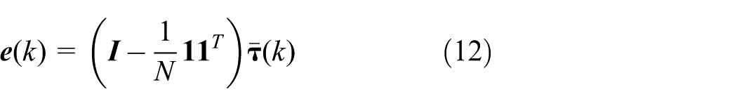
The vector form of above expressions can be expressed as

where
Due to this assumption,

from which it can be seen that the effect of noise mainly from
However, we utilize the transfer function method by taking


Scheme of the feedback control system.
In this way, equation (5) can be converted into a feedback control system which is linear and time-invariant without uncertainty and model errors. Then, its closed-loop transfer function can be figured out as

which shows the stability of this control system. Thus, as long as messages are exchanged regularly enough, the input of this system is bounded, which ensures
After the above analysis, we take the design of

where

where

where
Then, one Lyapunov function can be established in the following form

Using the definition of

where

equates with
Stability and consensus achieving analysis
Stability here means the input-to-state stability (ISS) of the whole system, which can ensure virtual time of all nodes to have bounded values respectively, while consensus represents that all bounded stable values of the virtual time converge to the same one asymptotically.

where

where

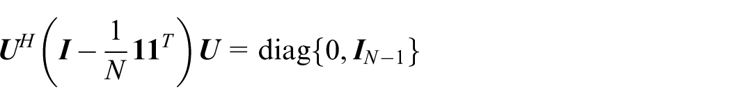
Let

which can be transformed to the decoupled vector form as

The component-wise form of it is
With values of

Then, Schur stability can be achieved by utilizing the Jury stability criterion directly. According to the criterion, a test chart needs tabulating as Table 1 first,
Chart of Jury stability criterion.

where
Then, following constraints

have to be satisfied according to the criterion. Therefore, the value range of
When parameters are chosen within the ranges mentioned above, all eigenvalues of the system matrix are included in a unit circle, that is, the system matrix is Schur-stable. Then, values of all state vectors in the state-space expression are bounded, depending on the bounded values of inputs due to ISS. 19 Therefore, the whole system achieves stability. Till now, the proof is completed.

where
asymptotically under the presented protocols.

Then, for all nodes, its vector form is
which implies that the average consensus of

Due to the fact that
Thus, by letting

which infers

This implies that
Then, the fact obtained in the previous subsection that
Combining these two expressions yields

Then with
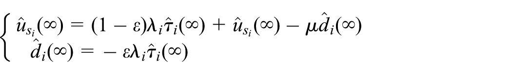
To make the virtual common-time value more explicit, the case
By recursion of above expressions,

As a constant factor of k,
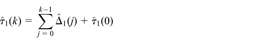
Due to the following process of inference

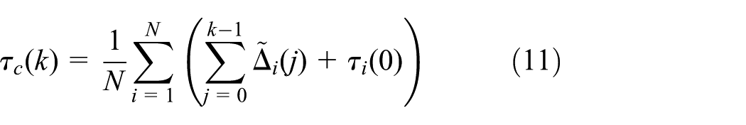
the value of virtual common time can be denoted as

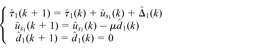
Besides, when clock skews are constant, consensus of local time variations also means consensus of local clock skews. In this case, it is easy to figure out that
Then, equation (14) can be transformed to

Let
Implementation
Communication scheme
In this subsection, certain detailed attributes of the communication scheme presented in Remark 1 are supplemented. That communication means can be summarized as a reactive flooding scheme with the MAC-layer time-stamping. The MAC-layer technique does not only have the function mentioned in Remark 1, but also has the function of preventing transmission collisions. Specifically, message transmission between two nodes does not interfere with transmission between other nodes. Reactive, similar with the term post facto in RBS, 4 represents that sensor nodes are triggered to find communication links instead of getting routing information known and stored proactively. This attribute leads to energy savings for the fact that no energy is consumed for attempting to maintain routines at all time. The flooding scheme has been explained in Remark 1. By flooding, packets are transmitted only over multiple short distances between pairs of neighbors instead of a single long path, which reduces energy consumption.
Application with asynchronous communication
Modified communication scheme
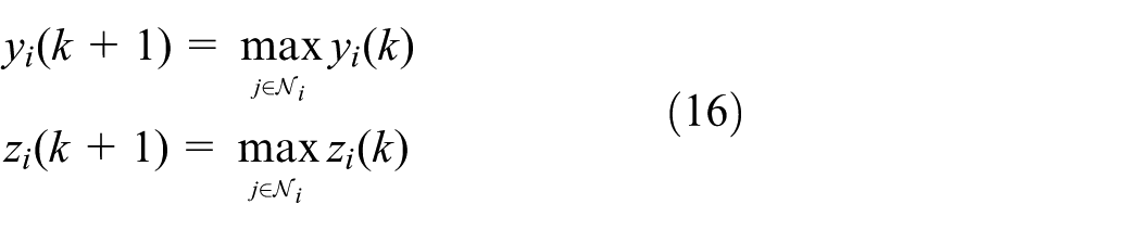
In WSNs, if message channels are full duplex, the communication graph can be connected undirected due to Assumption 2. However, in most cases of WSNs, sensor nodes cannot transmit packets immediately when they receive packets. That is to say, these channels are half-duplex, which implies that underlying communication graphs on sampling instants are unidirectional. Here, it is worth reminding that the message-channel graph of the whole net is still connected undirected. Then, the communication scheme in Remark 1 has to be modified so as to be applicable in this case. Node i updates its own virtual time-stamp immediately when it records its local physical time, which is triggered by receiving the incoming packet from node j. This event’s global instant is denoted as
Now let
Comparison to existing methods
Compared with existing ideas of implementation,
9
our method of addressing the asynchronous problem is more practical. Actually, Schenato and Fiorentin
9
implicitly assume that one of the following two conditions has to establish when its implementation method is applied. One is that all nodes start the synchronization on the same global instant. The other is that all physical-clock skews are constant. However, both conditions are not practical due to the problem formulation. Specifically, a counter-example is shown in Figure 4, where there are four nodes making up the net. From the literature,
9

A counter-example of the existing implementation method.
As for the method proposed in this article, from subsection “Modified communication scheme,”
Stopping criterion for synchronization protocols
Though it has been proven that clock synchronization can be achieved asymptotically, Pottie and Kaiser 21 show that a considerable amount of energy has to be conserved in practice by finishing the synchronization process in finite time. Yadav and Salapaka 22 has proved that average-consensus protocols whose underlying graphes are undirected or strongly connected balanced can be ended in finite time by designing minimum and maximum consensus protocols.
Since synchronization of clock time and that of time variations are achieved simultaneously, our stopping criterion is to utilize virtual-time variations. Thus, the protocols are designed as
where
After all nodes stop exchanging messages and running protocols for synchronization, they can return to low-power states to save energy. Then a whole strategy for clock synchronization is accomplished.
Numerical simulations
In this section, performance of proposed protocols is illustrated by presenting certain simulation results.
We consider three examples of WSN grids consisting of 6 nodes, 36 nodes, and 800 nodes, respectively, for two main reasons. On one hand, the scalability of our proposed method can be illustrated when the scale of the network differs. On the other hand, details that may not be seen clearly in the figure of a large net can be displayed explicitly in the figure of a small net.
Above all, Figure 5 shows the underlying graphs of nets with different scales, on which our simulation is carried. It can be seen from the figure that all graphs are connected undirected. Figure 6 shows how local time of all nodes in Figure 5 changes corresponding to the physical time before synchronization. In the figure, curves with different colors represent local clocks of different nodes.

Topology graphs of nets with different scales: (a) topology graph of a 6-node grid, (b) topology graph of a 36-node grid, and (c) topology graph of an 800-node grid.

Local clock time of all nodes before synchronization: (a) 6-node grid, (b) 36-node grid, and (c) 800-node grid.
Simulation of synchronization process
Parameters in the protocols and those needed in the simulation are shown in Table 2.
Simulation parameters.

Then, running the protocols under the graph shown in Figure 5(a) can get the simulation results shown in Figure 7. Changes of virtual time of all local clocks corresponding to global physical time
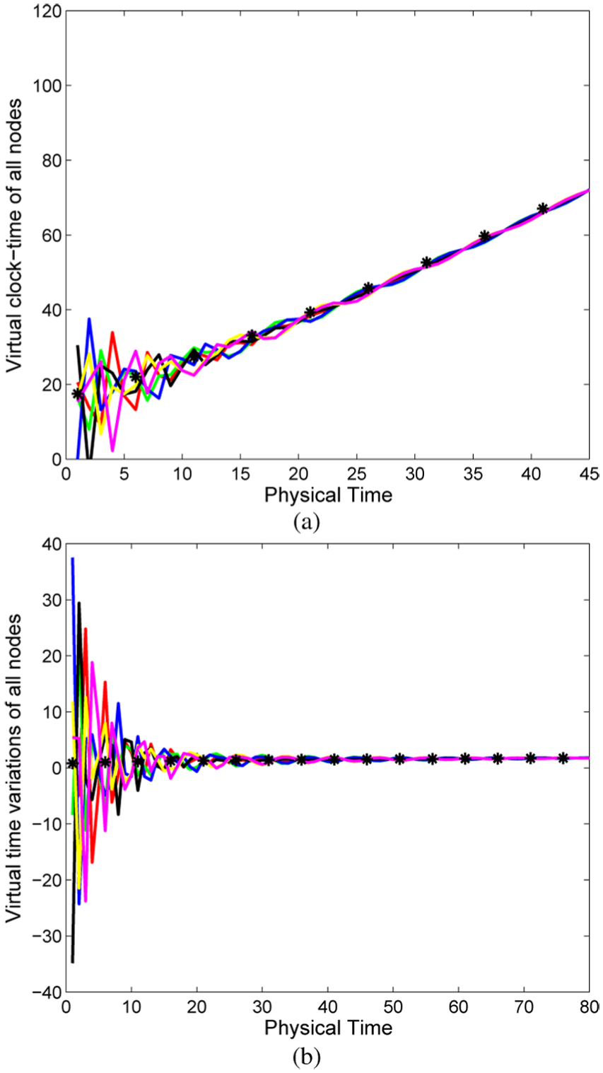
Clock synchronization of the grid with six nodes: (a) changes of virtual time of all local clocks and (b) changes of virtual-time variations of all local clocks.
In this figure, black asterisk markers represent the scatter diagram of the virtual common clock in equation (14). Thus, it can be seen that the synchronization curves can follow the form of equation (14) finally.
Figure 7(b) shows the consensus of virtual-time variations of all local clocks. In this figure, black asterisk markers represent the scatter diagram of the virtual common-time variations as part of equation (14). Then, the two figures show that virtual-time and time variations can almost simultaneously converge to consensus values shown in equation (14). Then according to the definition of
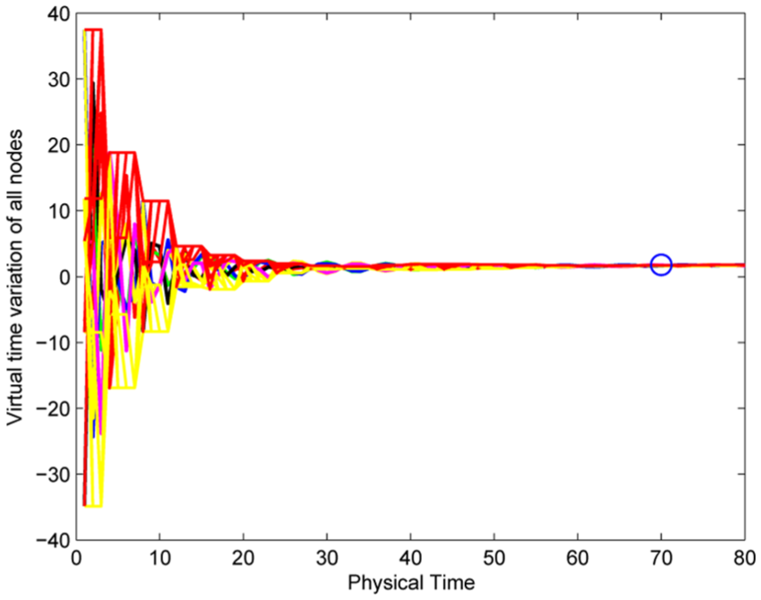
Changes of virtual-time variations with the stopping criterion.
In this figure, the blue circle is the stopping margin picked out by the criterion when
Simulation of changing topologies
With Assumption 2 established, this subsection shows the simulation results when there are changes in the topology.
One more node is added to the net
This simulates certain physical cases. For example, there may be a node off-line or off-power at first. Then, on some physical instant, it is put on line or on power. And when the node is added into the net, other nodes may have been in the synchronization process for a spell. Then, the above situation can be equivalent to the change from Figures 5(a) to 9(a). And the simulation results of this process are shown in Figure 10.

Topology graphs after changes: (a) number of nodes increases and (b) number of nodes decreases.

Synchronization of the net with one more node: (a) synchronization of virtual local time and (b) synchronization of virtual-time variations.
In Figure 10(a), the cyan asterisk denotes the local clock time of node 7 when it is added into the net, and the cyan curve represents the changes of its virtual clock time after it joins with other nodes in running protocols. Similarly, in Figure 10(b), the cyan curve shows the changes of virtual-time variations of node 7. From these figures, we can see that when the new node is added, the previous trend of synchronization is disturbed; however, after node 7 runs the protocols, all nodes can achieve the synchronization eventually.
One node is lost in the net
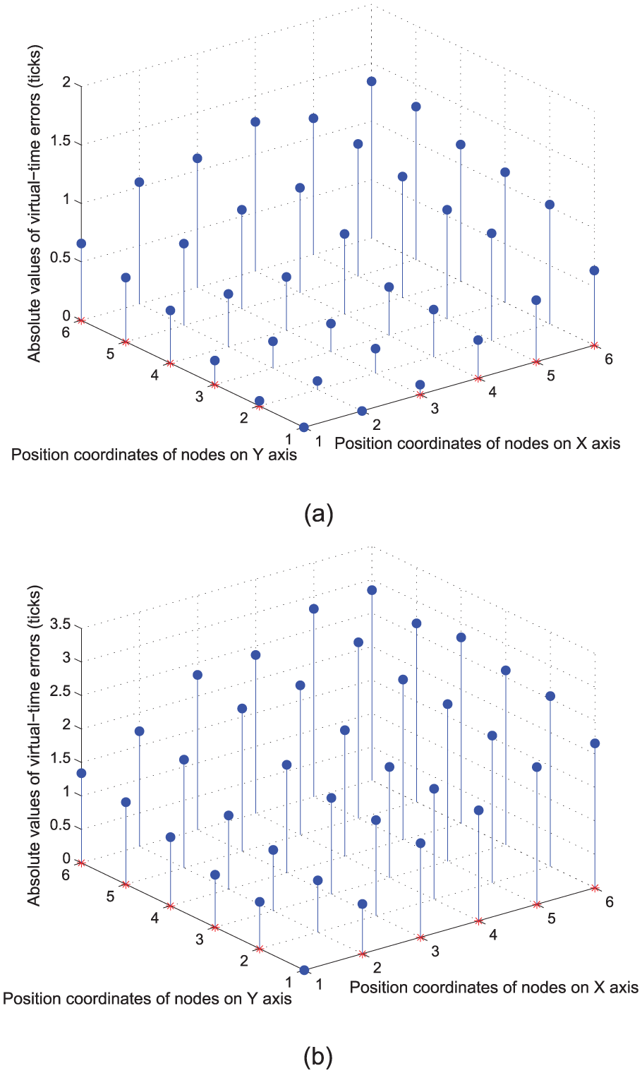
This can simulate the cases that there are packet losses or node failure in the net. These cases can be equivalent to the change from Figure 5(a) to Figure 9(b). Figure 9(b) can represent that node 3 and node 5 cannot acquire the packets from node 4 or node failure happens to node 4. Then, simulation results of this process are shown in Figure 11. In Figure 11(a), the black asterisk denotes the virtual local time of node 4 when it is lost. And it can be seen that after the loss of node 4, the virtual-time errors between other nodes become large for a while, which is specifically shown in Figure 12. Figure 12 is obtained by taking the virtual clock of node 1 as the reference. With the coordinate (1,1) in this figure corresponding to node 1 in Figure 9(b), the X-Y plane can denote the WSN grid in Figure 9(b). Figure 12(a) shows the virtual-time errors on the instant before the loss of node 4, and Figure 12(b) shows the virtual-time errors on the instant after the loss. Then, it can be seen that errors become large between these two instants. However, after remained nodes continue to run protocols, the synchronization can be achieved finally. Similarly, Figure 11(b) shows that the loss of node 4 can influence the errors between virtual-time variations in the process; however, virtual-time variations of all remained nodes can still achieve the synchronization eventually. It is worth mentioning that the black lines in Figure 11 show how virtual-time and time variations of node 4 would change without connection with the net.

Synchronization of the net with one node lost: (a) synchronization of virtual local time and (b) synchronization of virtual-time variations.

Comparison of errors before and after the loss: (a) errors before the loss and (b) errors after the loss.
Simulation of the nets with larger scales
In this section, our protocols are run under the graphs shown in Figure 5(b) and (b), respectively. Then, simulation results can be obtained as shown in Figures 13 and 14 respectively. From these two figures, it can be seen that synchronization of virtual clock time and that of virtual-time variations can still be achieved in the larger nets. So, our protocols can be applied in nets with different scales. Due to the definition of

Clock synchronization of the grid with 36 nodes: (a) changes of virtual time of all local clocks and (b) changes of virtual-time variations of all local clocks.

Clock synchronization of the grid with 800 nodes: (a) changes of virtual time of all local clocks and (b) changes of virtual-time variations of all local clocks.
Comparison of synchronization errors
In this section, protocols in ATS 9 method and those in our method are run under the graph shown in Figure 5(b). Then, Figure 15 is obtained by taking the virtual clock of node 1 as the reference to compare the synchronization errors of these two methods. With coordinates (1,1,0), (2,1,0) and (1,2,0) in this figure corresponding to node 1, 2 and 12 in Figure 5(b) respectively, the X-Y plane can denote the WSN grid in Figure 5(b). From Figure 15, it can be seen that synchronization errors between virtual clocks from both methods are almost proportional to the physical distance between nodes, which is an advantage over TPSN. 6 And comparing Figure 15(a) with Figure 15(b) shows that our method has smaller synchronization errors than the ATS 9 method does under the graph shown in Figure 5(b).
Comparison of synchronization errors: (a) synchronization errors of our method and (b) synchronization errors of the existing method.
Energy consumption analysis
In this section, a recognized energy consumption model 25 for WSNs is utilized to analyze the energy consumption of our protocol. This model contains two main expressions as follows
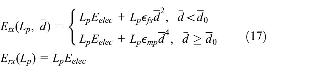
where fs is short for free-space model and mp is short for multi-path model. The physical meanings and typical values of all symbols in the above equations are shown in Table 3.
Symbols and their typical values in the energy consumption model.

Then, with the focus on relatively short-distance transmissions, the transmission distance between nodes in the topology shown in Figure 5(a) is set as

Energy consumption of the grid with six nodes: (a) changes of residual energy due to transmission times and (b) energy consumption with different packet transmission periods.
Conclusion and future work
A new distributed protocol is proposed to achieve synchronization of clock time and that of time variations simultaneously. Its control inputs are robust against noise interference with achievable bounded values. Also, this article provides specific explanations on the virtual clock modeling and communication schemes independent on global physical time. The modified communication scheme enhances robustness against node failure and packet losses and then has a wider application. Finding a stopping margin for the protocols in finite time can conserve more energy. Future work may include researches on optimal choices of parameters to gain better stability and consensus performance. And we plan to conduct more experiments to compare the performance of our method with that of others as certain literature 26 did in the future.
Footnotes
Academic Editor: Olivier Sentieys
Declaration of conflicting interests
The author(s) declared no potential conflicts of interest with respect to the research, authorship, and/or publication of this article.
Funding
The author(s) disclosed receipt of the following financial support for the research, authorship, and/or publication of this article: The work was supported by the National Natural Science Foundation of China (grant no. 61273113) and the Zhejiang Provincial Natural Science Foundation of China (grant no. LR13F030002).