Sage Journals: Discover world-class research

Abstract

A sensor array produces lots of bits of data every sample period, which may cause a heavy burden on the long-distance wireless data transmission, especially in the scenarios of wireless sensor networks. A lossy but error-bounded sensor array data compression algorithm is proposed, in which the major part of the sensor array data are approximated by the Catmull-Rom spline curve and the residual errors are quantized and encoded with Huffman coding. The performance of this algorithm has been evaluated with a real data set from the wireless hydrologic monitoring system deployed in Qinhuangdao Port of China. The results show that the algorithm performs well for the hydrologic sensor array data.

Keywords

Catmull-Rom spline data compression sensor array hydrologic monitoring wireless sensor network

Introduction

Hydrologic data have been employed and making considerable contributions to many applications, such as helping scientists and researchers understand the hydrologic processes and formulate models for hydrologic prediction,^1,2 offering valuable information for mariners to navigate across the ocean,³ and assisting managers at the coastal ports to guide the vessels. There have been far more similar applications. As a result, it is of great significance to collect the hydrologic data to provide essential support to these wide range of situations.

In recent years, wireless sensor networks⁴ offer a superb solution for the long-term, long-distance, and automatic hydrologic data collecting. Wireless sensor networks, which consist of wireless sensor nodes with the capability of sensing, data processing, and wireless communicating, have been extensively applied in various fields.⁵ Wireless sensor networks promise an advantage over the traditional sensing methods in many ways. Besides, they also present a preferable choice in risk-associated applications in the inaccessible regions, such as habitat monitoring, environmental observation, underwater acoustic sensing,^6,7 and hydrologic monitoring.⁸ In fact, hydrologic monitoring systems based on wireless sensor networks have already been developed and deployed in different cases, such as the prototype network of meteorological and hydrological sensors in the Yosemite National Park in the United States,⁹ the flash-flood alerting system with wireless sensor networks for monitoring the environment and tracking natural disasters in the Andean region of Venezuela,¹⁰ and the remote monitoring system for heavy metal ions in water.¹¹ In Qinhuangdao Port of China, a sea route monitoring system has also been deployed, whose major function is to provide underwater flow velocity data to facilitate the safe navigation of the to-and-fro ships.¹²

A sensor array is a group of sensors usually deployed in a certain geometric pattern to sense multiple parameters. Sensor arrays can also be used to record underwater hydrologic conditions at different depths. The wireless hydrologic monitoring system in Qinhuangdao Port of China makes use of sensor arrays to collect underwater flow velocity data to guarantee the safety of the sea routes, as depicted in Figure 1. The sensor array consists of a series of equally spaced sensors. The sensors are installed to a vertical steel cable, and the steel cable is suspended from a buoy. The sensors in the array record flow velocity at different depths and then the data collected will be transferred to the controller on the buoy, which will forward the data further to the shore station through wireless communications, artificial satellites for long-distance communications in particular.

Figure 1.

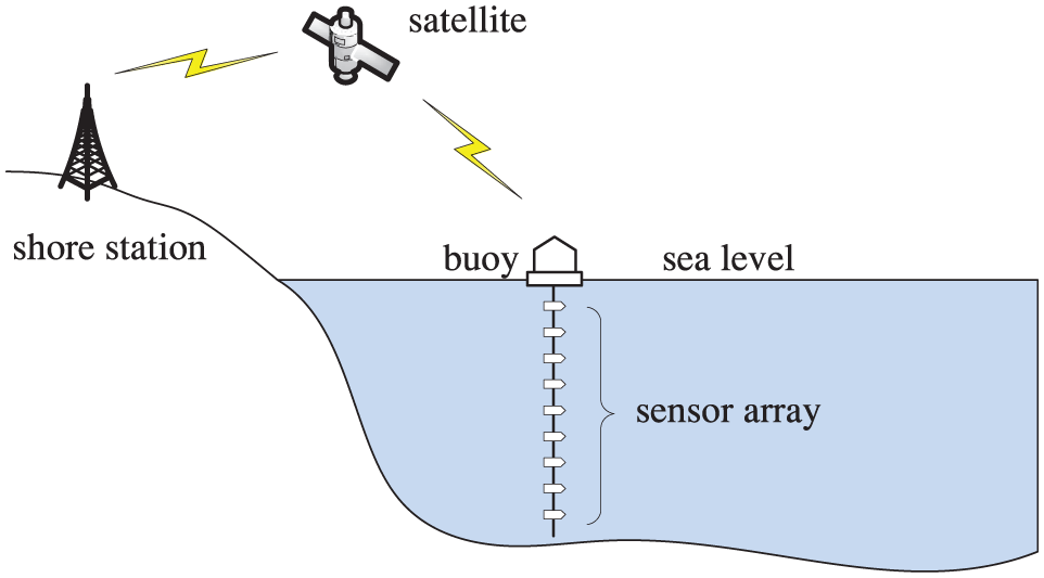
A wireless hydrologic monitoring system.

Data compression is one of the most important schemes to decrease the size of the transmitted data. It leads to a reduction in the required wireless communication, which is the main power consumer in wireless sensor networks.¹³ The sensor array produces lots of bits of data every sample period, which causes a heavy burden on the long-distance wireless data transmission in the hydrologic monitoring systems. All the data should be transferred in a real-time and error-bounded way to support the accurate information publishing for the vessels. Therefore, a compression algorithm for the data of the sensor array is in urgent need to lower the number of bits in data transmissions so as to save transmission cost and also extend the working time of the buoy equipped with batteries.

This article aims to propose an error-bounded low-complexity data compression algorithm for the sensor array in the wireless hydrologic monitoring system. To be specific, our contribution lies mainly in the following aspects. We have introduced a Catmull-Rom Spline curve Approximation algorithm with Error Compensation (CSA/EC) based on the pre-calculated Moore–Penrose pseudoinverse matrix for the sensor array data with a fixed number of equally spaced control points. Note that the algorithm does not depend on the historical data of sensors to ensure the receiver decompresses data in a stateless manner. Then, we have presented a data compression framework, in which the major part of the sensor array data are represented by the Catmull-Rom spline curve and the residual errors are quantized and encoded with Huffman coding. Finally, we have evaluated the performance of our algorithm and other error-bounded compression algorithms with a real data set. The result shows that our algorithm performs well for the hydrologic sensor array data.

The rest of this article is organized as follows: Section “Related works” introduces related works. Section “Preliminary” illustrates the mathematical model. Section “Description of CSA/EC algorithm” proposes our data compression algorithm. Section “Experimental results” presents experimental results. Finally, section “Conclusion” concludes this article.

Related works

Huffman coding¹⁴ is an entropy variable-length encoding algorithm used for lossless data compression. Huffman coding adopts a specific method for choosing the representation for each symbol based on the frequency of occurrence of the symbol. A symbol that has a very high probability of occurrence generates a code with very few bits, while a symbol with a low probability generates a code with a larger number of bits. Codes are stored in a codebook to encode and decode. Huffman coding is one of the most efficient compression methods of individual source symbols when the actual symbol frequencies agree with those used to create the code. However, if the data of all sensors in the sensor array are regarded as a vector symbol, the codebook will be too large to construct or store in the buoy controllers; if regarded as a collection of individual scalar symbols, the data correlation of adjacent sensors is totally ignored. Thus, Huffman coding is not an ideal approach for data compression of the hydrologic sensor array.

Lossy compression methods ought to be taken into consideration as regards to the data compression of the hydrologic sensor array since the data here are not required to be exactly accurate. Lossy compression methods usually produce good compression ratio in general, for instance, JPEG (Joint Photographic Experts Group),¹⁵ discrete cosine transform (DCT),¹⁶ and vector quantization (VQ).¹⁷ If the sensor array data are treated as a multi-dimensional vector, some dimensionality reduction methods may be able to apply in our situation. Principal Component with Vector Quantization (PCVQ)¹² compression method has been proposed for the hydrologic data. However, although the average data error decreases with an increase in the size of the codebook, the maximum error is not bounded. Since the maximum errors of these lossy compression methods are not guaranteed to be bounded, it may lead to inaccurate results in the worst cases.

As a basic lossy but error-bounded compression method, quantization is the procedure for reducing the number of bits needed to store an integer value by reducing the precision of the integer. Quantization is usually for scalar values. An adaptive piecewise constant approximation (APCA) algorithm¹⁸ was designed to apply to time-series data set but it is also suitable for the space-series data, such as the data from sensors at different depths in our case. APCA algorithm ignores certain fluctuation in the data. A segment grows until deviation exceeds the error threshold and then the segment can be represented by a single value. The maximum error by quantization and APCA algorithms can be bounded to a certain constant, which will play a pivotal role in some specific data analyses.

We summarize all the compression algorithms mentioned above in Table 1.

Table 1.

The comparison of mentioned compression methods.

Compression algorithms	Lossless/lossy	Error-bounded
Huffman	Lossless
JPEG	Lossy	No
DCT	Lossy	No
VQ	Lossy	No
PCVQ	Lossy	No
Quantization	Lossy	Yes
APCA	Lossy	Yes

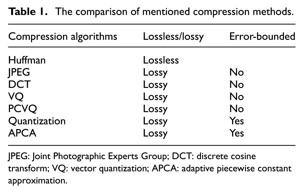
JPEG: Joint Photographic Experts Group; DCT: discrete cosine transform; VQ: vector quantization; APCA: adaptive piecewise constant approximation.

In addition, there are kinds of curves that are represented with just a small number of parameters, that is, control points for lossy data compression. Data can be regenerated using control points through interpolation at the receiver.^19–21 Utilize spline interpolation to reconstruct the physical world. Quadratic Bézier curve and Catmull-Rom spline were introduced to compress video data.^22,23 Reducing the data errors caused by the compression,²⁰ acquires control points through adjusting the sensing frequency and²³ selects control points according to the maximum allowed error. The original versions of the related data compression methods with splines are usually not error-bounded, or not for real-time applications. But they laid a foundation to construct the enhanced algorithm introduced in this article.

Preliminary

Catmull-Rom spline

Catmull-Rom spline²⁴ is a family of the $C^{1}$ continuous cubic interpolating splines. Let $p_{1}, p_{2}, \dots, p_{M}$ represent the control points. Each control point $p_{i}$ represents a two-dimensional vector $(p_{i}^{x}, p_{i}^{y})$ , where $1 \leq i \leq M$ . Tangent at each point $p_{i}$ is calculated using the previous and the next point on the curve, that is, ${p^{'}}_{i} = τ (p_{i + 1} - p_{i - 1})$ . Parameter $τ$ affects how sharply the curve bends at control points and is often set to 1/2.

The $i th$ segment of the curve between $p_{i}$ and $p_{i + 1}$ is determined by four control points, that is, $p_{i - 1}, p_{i}, p_{i + 1}$ , and $p_{i + 2}$ , as depicted in Figure 2.

Figure 2.

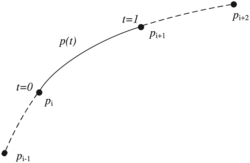
A segment of Catmull-Rom spline.

Now that the segment of the Catmull-Rom spline is cubic, and the $i th$ segment can be expressed by a polynomial form like

p (t) = c_{0} + c_{1} t + c_{2} t^{2} + c_{3} t^{3}

(1)

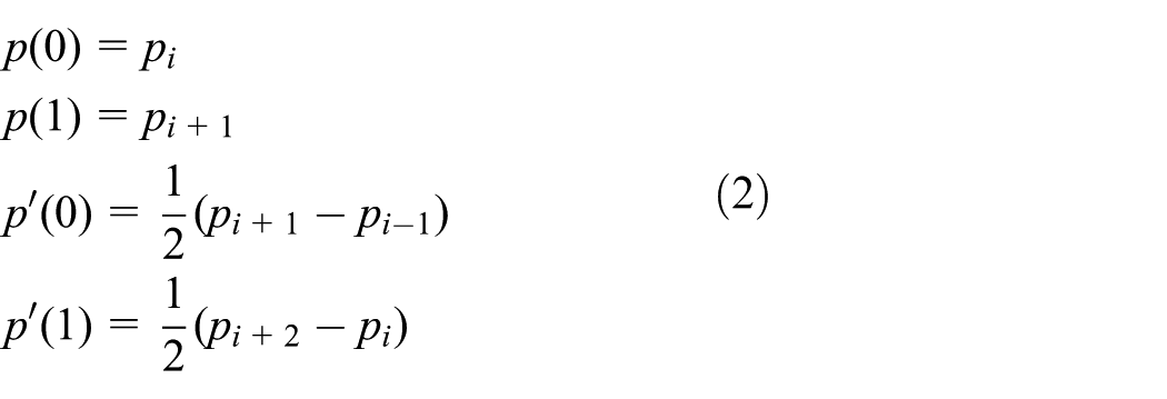
Equation (1) is restricted by

\begin{matrix} p (0) = p_{i} \\ p (1) = p_{i + 1} \\ p' (0) = \frac{1}{2} (p_{i + 1} - p_{i - 1}) \\ p' (1) = \frac{1}{2} (p_{i + 2} - p_{i}) \end{matrix}

(2)

By combining equations (1) and (2), we always have

p (t) = \frac{1}{2} {[\begin{matrix} - t + 2 t^{2} - t^{3} \\ 2 - 5 t^{2} + 3 t^{3} \\ t + 4 t^{2} - 3 t^{3} \\ - t^{2} + t^{3} \end{matrix}]}^{T} \cdot [\begin{matrix} p_{i - 1} \\ p_{i} \\ p_{i + 1} \\ p_{i + 2} \end{matrix}]

(3)

where $t \in [0, 1]$ is the parameter of interpolation.

Representing sensor array data

Consider that there are N sensors $S_{1}, S_{2}, \dots, S_{N}$ in the sensor array. These sensors are deployed at depths ranging from $x_{1}$ to $x_{N}$ with an interval of $(x_{N} - x_{1}) / (N - 1)$ . Without loss of generality, we suppose that the interval of two adjacent sensors is a distance unit and the origin of the vertical coordinate is appropriately selected so that $x_{i} = i$ for $1 \leq i \leq N$ .

At a given moment, let the value of sensor $S_{i}$ be denoted as $y_{i}$ . To represent the data of the sensor array, we define an $N \times 1$ matrix $Y$ as follows

Y = {[y_{1}, y_{2}, \dots, y_{N}]}^{T}

(4)

Now, let us approximately represent data $Y$ with a small number of parameters based on the Catmull-Rom spline curve, as depicted in Figure 3.

Figure 3.

Representing sensor array data with the Catmull-Rom spline curve.

Let M denote the number of control points of the Catmull-Rom spline and $p_{i}$ denote the $i th$ control point. Let control points be equally spaced along the x-axis. That is to say

p_{i}^{x} = 1 + \frac{(i - 1) (N - 1)}{M - 1}

(5)

Obviously, there are $M - 1$ segments in the Catmull-Rom spline curve. The x coordinate of the point in the $i th$ segment satisfies $p_{i}^{x} \leq x \leq p_{i + 1}^{x}$ . Now that the Catmull-Rom spline is continuous, there is no difference whether the boundaries of the segments belong to the left segment or the right one.

Let $B$ denote an $M \times 1$ matrix of ${p_{i}^{y}}$

\begin{matrix} B = {[b_{1}, b_{2}, \dots, b_{M}]}^{T} \\ = {[p_{1}^{y}, p_{2}^{y}, \dots, p_{M}^{y}]}^{T} \end{matrix}

(6)

In other words, ${b_{i}}$ is a collection of the tunable parameters of the Catmull-Rom spline.

In addition, we place two additional virtual control points for the first and the last segments of the spline, as illustrated in Figure 4.

Figure 4.

Additional virtual control points.

The virtual control points satisfy

\begin{matrix} p_{0} = (1 - \frac{N - 1}{M - 1}, b_{1}) \\ p_{M + 1} = (N + \frac{N - 1}{M - 1}, b_{M}) \end{matrix}

(7)

If the $j th$ sensor belongs to the $k_{j} th$ segment, then we have

k_{j} = ⌈ \frac{(j - 1) (M - 1)}{N - 1} ⌉

(8)

where ⌈·⌉ is used to denote the ceil function

⌈ x ⌉ = {\begin{matrix} x x \in Z \\ smallest integer that is greater than x otherwise \end{matrix}

Now, we calculate the reconstructed data by the tunable parameters ${b_{i}}$ . Since sensor $S_{j}$ belongs to the $k_{j} th$ segment of the spline, the parameter of interpolation $t_{j}$ satisfies

\begin{matrix} t_{j} = \frac{x_{j} - p_{k_{j}}^{x}}{p_{k_{j + 1}}^{x} - p_{k_{j}}^{x}} \\ = \frac{j - p_{k_{j}}^{x}}{(N - 1) / (M - 1)} \end{matrix}

(9)

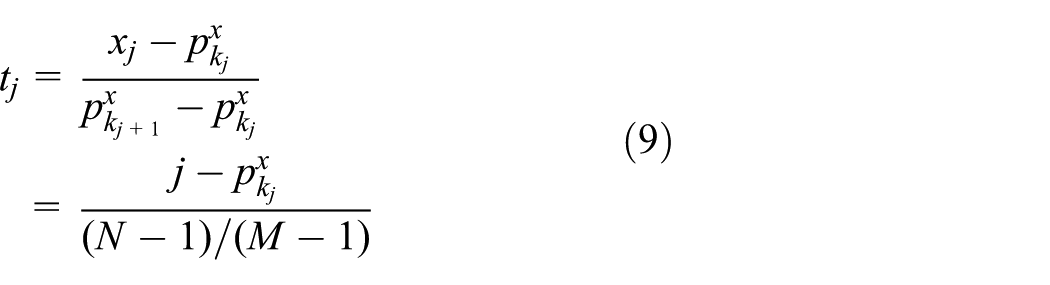
From equation (3), the interpolated value ${\hat{y}}_{j}$ at $x_{j}$ is given by

{\hat{y}}_{j} = \frac{1}{2} {[\begin{matrix} - t_{j} + 2 t_{j}^{2} - t_{j}^{3} \\ 2 - 5 t_{j}^{2} + 3 t_{j}^{3} \\ t_{j} + 4 t_{j}^{2} - 3 t_{j}^{3} \\ - t_{j}^{2} + t_{j}^{3} \end{matrix}]}^{T} \cdot [\begin{matrix} b_{k_{j - 1}} \\ b_{k_{j}} \\ b_{k_{j + 1}} \\ b_{k_{j + 2}} \end{matrix}]

(10)

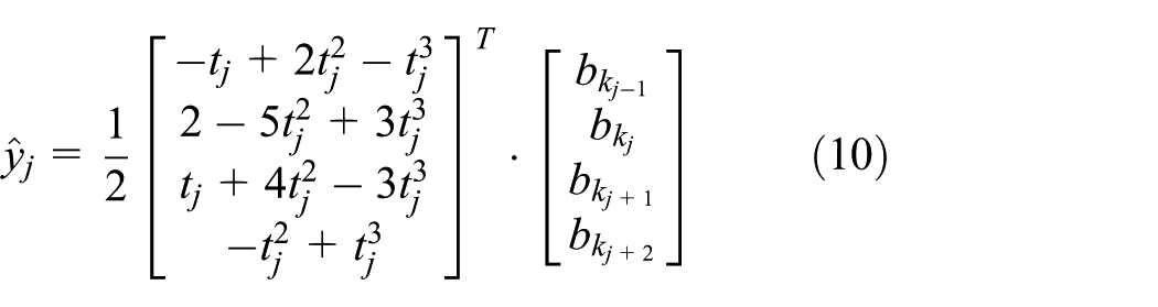
Now, define $a_{j, i}$ as

a_{j, i} = {\begin{matrix} \frac{- t_{j} + 2 t_{j}^{2} - t_{j}^{3}}{2} & i = k_{j - 1} \\ \frac{2 - 5 t_{j}^{2} + 3 t_{j}^{3}}{2} & i = k_{j} \\ \frac{t_{j} + 4 t_{j}^{2} - 3 t_{j}^{3}}{2} & i = k_{j + 1} \\ \frac{- t_{j}^{2} + t_{j}^{3}}{2} & i = k_{j + 2} \\ 0 & otherwise \end{matrix}

(11)

Thus, equation (10) can be written as

{\hat{y}}_{j} = {[\begin{matrix} a_{j, 1} \\ ⋮ \\ a_{j, i - 1} \\ a_{j, i} \\ a_{j, i + 1} \\ a_{j, i + 2} \\ ⋮ \\ a_{j, M} \end{matrix}]}^{T} \cdot [\begin{matrix} b_{1} \\ ⋮ \\ b_{i - 1} \\ b_{i} \\ b_{i + 1} \\ b_{i + 2} \\ ⋮ \\ b_{M} \end{matrix}]

(12)

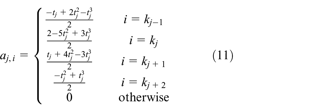
Furthermore, equation (12) leads to

\hat{Y} = AB

(13)

where

\hat{Y} = {[{\hat{y}}_{1}, {\hat{y}}_{2}, \dots, {\hat{y}}_{N}]}^{T}

and

A = {[a_{j, i}]}_{N \times M}

Hence, we solve the optimal parameters

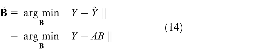
\begin{matrix} \tilde{B} = \underset{B}{\arg \min} ∥ Y - \hat{Y} ∥ \\ = \underset{B}{\arg \min} ∥ Y - AB ∥ \end{matrix}

(14)

where ∥·∥ is used to denote the matrix norm

∥ X_{n \times m} ∥ = \sum_{i = 1}^{n} {(\sum_{j = 1}^{m} | x_{ij} |^{2})}^{1 / 2}

Let $A^{+}$ denote the Moore–Penrose pseudoinverse of the matrix $A$ . Accordingly, the optimal $\tilde{B}$ is given by

\tilde{B} = A^{+} Y

(15)

Note that $A$ is independent of $Y$ . In this case, $A^{+}$ can be stored beforehand for future calculation.

Description of CSA/EC algorithm

A novel sensor array compression algorithm is introduced in this article, abbreviated to CSA/EC. The framework of the algorithm is illustrated in Figure 5.

Figure 5.

Framework of the data compression algorithm based on Catmull-Rom spline approximation.

There are two parts in Figure 5. The left part depicts the procedures in the transmitter and the right part depicts those in the receiver. The sensor number N and the control point number M are given constants.

In the transmitter, the sensor array generates data $Y$ each sample period. The optimal spline parameter $\tilde{B}$ is calculated according to equation (15). Since $A$ only depends on N and M, $A$ and its Moore–Penrose pseudoinverse $A^{+}$ are calculated before the procedure of data compression.

The approximate value of the sensor array data by the spline parameter $\tilde{B}$ is given by

\hat{Y} = A \tilde{B}

(16)

Note that $\tilde{B}$ is quantized for transmission. The approximate value captures the major part of the real value, but the residual error should not be ignored if the number of the control points is not enough. The error between the real value and the approximate value is

Δ = Y - \hat{Y}

(17)

Quantization is applied to $Δ$ . The quantized result is encoded to $E$ with Huffman coding, and the codebook is pre-calculated with historical data. The transmitter sends both $\tilde{B}$ and $E$ to the receiver.

The receiver reconstructs the approximate value $\hat{Y}$ according to equation (16) and decodes $E$ to quantized error $Δ^{'}$ . The final result in the data decompression is given as

Y^{'} = \hat{Y} + Δ^{'}

(18)

CSA/EC is depicted in Algorithm 1. When a group of data are produced by the sensor array, it will be compressed and the compressed data can be transmitted to the satellite or other wireless channels.

Algorithm 1 CSA/EC compression algorithm.
Require: The data produced by sensor array, $Y$ ; The matrix of interpolated coefficients calculated according to the number of sensors N and the number of control points M, $A$ ; The Moore-Penrose pseudoinverse of $A$ , $A^{+}$ ;
Ensure: The $M \times 1$ matrix of optimal spline parameters, $\tilde{B}$ ; The error between the real value and the approximate value encoded with Huffman coding, $E$ .
1: Calculate the optimal spline parameter $\tilde{B}$ according to equation (15);
2: Generate the approximate value $\hat{Y}$ according to equation (16);
3: Calculate the error $Δ$ between $Y$ and $\hat{Y}$ according to equation (17);
4: Quantize and encode $Δ$ to $E$ with Huffman coding;
5: return $\tilde{B}$ and $E$ .

In our compression algorithm, the data errors are only derived from the quantization of the residual error. Thus, the maximum error is bounded by the quantization step size. It is worthy to pay attention to the fact that the computational delay of CSA/EC is constant. It is a low-complexity compression algorithm and is easy to be implemented in the embedded controllers.

The decompression procedure of CSA/EC is depicted in Algorithm 2. Note that the decompression algorithm is also of low complexity.

Algorithm 2 CSA/EC decompression algorithm.
Require: The $M \times 1$ matrix of optimal spline parameters, $\tilde{B}$ ; The error between the real value and the approximate value encoded with Huffman coding, $E$ .
Ensure: The reconstructed data $Y^{'}$ ;
1: Obtain $Δ$ from $E$ with Huffman decoding;
2: Generate the approximate value $\hat{Y}$ according to equation (16);
3: Calculate the reconstructed data $Y^{'}$ according to equation (18);
4: return $Y^{'}$ .

Experimental results

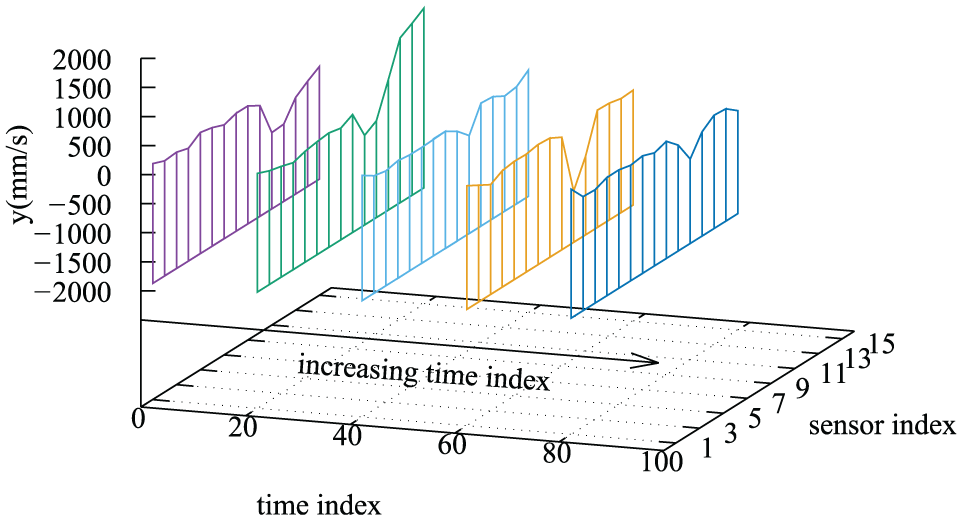
We conduct experiments to evaluate the effectiveness of the proposed algorithm based on a practical data set collected by a sensor array in Qinhuangdao Port during the period from September 2012 to December 2012. The data set is demonstrated in Figure 6.

Figure 6.

Visualization of the data used in the experiments.

There are $N = 15$ sensors in the sensor array. At a given instant, the sensing value of each sensor is an integer ranging from −4096 to 4095, that is, 13 bits, which expresses the flow velocity of the corresponding depth in millimeter per second (mm/s). The sampling period is 10 min. Thus, it means a 15-dimensional vector is produced every 10 min. The amount of the total data generated at one sample moment is $13 \times 15 = 195 bits$ . A representative segment of the practical data is shown in Figure 7.

Figure 7.

Time series of sensor values from 12:06:54 p.m. on 15 December 2012 to 05:06:54 a.m. on 16 December 2012.

Each subgraph in Figure 7 depicts a time series which contains the sensing values of 100 sample periods generated by a given sensor. For simplicity of presentation, we only list the subgraphs corresponding to the sensors labeled No. 1, No. 5, No. 10, and No. 15. Here, the sensors are indexed from top to bottom. The beginning time of the segment is 12:06:54 p.m. on 15 December 2012 and the ending time is 05:06:54 a.m. on 16 December 2012.

All the algorithms mentioned in this section are implemented with MATLAB. The following experiments were conducted on a desktop computer with 8 GB memory and an Intel i7 processor (2.5 GHz). But it is worth noting that the proposed CSA/EC algorithm is not time consuming and we can easily implement it on an embedded controller.

Figure 8 shows the result of interpolating sensor array data with the Catmull-Rom spline at one sample moment. Comparing the original data with the interpolated data with different numbers of control points, we conclude that the interpolated data on the spline curves reflect the major fluctuation of the original data. The increase in the number of control points often, but not always, leads to the decrease in the residual errors. Theoretically, with the same number of control points as the sensors in the array, we will obtain a perfect Catmull-Rom spline which is identical to the original data but without any data reduction.

Figure 8.

Original data and interpolated data.

As previously mentioned, the interpolated values by the Catmull-Rom spline only reflect the major part of the sensor array data. However, the residual errors are concentrated to zero, as depicted in Figure 9.

Figure 9.

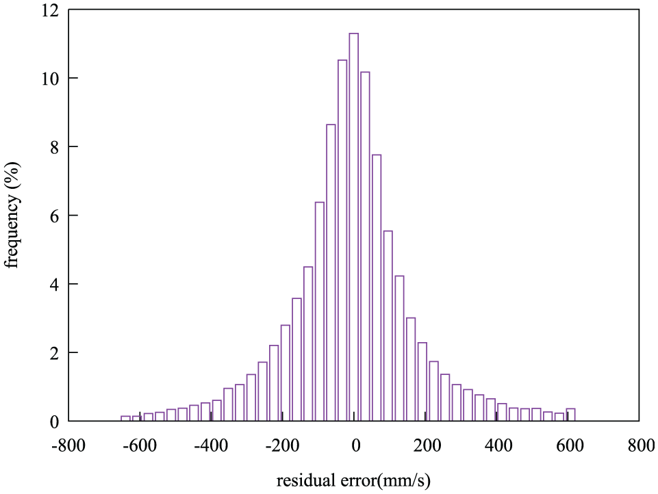
The distribution of the residual errors.

As the values of original sensor data are sparsely distributed from −4096 to 4095, it is observed that the residual errors range approximately from −600 to 600, and actually 70% of them are limited from −128 to 128. Thus, for the residual errors, Huffman coding is efficient and the size of the codebook is small.

Now, we compare our algorithm with other error-bounded lossy data compression algorithms. The goal of our algorithm is to markedly reduce the transmitted data. To measure the data reduction performance of compression algorithms, we define compression ratio as

r_{c} = (1 - \frac{S_{c}}{S_{o}}) \times 100 %

(19)

where $S_{c}$ is the compressed size, that is, the data size after running compression algorithms. $S_{o}$ is the original data size. Both are measured with the number of bits. Note that the original data generated by the sensor array are 195 bits in a sample period.

All the packet formats to store the compressed data of different algorithms are shown in Figure 10.

Figure 10.

Packet format to represent the compressed data.

Quantization is a basic lossy compression method. The values of each sensor are quantized and transferred one by one in a packet. If the maximum error bound $E_{\max}$ is 8, then the quantization step size is 16 and the number of bits for the data of each sensor is 9. Thus, the compressed data size with quantization method for $E_{\max} = 8$ , denoted by Q-8, is fixed and equal to $9 \times N = 135 bits$ . Similarly, the compressed data size with quantization method for $E_{\max} = 16$ , denoted by Q-16, is 120 bits.

APCA is another error-bounded lossy data compression method to be compared. In APCA, the compressed data are represented as $(x, y)$ coordinate pairs, that is, the sensor indexes and sensor values, with each pair for one segment of constant. The number of bits for sensor index is 4 and that for sensor value is 13. The number of pairs should also be transferred with 4 bits. However, since the sensor index of the first pair is always 1, it can be omitted to save 4 bits. Let APCA-8 denote APCA method with the maximum error bound $E_{\max} = 8$ and so forth.

ACSA (Adaptive Catmull-Rom Spline curve Approximation) is a simple error-bounded lossy data compression with spline function inspired by Chakrabarti et al.,¹⁸ Reise et al.,¹⁹ and Li et al.²⁰ In the algorithm of ACSA, the control points are selected as few as possible constrained by the maximum error bound. Initially, it selects the minimal number of control points to construct the spline. If the residual error of a point is beyond the maximum error bound, the point will be added as a control point. The aforementioned procedure is executed iteratively until all the residual errors are smaller than the maximum error bound. The compressed data can also be represented as $(x, y)$ coordinate pairs, that is, the control point indexes and values. The number of bits for control point index is 4 and that for value is 13. The number of pairs should also be transferred with 4 bits. Similarly, since the index of the first pair is always 1, it can be omitted to save 4 bits. Let ACSA-8 denote ACSA method with the maximum error bound $E_{\max} = 8$ and so forth.

In our algorithm, that is, CSA/EC, the compressed data consist of two parts. The former is a fixed-length record to represent the Catmull-Rom spline parameters. The latter is a variable-length record to represent the residual errors. In our experiments, the number of control points of the Catmull-Rom spline is set to 4. The quantization step size of $\tilde{B}$ is 64. Thus, the size of the former part is 28 bits. The quantization step size of the residual errors depends on the maximum error bound. Note that the values $e_{1}, e_{2}, \dots, e_{N}$ are quantized residual errors encoded with Huffman coding. Analogically, CSA/EC-8 denotes the CSA/EC algorithm with the maximum error bound $E_{\max} = 8$ and so forth.

Figures 11 and 12 show the sizes of the compressed data by different methods in detail for 100 samples randomly chosen from the real data set with the maximum error bounds set to 8 and 32, respectively. The performance of APCA and ACSA has similar results because both of them dynamically select the control points. CSA/EC has a relatively small size of compressed data compared to other algorithms with the maximum error bound $E_{\max} = 8$ . Compressed data size falls significantly with the maximum error bound $E_{\max} = 32$ . CSA/EC also exhibits a stable performance compared with ACSA and APCA.

Figure 11.

The compressed data sizes of 100 sample periods ( $E_{\max} = 8$ ).

Figure 12.

The compressed data sizes of 100 sample periods ( $E_{\max} = 32$ ).

Using the complete data set from September 2012 to December 2012, we obtain a more convincing results. Figure 13 presents comparison of average compression ratios of CSA/EC and other lossy error-bounded algorithms with different maximum error bounds. All these algorithms achieve higher compression ratios with an increase in the set maximum error bound. CSA/EC has an outstanding advantage over other algorithms. The details of CSA/EC and other algorithms in terms of compressed data size and compression ratio with different maximum error bounds on our data set are listed in Table 2.

Figure 13.

The compression ratios of different maximum error bounds.

Table 2.

The comparison of CSA/EC and other algorithms.

Maximum error bound	Algorithm	Compressed size (bit)	Compression ratio (%)
0	Original data	195	0.0
8	Q-8	135	30.7
8	APCA-8	238.2	−22.1
8	ACSA-8	241.2	−23.6
8	CSA/EC-8	114.4	41.3
16	Q-16	120	38.5
16	APCA-16	221.5	−13.6
16	ACSA-16	226.3	−16.1
16	CSA/EC-16	95.2	51.2
32	Q-32	105	46.1
32	APCA-32	192.6	0.0
32	ACSA-32	203.7	−0.1
32	CSA/EC-32	77.4	60.3
64	Q-64	90	53.8
64	APCA-64	148.8	23.7
64	ACSA-64	162.5	16.7
64	CSA/EC-64	59.7	69.4

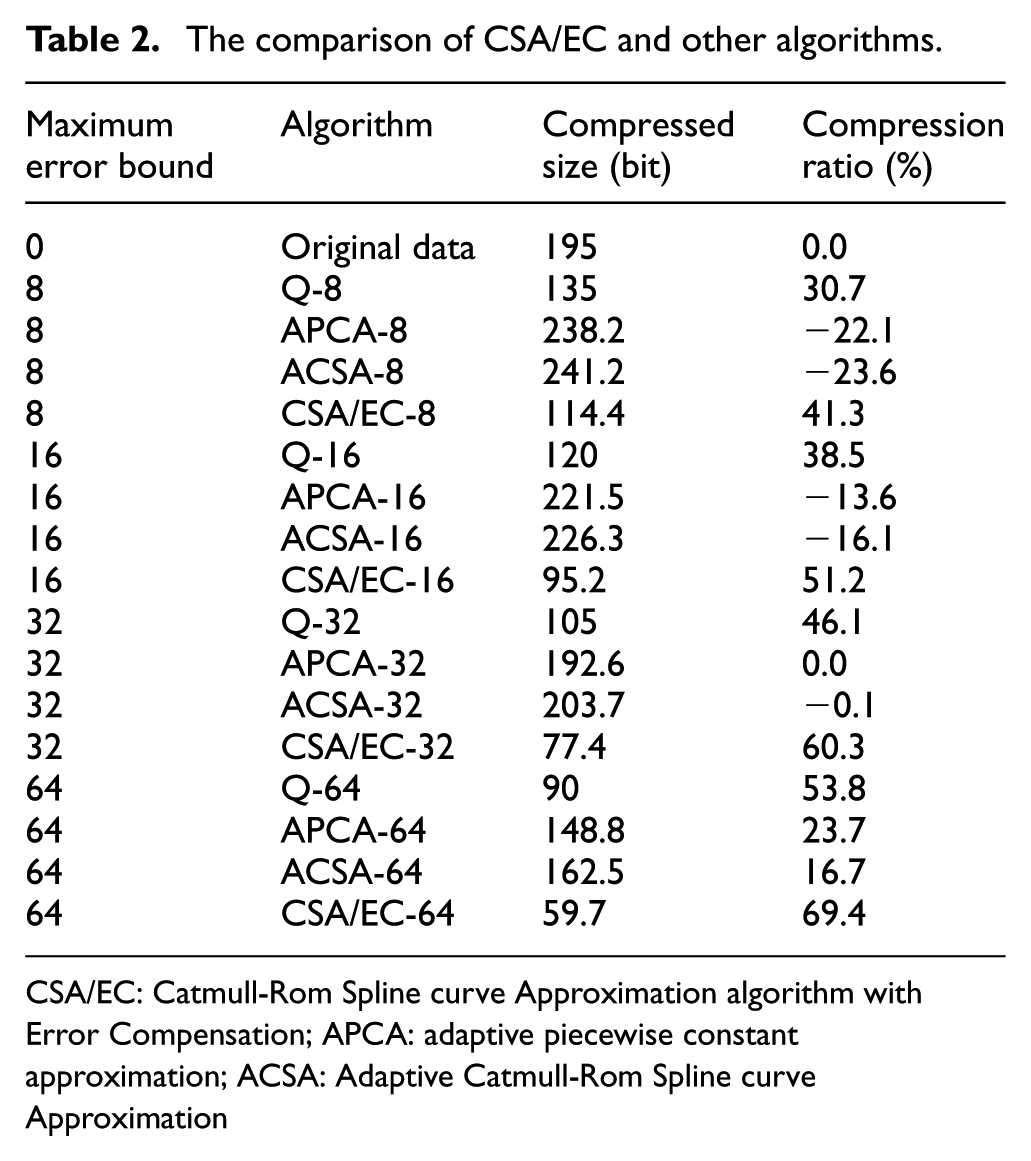
CSA/EC: Catmull-Rom Spline curve Approximation algorithm with Error Compensation; APCA: adaptive piecewise constant approximation; ACSA: Adaptive Catmull-Rom Spline curve Approximation

The experimental results indicate that the CSA/EC algorithm is obviously superior to other algorithms. The sensor array data are saved 41.3% of the original size when $E_{\max} = 8$ , or 69.4% of that when $E_{\max} = 64$ , by our CSA/EC algorithm. In both cases, the compression ratio of our algorithm is at least 10% better than that of the quantization method and almost 60% better than that of the APCA and ACSA methods.

Conclusion

Sensor arrays in a certain geometric pattern are often used to record conditions. Data compression is of great importance to data collecting with wireless sensor networks since the sensor array produces lots of bits of data every sample period. We propose an error-bounded lossy sensor array data compression algorithm, in which the major part of the sensor array data are represented by the Catmull-Rom spline curve and the residual errors are quantized and encoded with Huffman coding. The algorithm is also of low complexity and a stateless, which can be easily implemented in the embedded micro-controller in a wireless sensor network.

We have evaluated the performance of our algorithm and other error-bounded compression algorithms with a real data set from the wireless hydrologic monitoring system deployed in Qinhuangdao Port of China. The result shows that our algorithm performs well for the hydrologic sensor array data. Furthermore, our algorithm is not limited to underwater hydrologic monitoring. It is suitable for any sensor array in a linear geometric pattern as long as the major part of the data are possibly represented by a spline and the residual errors are convergent enough.

Footnotes

Academic Editor: Maio Jin

Declaration of conflicting interests

The author(s) declared no potential conflicts of interest with respect to the research, authorship, and/or publication of this article.

Funding

The author(s) disclosed receipt of the following financial support for the research, authorship, and/or publication of this article: This work was supported by National Natural Science Foundation of China (61370191), MoE (Ministry of Education) and China Mobile Limited Joint Foundation (No. MCM20160103), the Fundamental Research Funds for the Central Universities of China (FRF-BR-15-081a), and the Foundation of Beijing Engineering and Technology Center for Convergence Networks and Ubiquitous Services.

References

Clark

Fan

Lawrence

. Improving the representation of hydrologic processes in earth system models. Water Resour Res 2015; 51(8): 5929–5956.

Lettenmaier

DP.

Hydrologic prediction over the conterminous United States using the national multi-model ensemble. J Hydrometeorol 2014; 15(4): 1457–1472.

Park

E-navigation-supporting data management system for variant S-100-based data. Multimed Tool Appl 2015; 74(16): 6573–6588.

Akyildiz

Sankarasubramaniam

. Wireless sensor networks: a survey. Comput Netw 2002; 38(4): 393–422.

Yick

Mukherjee

Ghosal

Wireless sensor network survey. Comput Netw 2008; 52(12): 2292–2330.

Han

Zhang

Liu

. MANCL: a multi-anchor nodes collaborative localization algorithm for underwater acoustic sensor networks. Wireless Comm Mobile Comput 2014; 16: 682–702.

Cho

Chen

Shih

. Survey on underwater delay/disruption tolerant wireless sensor network routing. IET Wirel Sens Syst 2014; 4(3): 112–121.

A survey of sensor network applications. IEEE Commun Mag 2002; 40(8): 102–114.

Lundquist

Cayan

Dettinger

MD.

Meteorology and hydrology in Yosemite national park: a sensor network application. In: Zhao

Guibas

(eds) Information processing in sensor networks. Berlin: Springer, 2003, pp.518–528.

10.

Castillo-Effer

Quintela

Moreno

. Wireless sensor networks for flash-flood alerting. In: Proceedings of the fifth IEEE international caracas conference on devices, circuits and systems (vol. 1), Punta Cana, Dominican Republic, 3–5 November 2004, pp.142–146. New York: IEEE.

11.

Dexia

Wenjun

. Design of remote monitoring system for heavy metal ions in water. In: Proceedings of the 26th Chinese control and decision conference (2014 CCDC), Changsha, China, 31 May–2 June 2014, pp.5070–5073. New York: IEEE.

12.

Zhang

Huangfu

. Sea route monitoring system using wireless sensor network based on the data compression algorithm. China Commun 2014; 11(13): 179–186.

13.

Srisooksai

Keamarungsi

Lamsrichan

. Practical data compression in wireless sensor networks: a survey. J Netw Comput Appl 2012; 35(1): 37–59.

14.

Huffman

DA.

A method for the construction of minimum-redundancy codes. Proc IRE 1952; 40(9): 1098–1101.

15.

Higgins

Mc Ginley

Glavin

. Low power compression of EEG signals using JPEG2000. In: Proceedings of the 4th international conference on pervasive computing technologies for healthcare, Munich, 22–25 March 2010, pp.1–4. New York: IEEE.

16.

Bendifallah

Benzid

Boulemden

Improved ECG compression method using discrete cosine transform. Electron Lett 2011; 47(2): 87–89.

17.

Chen

. Improved vector quantization scheme for grayscale image compression. Opto-Electron Rev 2012; 20(2): 187–193.

18.

Chakrabarti

Keogh

Mehrotra

. Locally adaptive dimensionality reduction for indexing large time series databases. ACM T Database Syst 2002; 27(2): 188–228.

19.

Reise

Matz

Grochenig

Distributed field reconstruction in wireless sensor networks based on hybrid shift-invariant spaces. IEEE T Signal Process 2012; 60(10): 5426–5439.

20.

Cheng

Gao

. Approximate physical world reconstruction algorithms in sensor networks. IEEE T Parall Distr 2014; 25(12): 3099–3110.

21.

Tseng

Cho

Chou

. Efficient power conservation mechanism in spline function defined WSN terrain. IEEE Sens J 2014; 14(3): 853–864.

22.

Khan

Ohno

. Compression of temporal video data by Catmull-Rom spline and quadratic Bézier curve fitting. In: Proceedings of the international conference in Central Europe on computer graphics, visualization and computer vision, Plzen - Bory, 4–7 February 2008.

23.