Sage Journals: Discover world-class research

Abstract

Growth of the traffic flow and traffic accident has raised more and more demands on wireless communication and positioning technologies that can provide new services such as vehicle collision warning and traffic management. Currently, the global navigation satellite system such as global positioning system and BeiDou satellite positioning system is widely used in vehicles and is fairly accurate in flat open areas. However, the global navigation satellite system can only work in line of sight environment, and it fails to operate in non-line of sight tunnels or downtown areas where blockage of satellite signals is frequent. Because of the shortages of global navigation satellite system, the wireless ranging or positioning system using the short preamble of IEEE 802.11p is provided. Typically, accurate time of arrival estimation is very important for positioning estimation. In order to improve the precision of the time of arrival estimation, a correlation-sum-deviation method for ranging using the IEEE 802.11p short preamble is proposed. Simulation results are presented which show that in both the additive white Gaussian noise channel and the international telecommunications union multipath channel for vehicular environments, the proposed method provides better precision and is less complex than other techniques, particularly when the signal-to-noise ratio is low.

Keywords

Vehicle positioning ranging time of arrival estimation IEEE 802.11p cross-correlation

Introduction

The report by the World Health Organization (WHO)¹ indicates that worldwide the total number of road traffic deaths remains unacceptably high at 1.24 million per year, road traffic injuries are the eighth leading cause of death globally, and the leading cause of death for young people aged 15–29 years. Current trends suggest that by 2030, road traffic deaths will become the fifth leading cause of death unless urgent action is taken.² The most promising actions are the development of cooperative collision avoidance (CCA) and emergency warning message (EWM) systems in vehicular ad hoc networks (VANETs)³ where each vehicle can predict potential hazards and can take proper steps to avoid collision by sharing information such as location, speed, acceleration, and so on. The major characteristic of CCA or EWM applications is high demand on the latency and reliability of the relative location of each neighbor’s vehicle.⁴ However, how to accurately determine the vehicle’s location is still a challenge. Without the accurate position estimation, the CCA or EWM systems will not produce the timely alert with potential danger ahead or may get some unwanted warnings when there is no danger ahead.

Currently, the global navigation satellite system (GNSS) is widely used in vehicles and is fairly accurate in flat open areas such as global positioning system (GPS) and BeiDou satellite positioning system (BDS). However, GNSS can only work in line of sight (LOS) environment, and it fails to operate in non-line of sight (NLOS) tunnels or in downtown areas where blockage of satellite signals is frequent. GNSS must be integrated with other techniques such as local wireless position inertial navigation system (INS), digital map, radar, and so on. China has developed a regional navigation satellite system called the Chinese area positioning system (CAPS). In order to improve CAPS location precise, in Xiao et al.,⁵ ultra wide-band (UWB) pseudo-satellite signals were used, which provide better performance than the GNSS system. A three-layer framework was presented in Ansari et al.⁶ to monitor the performance of real-time relative positioning in intelligent transportation systems (ITS)⁷ that support cooperative collision warning applications. The IEEE 802.11p standard is employed for data communication, while the global positioning system real-time kinematic (GPS-RTK) technique is used for positioning. Unfortunately, these systems also perform poorly in NLOS environments.

Because of the short or partial GNSS signal outages, the wireless positioning system using the short preamble (SP) of IEEE 802.11p is provided in this article. IEEE 802.11p-2010 standard⁸ is an approved amendment to the IEEE 802.11 standard to add wireless access in vehicular environments (WAVE) to support ITS applications. The original IEEE 802.11a standard was designed for local area networks (LAN),⁹ so it cannot work well in the rapidly changing vehicle environment, that is, the high Doppler frequency shift caused by the high relative velocities, fast fading wireless channel, and the multipath issue. In the physical (PHY) and media access control (MAC) layers of IEEE 802.11p, some small modifications are made to achieve a robust connection and a fast setup for moving vehicles, such as the longer symbol duration, guard time, and fast Fourier transform (FFT) period.

There are several methods for wireless positioning. Most of them are based on the time of arrival (TOA) or time difference of arrival (TDOA), received signal strength (RSS), or angle-of-arrival (AOA) of the received signal at a collection of wireless sensors. Basically, the former three methods will determine the ranging from the base station to the target node (the node to be positioned). Under ideal circumstances, the ranging result can be accurately determined, but in practice, there do exist some measurement errors. This is a very challenging problem due to the severe environments encountered, for example, thermal noise, multipath fading, reflection interference, and inter-symbol interference (ISI). International telecommunications union (ITU) has provided the channel model for vehicular test environment,¹⁰ which illustrates the multipath fading, and the channel is used in the simulation described in section “Performance results and discussion.” Parker¹¹ provided a method, which uses signal-strength-based inter-vehicle-distance measurements, vehicle kinematics, and road maps to estimate the relative positions of vehicles in a cluster.

The ranging or TOA estimation problem has been extensively studied. There are three approaches of applicable technology: matched filter (MF) (such as a Rake or correlation receiver) with high-precision correlation, energy detector (ED) with low complexity and precision, and received signals fingerprint for specific scene with database. An MF is the optimal technique for TOA estimation, where a correlator template is matched exactly with the received signal. The PHY of IEEE 802.11p is based on the orthogonal frequency division multiplexing (OFDM), which is same as used in the 802.11a protocol. An adaptive threshold algorithm for frame and symbol timing synchronization in burst OFDM communication systems is presented in Sun and Zhang,¹² which is based on the IEEE 802.11a OFDM preamble. The bit-error rate was analyzed, but a comparison with other algorithms and the timing estimation performance were not given. Schmidl and Cox¹³ developed the well-known Schmidl–Cox (SC) timing estimation method which is recommended in the IEEE 802.11a standard.¹⁴ However, the timing metric in Schmidl and Cox¹³ results in a plateau which leads to uncertainty in the timing estimation. Minn et al.¹⁵ proposed the Minn–Zeng–Bhargava (MZB) timing estimation method for OFDM systems to reduce the uncertainty due to the this plateau, but their metric produces a parabolic shape so there is still uncertainty in the estimation and the performances of the timing offset estimators in additive white Gaussian noise (AWGN) channel and an ISI channel are compared in terms of estimator variance obtained by simulation. Reddy et al.¹⁶ have given a modification to the timing metric of Schmidl and Cox¹³ to reduce the plateau; however, the single peak will be affected by noises, so the timing offset estimator is still uncertain.

In order to improve the precision of the time delay estimation for positioning, a correlation-sum-deviation method is proposed in this article. The remainder of this article is organized as follows. In section “System model,” the system model is presented. Section “Timing estimation methods” introduces the proposed correlation-sum-deviation timing estimation method. Some performance results are presented in section “Performance results and discussion,” and finally section “Conclusion” concludes the article.

System model

Introduction

IEEE 802.11p is an approved amendment to the PHY and MAC layers of IEEE 802.11a to be used in the express ways (high velocity, approximately 200 km/h) and urban areas (high multipath fading) in a range of 1000 m. It can deal with the severe Doppler frequency shifts, rapidly changing multipath conditions, fast connection setup, and reliable data exchange. A major difference in the PHY layers of the IEEE 802.11a and 802.11p standards is the larger 802.11p symbol duration. This results in a longer guard interval (GI) or cyclic prefix (CP) which provides tolerance to greater delay spreads and ISI due to very high vehicular speeds.

OFDM symbol

OFDM is a digital modulation technique used to mitigate the effects of fading. In the IEEE 802.11p standard, an inverse fast Fourier transform is used to generate the OFDM symbols. Each data symbol has 64 orthogonal subcarriers, 48 data transmission, 4 pilot signals, and 12 null subcarriers. The four pilot signals are placed at positions −21, −7, 7, and 21, which are used to prevent spectrum overlap with neighboring channels.

In the IEEE 802.11p standard, the subcarrier channel bandwidth is 10 MHz and the carrier frequency is 5.9 GHz. Therefore, each subcarrier has a frequency spacing of $Δ_{F}$ = 10/64 = 0.15625 MHz. This is half of the channel bandwidth (or double the symbol duration), in the 802.11a standard. The duration of one data symbol in IEEE 802.11p is T_FFT = 6.4 µs, which is twice of IEEE 802.11a. The GI has a duration of 1.6 µs.

There are four modulation modes defined in 802.11p to convert binary bits into complex data, which are Binary Phase Shift Keying (BPSK), Quadrature Phase Shift Keying (QPSK), 16QAM (Quadrature Amplitude Modulation), and 64QAM. The modulation of subcarrier S_k can be expressed as in equation (1)

S_{k} = (a_{k} + j b_{k}) K, S_{k} = (a_{k} + j b_{k}) K S_{k} = (a_{k} + j b_{k}) K

(1)

where a_k and b_k are the amplitude and phase of kth subcarrier in the constellations; K is the normalization factor that depends on the modulation mode, that is, BPSK: K = 1, $QPSK : K = 1 / \sqrt{2}$ , $16 QAM : K = 1 / \sqrt{10}$ , and $64 QAM : K = 1 / \sqrt{42}$ . These complex data are not suitable for transmission over the vehicular channel, so before transmission, they have to be transformed into analog signal waveform by the modulator of IFFT. At the receiver side, FFT block is used to convert the received signal into the frequency domain.

Preamble symbol

The format of IEEE 802.11p PHY layer is shown in Figure 1. The preamble field used for time, frequency synchronization, and channel estimation is divided into two parts: 10 SP symbols and two long preamble (LP) symbols. Each SP symbol consists of 12 nonzero subcarriers located at positions ±(4, 8, 12, 16, 20, and 24) which gives

\begin{matrix} S_{- 26, 26} = \sqrt{13 / 6} {0, 0, + 1 + j, 0, 0, 0, - 1 - j, 0, 0, 0, \\ + 1 + j, 0, 0, 0, - 1 - j, 0, 0, 0, - 1 - j, 0, 0, 0, \\ + 1 + j, 0, 0, 0, 0, 0, 0, 0, - 1 - j, 0, 0, 0, \\ - 1 - j, 0, 0, 0, + 1 + j, 0, 0, 0, + 1 + j, 0, 0, 0, \\ + 1 + j, 0, 0, 0, + 1 + j, 0, 0} \end{matrix}

(2)

Figure 1.

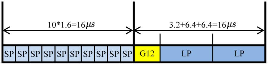
Format of IEEE 802.11p PHY layer.

The corresponding OFDM symbol is

s (t) = w (t) \sum_{k = - N / 2}^{k = N / 2} S_{k} \exp (j 2 π k Δ_{F} t)

(3)

where N = 52 and $w (t)$ is the window function of the SP. The factor $\sqrt{13 / 6}$ normalizes the average power of the OFDM symbol as it uses only 12 subcarriers. Because S has nonzero values only for indices that are a multiple of 4, the SP symbol duration is T_FFT/4 = 1.6 µs. Thus, the SP symbols have a duration of 16 µs.

Each LP symbol consists of 52 nonzero subcarriers and 12 null subcarriers with a duration of 6.4 µs. Between the SPs and LP are two GI symbols (each of duration 1.6 µs). Thus, the preamble has duration of 10 × 1.6 µs+2 × 1.6 µs+2 × 6.4 µs = 32 µs.

The preamble is used for time and frequency synchronization as well as channel estimation. The short symbols are typically used for coarse time estimation of the signal and the long symbols are used for fine estimation. The coarse time estimation is critical to the success of the fine estimation and so is considered in this article.

Channel

In most cases, the send signal may be reflected, scattered, or diffracted by different objects, which may cause a number of different paths and introduce the LOS or NLOS to the channel between transmitter and receiver. To date, there is no generally accepted model for vehicular channels. However, the AWGN channel has long been employed as a baseline for communication systems, while the Rician model for LOS multipath channels and the Rayleigh model for NLOS multipath channels are commonly used. At the same time, ITU vehicular test environment¹⁰ can be used to model the multipath delays and channel gains. The recommendation specifies two different delay spreads: low delay spread (A) and medium delay spread (B). The simulation in this article uses Channel A which has six taps with power gains 0, −1, −9, −10, −15, and −20 dB and relative delays 0, 310, 710, 1090, 1730, and 2510 ns. The received OFDM signal in the time domain is affected by phase noise $Φ (t)$ and AWGN $w (t)$ , so it can be expressed as

r (t) = s (t) \exp (j Φ (t)) + w (t)

(4)

Timing estimation methods

Normally speaking, in the receiver, the signal is correlated with the corresponding reference template signal. The correlation function is defined as follows

r_{xs} (τ_{d}) = \frac{1}{T_{0}} \int_{T_{0}} p (t) r (t - τ_{d}) dt

(5)

where T₀ is the correlation duration, p(t) is the reference template signal, and r(t) is the received signal.

Receiver can calculate the propagation delay or the time offset according to the position of the maximum output signal from the correlator. Thus, time offset estimation is used to calculate the vehicle ranging by multiplying the speed of electromagnetic wave. So, the inaccurate time offset may cause inaccurate vehicle ranging estimation. Several techniques have been developed for OFDM-based coarse time estimation.

Well-known methods

In OFDM, the time estimation algorithms do not need to estimate the exact packet start point and sometime error is allowed if the whole multipath channel is covered by the CP. Therefore, if offset estimation is used to calculate the vehicle ranging, more accurate time estimation is required. Obviously, using all the SP samples has better performance than using less SP samples, yet it requires more computational load. To reduce the complexity, a lot of suboptimal algorithms are proposed.

SC method

In the SC method,¹³ the preamble pattern in the time domain is [GI A A], so that after the GI, the symbol in the first half is the same as that in the second half. The GI is the same as the last part of symbol. The SC method uses the following timing metric

M (d) = \frac{{| P (d) |}^{2}}{R^{2} (d)}

(6)

where P(d) and R(d) are the auto-correlation and energy of the received signal r, respectively, given by

P (d) = \sum_{m = 0}^{L - 1} r^{*} (d + m) \cdot r (d + m + L)

(7)

R (d) = \sum_{m = 0}^{L - 1} {| r (d + m + L) |}^{2}

(8)

where L is the length of r, d is the time index corresponding to the received samples, and * denotes complex conjugate. Thus, there are N = 2L training samples.

Figure 2 presents |P(d)|², R²(d), and M(d) with L = 32 for an ideal channel without noise and a time delay of 191 samples. For the IEEE 802.11p structure, the length of the SPs is 160 samples, so the first 160 − 2L = N_g = 96 samples are considered to be the GI. This shows that the timing metric forms a plateau which has a length equal to the length of the GI (N_g = 96 samples) minus the length of the channel delay spread. In an AWGN channel, there is no delay spread, so the length of the plateau is 96 samples.

Figure 2.

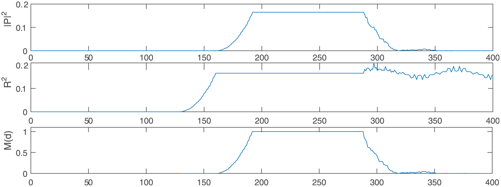
|P(d)|², R²(d), and M(d) of SC method with L = 32 in ideal environment.

The plateau with the SC method results in uncertainty in the timing estimation. As the length of the SPs is 160 samples, N_g = 0 is required to eliminate the plateau, which gives L = 80.

Reddy–Mahanta–Bora method

In order to overcome the uncertainty leaded by the plateau in SC method, Reddy et al.¹⁶ have given a modification to the timing metric of equation (6), as shown in equation (9)

K (d) = M (d) - M (d - L)

(9)

Here, there is no plateau in K(d). As shown in Figure 3, an example of timing metric M(d) of SC and K(d) of Reddy–Mahanta–Bora (RMB) method is simulated in an AWGN channel with E_b/N₀ (the energy per bit to noise power spectral density ratio) = 30 dB, time delay = 191 samples, and L = 16.

Figure 3.

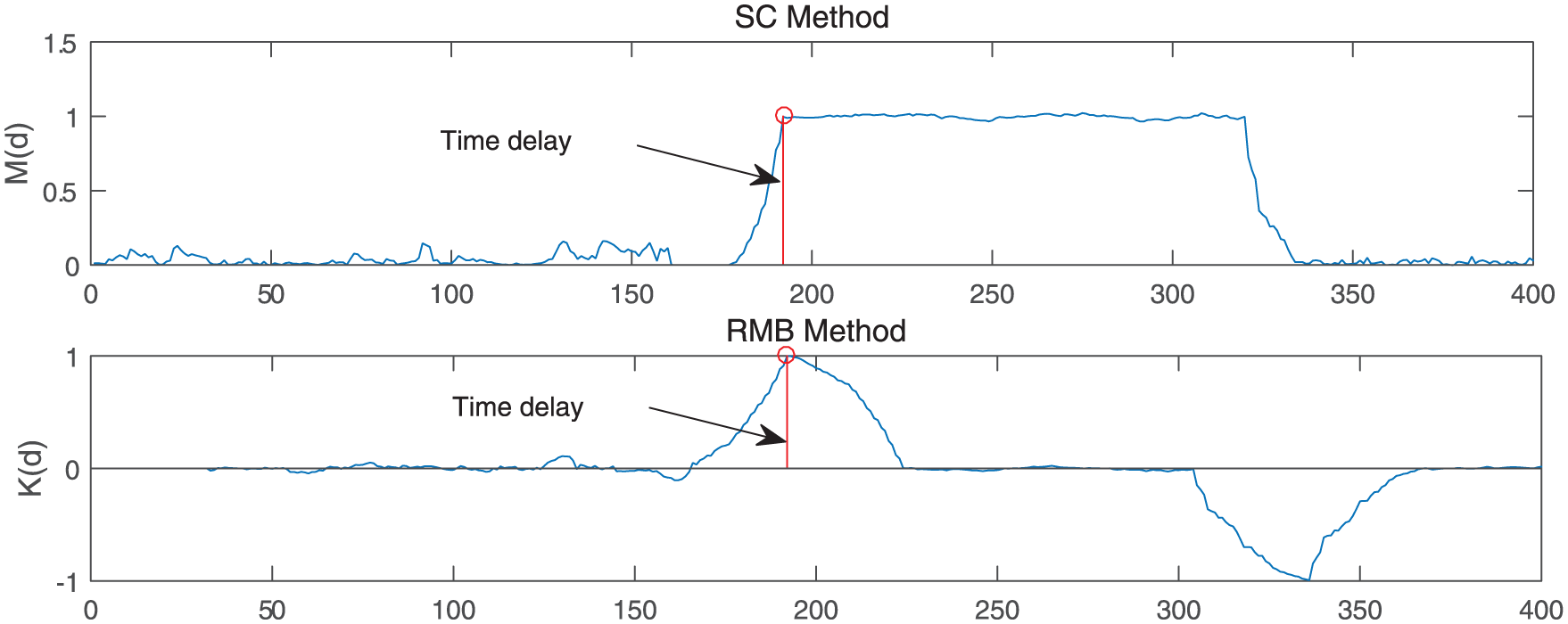
M(d) of SC method and K(d) of RMB method.

MZB method

The MZB timing metric is averaged over a window of length N_g+1 samples which is given by

M_{1} (d) = \frac{1}{N_{g} + 1} \sum_{k = - N_{g}}^{0} M (d + k)

(10)

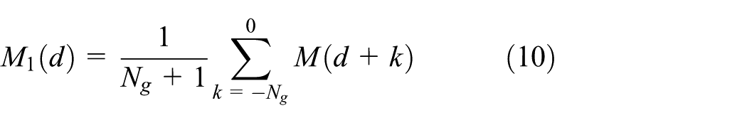
where N_g is the length of the GI, M(d) is the same as in equation (6), and P(d) is the same as in equation (7), but R(d) is given by

R (d) = \frac{1}{2} \sum_{m = 0}^{N - 1} {| r (d + m) |}^{2}

(11)

where N is the number of training samples N = 2L. Figure 4 shows |P(d)|², R²(d), and M₁(d) for the MZB method with N_g = 96, N = 64, and L = 32 in an ideal channel with a time delay of 191 samples. Compared to Figure 2, there is no plateau, but the peak is parabolic and is not very sharp.

Figure 4.

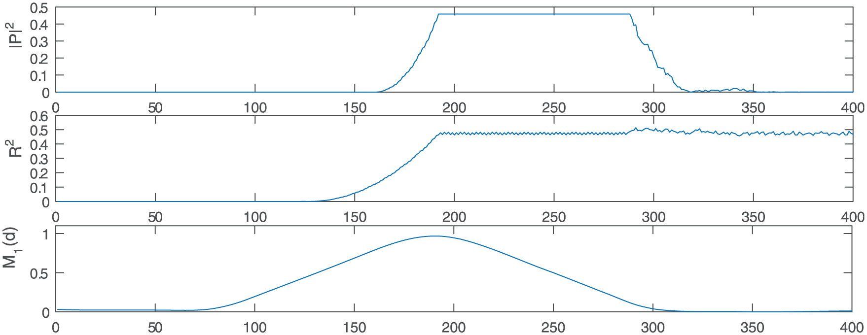
|P(d)|², R²(d), and M(d) for the MZB method in ideal environment.

MathWorks method

The SC, RMB, and MZB methods all use the auto-correlation of the received signal, but in the software of MATLAB, MathWorks¹⁷ method employs a cross-correlation between the received signal and the known SP given in equation (2). The timing metric M(d) is the same with the SC method as shown in equation (6), but P(d) and R(d) are defined as

P (d) = \sum_{m = 0}^{L - 1} r (d + m) \cdot t^{*} (1 + m)

(12)

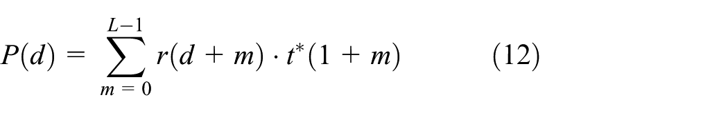
and

R (d) = \sum_{m = 0}^{T - 1} {| r (d + m) |}^{2}

(13)

where t(1+m) is the SP sequence, that is, the reference template, with length T = 16. During the timing period, the 60% of the maximum of normalized M is used as a threshold to choose the peaks from M. If the peaks exceeding the threshold are located in the spacing of 16 times (16, 32, 48, …, 128) and the count of these peaks is more than 5, the location of the first peak $(L_{first})$ is deemed as the peak of the first path, and the delay $({\hat{D}}_{est})$ is estimated as

{\hat{D}}_{est} = L_{first} - (\frac{L}{2} + 1)

(14)

Two examples of timing metric M(d) are simulated in Figure 5 with time delay = 191 samples and E_b/N₀ = 0 dB and 30 dB, respectively. In these cases, the first peak should be located at L_first = 191+16/2+1 = 200th samples. As shown in Figure 5, when E_b/N₀ = 30 dB, the nine peaks are very sharp and the first peak appears at 200th sample, as expected. When E_b/N₀ = 30 dB, all nine peaks exceed the threshold, but when E_b/N₀ = 0 dB, there are only two peaks exceeding the threshold, so the timing offset cannot be estimated accurately. In order to solve this problem, a further step is put forward in section “Proposed method.”

Figure 5.

M(d) of MathWorks method in different E_b/N₀.

Proposed method

The main steps of the proposed method contain correlation, sum, and deviation.

Correlation

The first step, named as correlation, is the same as MathWorks method. As shown in Figure 5, in an ideal environment, M(d) will have nine peaks, and the spacing between each adjacent desired peak will be 16 samples. However, if E_b/N₀ is low, the noise can affect the number of peaks that exceeds the threshold, and it is difficult to determine the optimal threshold value.

Sum

The sum of nine values of M(d) spaced T = 16 samples apart is considered, as shown in equation (15)

G (t) = \sum_{d = 1}^{9} M (t + (d - 1) * L)

(15)

and the time delay $({\hat{D}}_{est})$ estimate is obtained as

{\hat{D}}_{est} = \arg max (G (t)) - (\frac{T}{2} + 1)

(16)

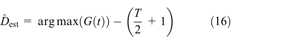
In ideal environment with no noise, the group-sum G(t) is simulated in Figure 6 with time delay = 191 samples. Now, there are 17 symmetrical peaks and the location of the maximum peak is just the position to be found, which should be located at 191+16/2+1 = 200.

Figure 6.

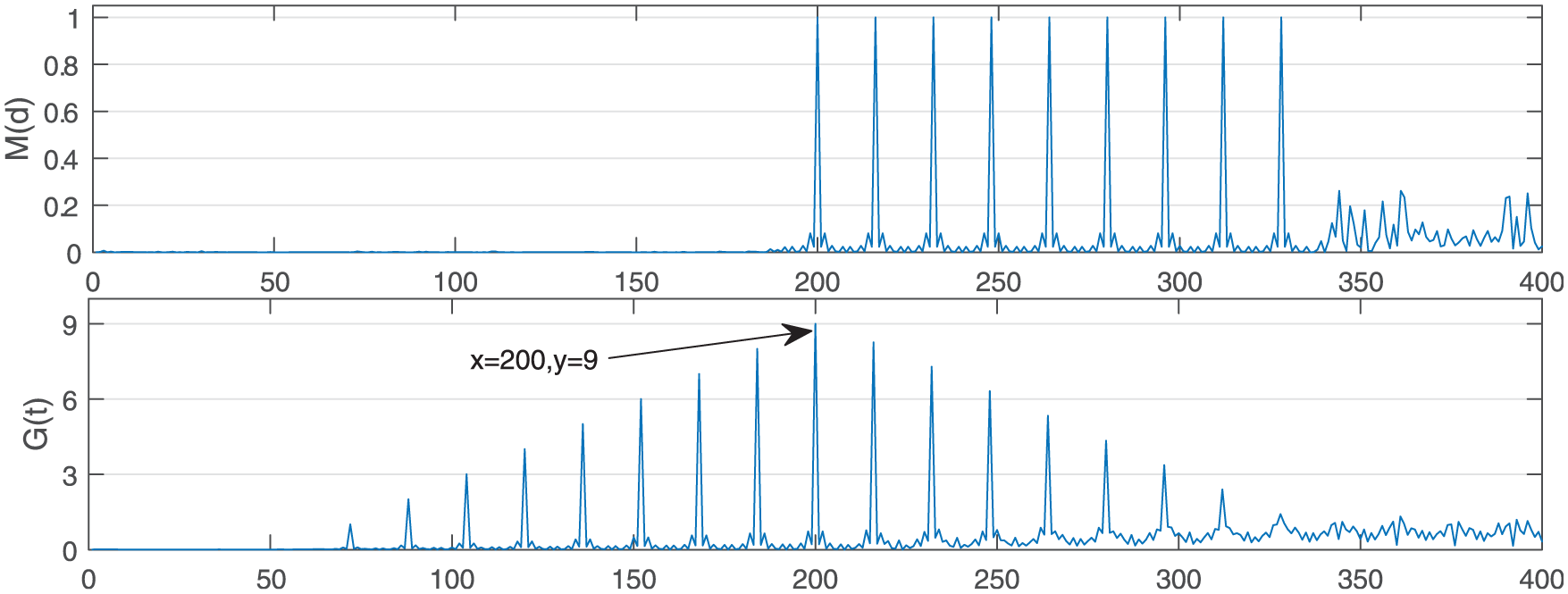
M(d) and G(t) in ideal environment.

As E_b/N₀ decreases, the M(d) of MathWorks method becomes more and harder to be identified, but the group-sum G(t) is better. As shown in Figure 7, when E_b/N₀ = −5 dB, the nine peaks of M(d) are very hard to be identified, but the maximum of G(t) is very clear and appears at 200th sample, and then the time delay ${\hat{D}}_{est}$ can be estimated correctly. Generally speaking, the sum of the desired peaks may be higher than the others.

Figure 7.

M(d) and G(t) with E_b/N₀ = −5 dB.

However, as E_b/N₀ decreases more and more, the G(t) will turn more difficult to be identified. As shown in Figure 8, when E_b/N₀ = −10 dB, the maximum of G(t) is very hard to be located at 200th sample, and then the time delay ${\hat{D}}_{est}$ cannot be estimated correctly.

Figure 8.

G(t) with E_b/N₀ = −10 dB.

Deviation

In order to improve the precise in low E_b/N₀, standard deviation (STD) of the adjacent 16 G (stdG) is given by Figure 9 and the time delay $({\hat{D}}_{est})$ estimated may be obtained by

{\hat{D}}_{est} = PeakIndex - (\frac{T}{2} + 1)

(17)

Figure 9.

G(t) and stdG in ideal environment.

In ideal environment with no noise, the stdG is simulated in Figure 9 with time delay = 191 samples. Now, there are 12 stdGs, and stdG[1] = 1 is the normalized STD from the data of G[184] to G[199], stdG[2] =0.8747 from G[168] to G[183], stdG[3] = 0.7495 from G[152] to G[167], …, and so on. It is shown that the stdGs before 10 nearly form a straight line. At the same time, stdG[1] = 1 and stdG[10] = 0 which can be used as a metric to check whether the PeakIndex is corresponding to the time estimation.

However, when E_b/N₀ is very low, for example, −10 dB, the PeakIndex = argmax(G) is not located at the sample corresponding to the delay time. As shown in Figure 10, PeakIndex should be located at 200th sample, but actually it is at 300th. The stdG before iteration shows that stdG[1] is <1, and stdG[10] = 0.57 is >0, as shown in Figure 9.

Figure 10.

G(t) and stdG with E_b/N₀ = −10 dB.

The deviation iteration is used to make sure that stdG[1] > 0.9 and stdG[10] < 0.1, as shown in the flow chart of Figure 11. If stdG[1] < 0.9 or stdG[10] > 0.1, there will be an iteration to set G[PeakIndex] = 0, to find the next PeakIndex, then to compute new stdGs, and then to check stdG[1] or stdG[10] again, until the length of stdG is <10 or stdG[1] > 0.9 and stdG[10] < 0.1. The simulation of stdG after deviation iteration is shown in Figure 10, and now the PeakIndex is correctly located at 200th sample.

Figure 11.

Flow chart of the deviation iteration.

Performance results and discussion

In this section, the performance and complexity of the proposed method are examined in AWGN channels and Rician channels with the ITU Channel A parameters. The performance metrics employed are mean absolute errors (MAE) and P(x)

MAE = \frac{1}{K} \sum_{n = 1}^{K} | D_{n} - {\overset{⌢}{D}}_{n} |

(18)

where D_n is the peak index corresponding to the nth actual time delay, ${\overset{⌢}{D}}_{n}$ is the peak index corresponding to the nth estimated time delay, and K is the number of simulation iterations

P (x) = \frac{1}{K} CountIF (| {\hat{D}}_{n} - D_{n} | \leq x)

(19)

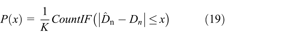
where CountIF is the number of times the estimated error is not larger than a given value x. For example, P(0) is the average number of times the estimate is correct.

Because vehicles are typically in motion, there will be a Doppler shift given by

F_{d} = v \times \frac{f_{c}}{c}

(20)

where v is the maximum relative vehicle speed which is typically set to v = 100 km/h, f_c = 5.9 GHz is the center frequency of the transmitted signal, and c is the speed of light. Carrier frequency offset is unavoidable in practice and hence it is included in the performance evaluation.

The SC method with L = 32 (denoted SC-32) has a plateau as shown in Figure 2, so the timing estimation is difficult. To mitigate this problem, L = 80 is used (denoted SC-80). The timing metric of SC-80 is presented in Figure 12 for an ideal environment with a time delay of 191 samples, and this indicates that there is now no plateau, but the number of values required for the correlation is over twice that of the other methods, so the complexity is higher.

Figure 12.

|P(d)|², R²(d), and M(d) of SC-80 method in ideal environment.

In the remainder of this article, six methods are considered: MathWorks, the proposed method, SC-32, SC-80, RMB, and MZB.

AWGN channel performance

The performance in AWGN channel was simulated K = 2000 times for values of E_b/N₀ from −15 to 20 dB. Figure 13 presents MAE for the six methods. These results show that the proposed method provides the best performance, particularly at low to moderate signal-to-noise ratio (SNR) values. For example, when E_b/N₀ = −9 dB, the MAE of the proposed method is 6.6 samples, while MAE are only 87 samples for MZB and SC-80, 128 samples for SC-32 and RMB, and 192 samples for MathWorks. When E_b/N₀ is <2 dB, the MAE of MathWorks is the highest and when E_b/N₀ is >2 dB, the MAE of SC-32 is the highest.

Figure 13.

MAE of different methods in AWGN channel.

Figure 14 presents P(0) for the six methods. These results also show that the proposed method provides the best performance. For example, when E_b/N₀ = −6 dB, the P(0) of the proposed method provides 85%, while all the other methods are <7%. For E_b/N₀ = 0 dB, the percentage of time the proposed method had no error is 98%, whereas for the same percentage with MathWorks, E_b/N₀ should exceed 9 dB; with SC-80, E_b/N₀ should exceed 11 dB; with MZB, E_b/N₀ should exceed 18 dB; and for RMB and SC-32, the percentage are lower for all values of E_b/N₀.

Figure 14.

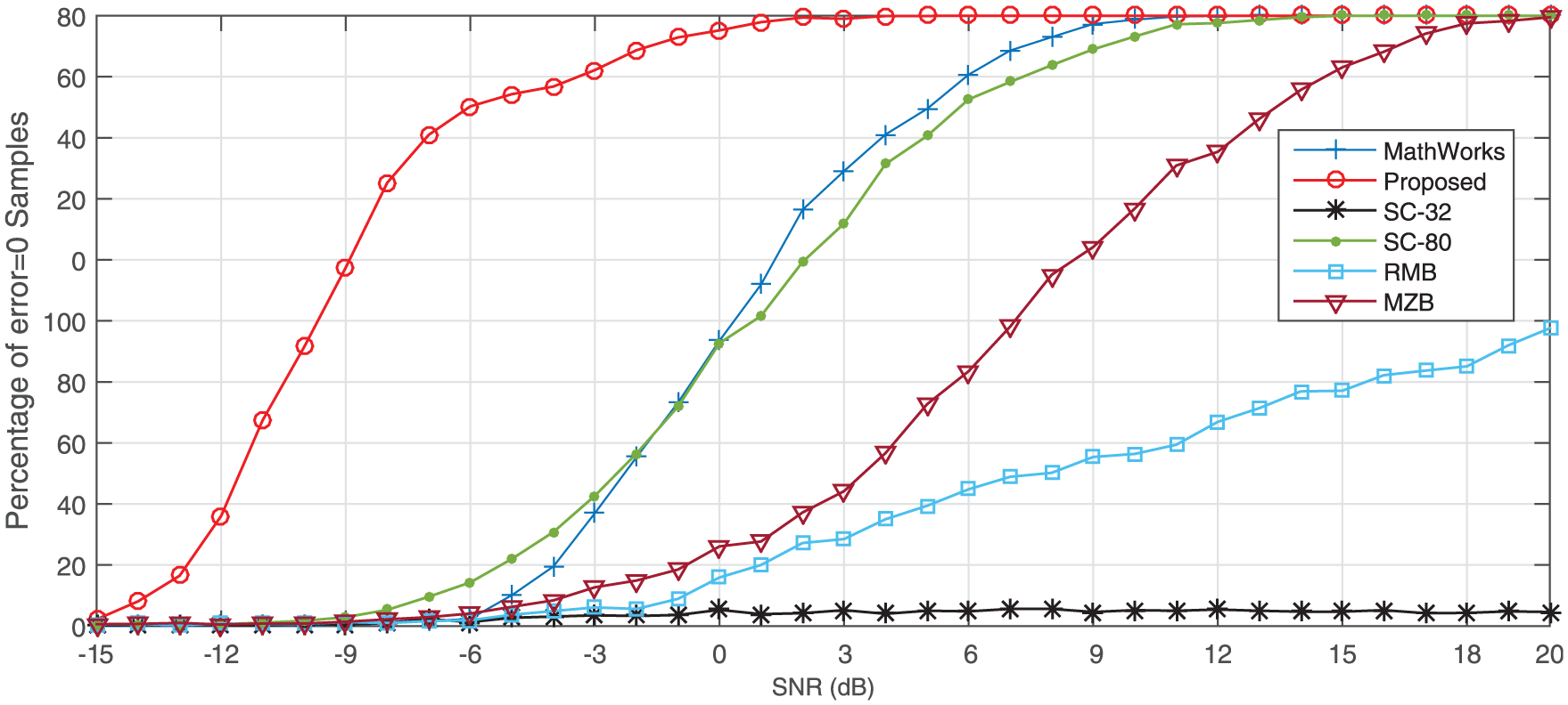
Probability that the timing error is zero in AWGN channel.

Figure 15 presents P(3) for the six methods. This shows that the proposed method again has the best performance. Furthermore, the results for the proposed method in Figures 14 and 15 are almost the same, but differ significantly for the other methods. When E_b/N₀ = 0 dB, P(3) with the proposed method is nearly 98%, but for the same percentage with SC-80, E_b/N₀ should be greater than 5 dB; with MZB and MathWorks, E_b/N₀ should exceed 10 dB; with RMB, E_b/N₀ should be greater than 18 dB; and with SC-32, the P(3) is never greater than 10%.

Figure 15.

Probability that the timing error is less than three samples in AWGN channel.

Multiple path performance

The Rician channel with ITU vehicular Channel A parameters was simulated K = 2000 times for values of E_b/N₀ from −10 to 20 dB. There are six paths, with the gains and delays given in section “System model.”

Figure 16 presents MAE for the six methods in multipath environment. Table 1 shows that all the MAEs of different methods in ITU multiple path channel are lower than those in AWGN channel of Figure 14, but the proposed method provides the best performance in both AWGN and ITU multiple path channel.

Figure 16.

MAE of different methods in ITU vehicular Channel A.

Table 1.

MAEs of different methods in different channels.

Methods	AWGN			ITU vehicular Channel A
Methods	−10 dB	0 dB	10 dB	−10 dB	0 dB	10 dB
MathWorks	191.90	79.22	0.28	192.00	179.73	9.06
Proposed	9.86	0.38	0.00	37.75	2.25	0.28
SC-32	128.82	47.06	47.84	136.16	51.58	52.76
SC-80	98.20	1.90	0.04	101.64	3.92	2.99
RMB	133.44	23.82	2.24	135.60	31.56	5.12
MZB	96.57	5.65	0.53	102.59	5.75	1.74

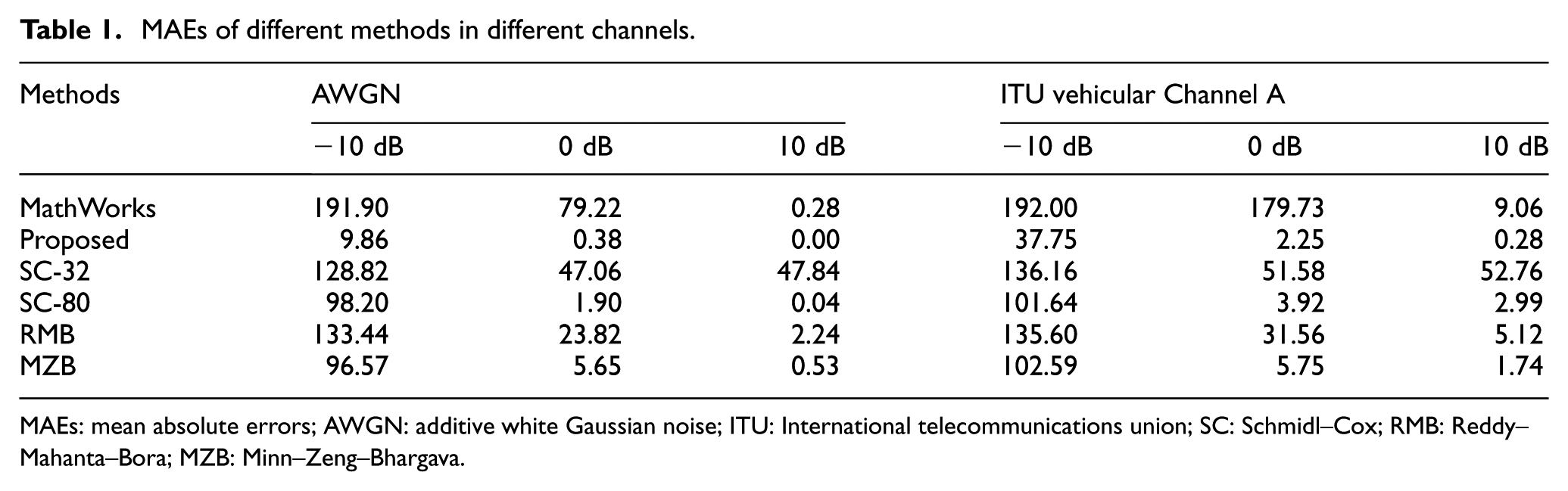
MAEs: mean absolute errors; AWGN: additive white Gaussian noise; ITU: International telecommunications union; SC: Schmidl–Cox; RMB: Reddy–Mahanta–Bora; MZB: Minn–Zeng–Bhargava.

Figure 17 presents P(0) for the four methods. This shows that only the proposed method provides adequate performance and when E_b/N₀ is higher than 13 dB, MathWorks method can reach nearly 100%. However, for the other methods, P(0) increases at first as E_b/N₀ increases, and then decreases to a value near 0. The reason for the behavior is as follows:

When E_b/N₀ is high, the multiple signal paths cause the time metrics to move to the right, so the timing estimates will be incorrect. Take MZB and SC methods as examples, which are illustrated in Figure 18 for the multipath channel with no noise. Therefore, P(0) will be close to 0. However, Figure 19 shows that time metrics of the proposed method do not move, so P(0) will be nearly equal to 100% for a high SNR.

When E_b/N₀ is very low (nearly −10 dB), the noise levels are high, so it is very difficult to locate the peak, so P(0) is again near to 0.

For E_b/N₀ around 0 dB, the signal energy is near that of the noise, so it is easier to locate the peak. Now because of the randomization of noise, it is likely that the estimated time happens to be right.

Figure 17.

Probability that the timing error is zero in ITU vehicular Channel A.

Figure 18.

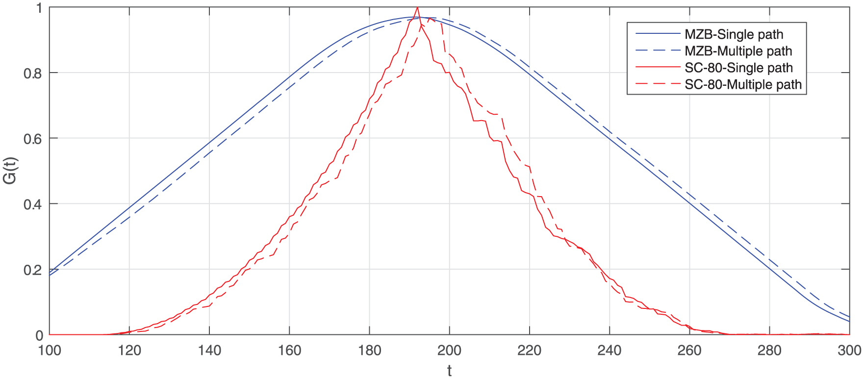
The effect of the multipath channel on the timing estimates of the MZB and SC methods.

Figure 19.

The effect of the multipath channel on the timing estimates of the proposed method.

Figure 20 presents P(3) for the six methods in the multipath channel. This shows that when E_b/N₀ is sufficiently large, the proposed method is the best, which can reach P(3) = 100% at the E_b/N₀ of 6 dB, and then the MZB, MathWorks, and SC-80 methods, which can reach P(3) = 100% at the E_b/N₀ of 12 dB. However, the performance of RMB and SC-32 is poor for all SNR values. With E_b/N₀ is small, the proposed method has the best performance, followed by the SC-80 and MZB methods.

Figure 20.

Probability that the timing error is less than three samples in ITU vehicular Channel A.

Complexity and efficiency

Although the time complexity of different methods seems like the same, they all have the order of n² time complexity, that is, O(n²) using big O notation; however, the running time is not the same actually.

Although the time complexity of the methods is O(n²), the running time differs significantly. The most complex operation is the correlation, so SC-80 has the higher complexity because the number of samples used in the correlation is 80, whereas this number for the other methods is only 32. For the proposed method, the deviation iteration in low E_b/N₀ is an important factor which will cause higher complexity.

In order to compare the efficiency of different methods, 1000 iterations were performed for each value of E_b/N₀ from −13 to 1 dB, and the average time is given in Figure 21.

Figure 21.

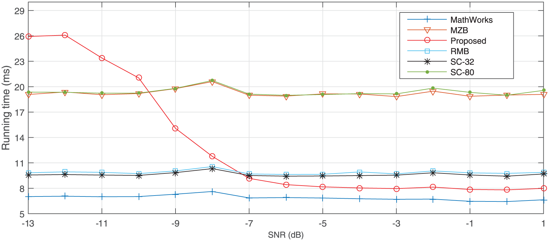
Comparison of running time for different methods.

Figure 21 shows that when SNRs are lower than −10 dB, the proposed method has the highest complexity because of the deviation iteration, but with these low SNRs, it is very difficult for other methods to estimate time successfully. As the SNRs increasing, the complexity of the proposed method decreases, but it is a little higher than the MathWorks method because of the deviation operation, whereas other four techniques have the highest complexity which is more than three times greater.

Conclusion

In this article, a low complexity, high precise ranging estimation method based on the SP has been developed for vehicular node positioning with IEEE 802.11p wireless communication. A new method based on the correlation-sum-deviation was developed for time offset estimation. The performance of the proposed method was shown to be the best among the several well-known methods in any different SNRs both with AWGN and with multipath ITU channels. Although its complexity is worse with low SNRs, however, now the other methods cannot estimate time at all, and with higher SNRs, its complexity decreased significantly.

Footnotes

Academic Editor: Zhipeng Cai

Declaration of conflicting interests

The author(s) declared no potential conflicts of interest with respect to the research, authorship, and/or publication of this article.

Funding

The author(s) disclosed receipt of the following financial support for the research, authorship, and/or publication of this article: This work was supported by the National Natural Science Foundation of China under grant no. 61301139, the Nature Science Foundation of Shandong Province No. ZR2014FL014, Distinguished Middle-Aged and Young Scientist Encourage and Reward Foundation of Shandong Province No. 2014BSE28032, the Fundamental Research Funds for the Central Universities No. 16CX02046A, and the Project of Basic Research Application of Qingdao City No. 14-2-4-83-jch.

References

World Health Organization (WHO). Global status report on road safety 2013: supporting a decade of action, 2013, http://www.who.int/violence_injury_prevention/road_safety_status/2013/en/

Wang

Guo

. An urban area-oriented traffic information query strategy in VANETs. In: 8th international conference on wireless algorithms, systems, and applications (WASA 2013), Zhangjiajie, China, 7–10 August 2013, pp.313–324. Zhangjiajie, China: Springer-Verlag.

Huang

Chen

Cai

. Graph theory based capacity analysis for vehicular Ad Hoc networks. In: 58th IEEE global communications conference (GLOBECOM 2015), San Diego, CA, 6–10 December 2015. San Diego, CA: Institute of Electrical and Electronics Engineers Inc.

Guan

Huang

Cai

. Intersection-based forwarding protocol for vehicular ad hoc networks. Telecommun Syst 2016; 62: 67–76.

Xiao

Bai

. Research on positioning enhancement scheme of CAPS via UWB pseudolite. Sci China: Phys Mech Astron 2012; 55: 733–737.

Ansari

Feng

Tang

ML.

A runtime integrity monitoring framework for real-time relative positioning systems based on GPS and DSRC. IEEE T Intell Transp 2015; 16: 980–992.

Huang

Guan

Cai

. Multicast capacity analysis for social-proximity urban bus-assisted VANETs. In: 2013 IEEE international conference on communications (ICC 2013), Budapest, 9–13 June 2013, pp.6138–6142. Budapest: Institute of Electrical and Electronics Engineers Inc.

IEEE 802.11p-2010 standard. IEEE Standard for Information technology—local and metropolitan area networks specific requirements—part 11: wireless LAN medium access control (MAC) and physical layer (PHY) specifications amendment 6: wireless access in vehicular environments.

IEEE 802.11a-1999 standard, http://standards.ieee.org/getieee802/download/802.11a-1999.pdf (accessed 30 August 2015).

10.

Guidelines for evaluation of radio transmission technologies for IMT-2000, https://www.itu.int/oth/R0A0E00000C/en (accessed 30 August 2015).

11.

Parker

Valaee

Vehicular node localization using received-signal-strength indicator. IEEE T Veh Technol 2007; 56: 3371–3380.

12.

Sun

Zhang

. A frame synchronization and symbol timing synchronization algorithm in burst OFDM communication based on IEEE802.11a. In: International forum on information technology and applications (IFITA ’09), Chengdu, China, 15–17 May 2009, pp.190–193. New York: IEEE.

13.

Schmidl

Cox

DC.

Robust frequency and timing synchronization for OFDM. IEEE T Commun 1997; 45: 1613–1621.

14.

Oni

RRA

. Preamble design problematic with 802.11a IEEE standard (Minn’s training sequence). Radioengineering 2008; 17: 87–91.

15.

Minn

Zeng

Bhargava

VK.

On timing offset estimation for OFDM systems. IEEE Commun Lett 2000; 4: 242–244.

16.

Reddy

Mahanta

Bora

. On timing and frequency offset estimation in OFDM systems. In: TENCON 2004: 2004 IEEE region 10 conference, Chiang Mai, Thailand, 21–24 November 2004, vol. 153, pp.153–156. New York: IEEE.

17.

MathWorks. OFDM synchronization, http://www.mathworks.com/help/comm/examples/ofdm-synchronization.html (accessed 30 August 2015).

Correlation-sum-deviation ranging method for vehicular node based on IEEE 802.11p short preamble

Abstract

Keywords

Introduction

System model

Introduction

OFDM symbol

Preamble symbol

Channel

Timing estimation methods

Well-known methods

SC method

Reddy–Mahanta–Bora method

MZB method

MathWorks method

Proposed method

Correlation

Sum

Deviation

Performance results and discussion

AWGN channel performance

Multiple path performance

Complexity and efficiency

Conclusion

Footnotes

Declaration of conflicting interests

Funding

References