Sage Journals: Discover world-class research

Abstract

In this article, we develop a command, xthenreg, that implements the first-differenced generalized method of moments estimation of the dynamic panel threshold model that Seo and Shin (2016, Journal of Econometrics 195: 169–186) proposed. Furthermore, we derive the asymptotic variance formula for a kink-constrained generalized method of moments estimator of the dynamic threshold model and provide an estimation algorithm. We also propose a fast bootstrap algorithm to implement the bootstrap for the linearity test. We illustrate the use of xthenreg through a Monte Carlo simulation and an economic application.

Keywords

st0573 xthenreg dynamic panel threshold model

1 Introduction

The panel model with threshold effects in Hansen (1999) has been widely used in empirical research. Hansen’s fixed-effects estimator has been applied to applications on the investment decision of firms under financial constraints, the relation between a fiscal deficit and economic growth (Adam and Bevan 2005), the relation between inflation and growth (Khan and Ssnhadji 2001), and others. The threshold effect in the model allows for the asymmetric effect of the exogenous variables, depending on whether the threshold variable is above or below the unknown threshold. The threshold variable is typically dictated by the economic model. For instance, in the investment decision problem, the size of the firm is often considered a candidate threshold variable. Wang (2015) developed a command, xthreg, that computes Hansen’s estimator.

Hansen’s (1999) model is static, and his fixed-effects estimator requires the covariates to be strongly exogenous for the estimator to be consistent. However, strong exogeneity can be restrictive in many real applications. Thus, the model has been extended to the dynamic panel model with a potentially endogenous threshold variable as proposed by Seo and Shin (2016). Their model allows lagged dependent variables and endogenous covariates. Indeed, various applications of Hansen’s fixed-effects estimation can benefit from dynamic modeling. For instance, the investment decision depends on the previous period’s investment, and the panel threshold autoregressive model is another example of dynamic models.

We developed commands for the first-differenced generalized method of moments (GMM) estimators and the associated asymptotic variance estimator that are proposed by Seo and Shin (2016) as well as linearity testing for the presence of a threshold effect. While the previous command xthreg computes the fixed-effect estimator and thus is not consistent under this general setting, our command xthenreg produces consistent and asymptotically normal estimates.

We also propose a computationally more attractive bootstrap algorithm to implement the linearity test than the nonparametric independent and identically distributed bootstrap that was originally proposed by Seo and Shin (2016). Furthermore, we present a constrained GMM estimator that reflects the kink restriction that has become more popular in recent years—see, for example, Zhang, Zhou, and Jiang (2017)— along with its asymptotic variance formula and a consistent estimator.

This article is organized as follows: Section 2 introduces the dynamic threshold panel model and the first-differenced GMM estimator. It also presents the asymptotic variance formula for a kink-constrained estimator and a bootstrap algorithm for the linearity test. Section 3 explains the command xthenreg. Sections 4 and 5 illustrate its use through Monte Carlo simulations and an application. Section 6 concludes.

2 Model

The dynamic panel threshold model is given by

y_{i t} = x_{i t}^{'} β + (1, x_{i t}^{'}) δ 1 {q_{i t} > γ} + μ_{i} + ε_{i t} i = 1, . . ., n; t = 1, . . ., T

where x _it may include lagged dependent variables and q_it is the threshold variable. We assume T is fixed while the sample size n grows to infinity. Thus, we remove the incidental parameter µ_i with the first-difference transformation and estimate the unknown parameters θ = (β′, δ ′, γ)′ through the GMM. The following describes the GMM method from Seo and Shin (2016).

Specifically, set an l-dimensional vector of instrument variables, (z′it ₀, …, z′ _iT )′, from the lagged variables and exogenous variables, where 2 < t ₀ ≤ T . Next, construct the sample moment

{\bar{g}}_{n} (θ) = {\bar{g}}_{1 n} - {\bar{g}}_{2 n} (γ) {(β^{'}, δ^{'})}^{'} = \frac{1}{n} \sum_{i = 1}^{n} g_{1 i} - \frac{1}{n} \sum_{i = 1}^{n} g_{2 i} (γ) {(β^{'}, δ^{'})}^{'}

where

g_{1 i} = (\begin{array}{l} z_{i t_{0}} Δ y_{i t_{0}} \\ ⋮ \\ z_{i t_{0}} Δ y_{i t_{0}} \end{array}), g_{2 i} (γ) = (\begin{array}{l} z_{i t_{0}} (Δ {x^{'}}_{i t_{0}}, 1_{i t_{0}} {(γ)}^{'} X_{i t_{0}}) \\ ⋮ \\ z_{i T} (Δ {x^{'}}_{i T}, 1_{i T} {(γ)}^{'} X_{i T}) \end{array}),

with Δ signifying the first-difference operator and

X_{i t} = (\begin{array}{l} (1, {X^{'}}_{i t}) \\ (1, {X^{'}}_{i,t - 1}) \end{array}) and 1_{\begin{array}{l} i t \\ 2 \times 1 \end{array}} (γ) = (\begin{array}{l} 1 {q_{i t} > γ} \\ - 1 {q_{i t} - 1 > γ} \end{array})

Then, introduce the GMM criterion function with a weight matrix W _n,

{\bar{J}}_{n} (θ) = {\bar{g}}_{n} {(θ)}^{'} W_{n} {\bar{g}}_{n} (θ)

which is minimized to produce a GMM estimate, $\hat{θ}$ .

The minimization is done by the grid search because for each fixed γ the model becomes a linear panel with a fixed effect, which yields the closed-form solution

{\hat{β} {(γ)}^{'}, \hat{δ} {(γ)}^{'}}^{'} = {{\bar{g}}_{2 n} {(γ)}^{'} W_{n} {\bar{g}}_{2 n} (γ)}^{- 1} {\bar{g}}_{2 n} {(γ)}^{'} W_{n} {\bar{g}}_{1 n}

and the criterion function ${\bar{J}}_{n} (θ)$ is a step function over γ with at most nT jumps. However, note that this algorithm is different from splitting the sample in two and applying the linear GMM for each partitioned sample.

For the weight matrix, either W _n = I _l or

W_{n} = {(\begin{matrix} \frac{2}{n} \sum_{i = 1}^{n} z_{i t_{0}} {z^{'}}_{i t_{0}} & \frac{- 1}{n} \sum_{i = 1}^{n} z_{i t_{0}} {z^{'}}_{i t_{0}} + 1 & 0 & \dots \\ \frac{- 1}{n} \sum_{i = 1}^{n} z_{i t_{0} + 1} {z^{'}}_{i t_{0}} & \frac{2}{n} \sum_{i = 1}^{n} z_{i t_{0} + 1} {z^{'}}_{i t_{0}} + 1 & ⋱ & ⋱ \\ 0 & ⋱ & ⋱ & \frac{- 1}{n} \sum_{i = 1}^{n} z_{i T - 1} {z^{'}}_{i T} \\ ⋮ & ⋱ & \frac{- 1}{n} \sum_{i = 1}^{n} z_{i T} {z^{'}}_{i T - 1} & \frac{2}{n} \sum_{i = 1}^{n} z_{i T} {z^{'}}_{i T} \end{matrix})}^{- 1}

was proposed in the first step, and it is updated to

W_{n} = {(\frac{1}{n} \sum_{i = 1}^{n} {\hat{g}}_{i} {\hat{g}}^{'}_{i} - \frac{1}{n^{2}} \sum_{i = 1}^{n} {\hat{g}}_{i} \sum_{i = 1}^{n} {\hat{g}}^{'}_{i})}^{- 1}

where ${\hat{g}}_{i} = {({\hat{Δ ε}}_{i t_{0}} {z^{'}}_{i t_{0}}, . . ., {\hat{Δ ε}}_{i T} {z^{'}}_{i T})}^{'} and {\hat{Δ ε}}_{i t}$ is the residual from the first-step estimation.

Seo and Shin (2016) showed that under suitable regularity conditions,¹ the GMM estimator is asymptotically normal. Specifically,

(\begin{array}{l} \sqrt{n} (\begin{array}{l} \hat{β} - β_{0} \\ \hat{δ} - δ_{n} \end{array}) \\ n^{\frac{1}{2 - α}} (\hat{γ} - γ_{0}) \end{array}) \overset{d}{\to} N {0, {(G^{'} Ω^{- 1} G)}^{- 1}}

where G = {G _β , G _δ (γ ₀) , G _γ (γ ₀)} with

\underset{l \times k_{1}}{G_{β}} = [\begin{array}{l} - E (z_{i t_{0}} Δ {x^{'}}_{i t_{0}}) \\ ⋮ \\ - E (z_{i T} Δ {x^{'}}_{i T}) \end{array}], \underset{l \times (k_{1} + 1)}{G_{δ} (γ)} = [\begin{array}{l} - E {z_{i t_{0}} 1_{i t_{0}} {(γ)}^{'} X_{i t_{0}}} \\ ⋮ \\ - E {z_{i T} 1_{i T} {(γ)}^{'} {x^{'}}_{i T}} \end{array}]

and

\underset{l \times 1}{G_{γ}} (γ) = [\begin{matrix} \begin{array}{l} [E_{t_{0} - 1} {z_{i t_{0}} (1, {x^{'}}_{i t_{0} - 1}) | γ} p_{t_{0} - 1} (γ) - E_{t_{0}} {z_{i t_{0}} (1, {x^{'}}_{i t_{0}}) | γ} p_{t_{0}} (γ)] δ_{0} \\ ⋮ \end{array} \\ [E_{T - 1} {z_{i T} (1, {x^{'}}_{i T - 1}) | γ} p_{T - 1} (γ) - E_{T} {z_{i T} (1, {x^{'}}_{i T}) | γ} p_{T} (γ)] δ_{0} \end{matrix}]

where E_t (·|γ) denotes the conditional expectation given q_it = γ and p_t (·) denotes the density of q_it .

The estimation of the asymptotic variance is standard; that is,

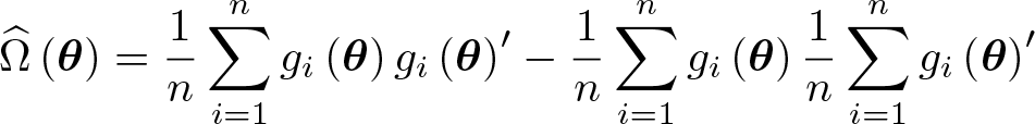
\hat{Ω} (θ) = \frac{1}{n} \sum_{i = 1}^{n} g_{i} (θ) g_{i} {(θ)}^{'} - \frac{1}{n} \sum_{i = 1}^{n} g_{i} (θ) \frac{1}{n} \sum_{i = 1}^{n} g_{i} {(θ)}^{'}

where g_i (θ) = g _1i + g _2i (γ) (β′, δ′)′ and

\begin{array}{l} {\hat{G}}_{β} = [\begin{matrix} - \frac{1}{n} \sum_{i = 1}^{n} z_{i t_{0}} Δ {x^{'}}_{i t_{0}} \\ ⋮ \\ - \frac{1}{n} \sum_{i = 1}^{n} z_{i T} Δ {x^{'}}_{i T} \end{matrix}], {\hat{G}}_{δ} (γ) = [\begin{matrix} - \frac{1}{n} \sum_{i = 1}^{n} z_{i t_{0}} 1_{i t_{0}} {(γ)}^{'} {X^{'}}_{i t_{0}} \\ ⋮ \\ - \frac{1}{n} \sum_{i = 1}^{n} z_{i T} 1_{i T} {(γ)}^{'} {X^{'}}_{i T} \end{matrix}] \\ {\hat{G}}_{γ} (θ) = [\begin{matrix} \frac{1}{n h} \sum_{i = 1}^{n} z_{i t_{0}} {{(1, {x^{'}}_{i t_{0} - 1})}^{'} K (\frac{γ - q_{i t_{0} - 1}}{h}) - {(1, {x^{'}}_{i t_{0}})}^{'} K (\frac{γ - q_{i t_{0}}}{h})} δ \\ ⋮ \\ \frac{1}{n h} \sum_{i = 1}^{n} z_{i T} {{(1, {x^{'}}_{i T - 1})}^{'} K (\frac{γ - q_{i T - 1}}{h}) - {(1, {x^{'}}_{i T})}^{'} K (\frac{γ - q_{i T}}{h})} δ \end{matrix}] \end{array}

which is the Nadaraya–Watson kernel estimator for some kernel K and bandwidth h, for example, the Gaussian kernel and Silverman’s rule of thumb. We plug in $θ = \hat{θ}$ .

2.1 Kink model

Although the threshold model typically implies the presence of a discontinuity of the regression function, it may mean the presence of a kink, not a jump, if (1, x′it) δ = κ (q_it − γ) for some κ. It happens when one element of x _it is q_it with the coefficient κ and the first element of δ equals to −γκ. Under these restrictions, the model becomes

y_{i t} = {x^{'}}_{i t} β + k (q_{i t} - γ) 1 {q_{i t} > γ} + α_{i} + ε_{i t} i = 1, . . ., n; t = 1, . . ., T

Even when the true model is a kink model, it is shown that the asymptotic distribution of the GMM estimator in the preceding section is valid. This contrasts with the least-squares estimator for the linear regression, for which Hidalgo, Lee, and Seo (2019) have shown that the cube root phenomenon appears.

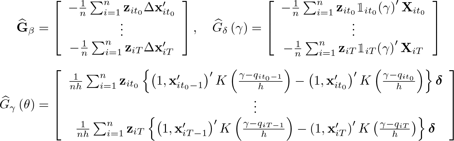
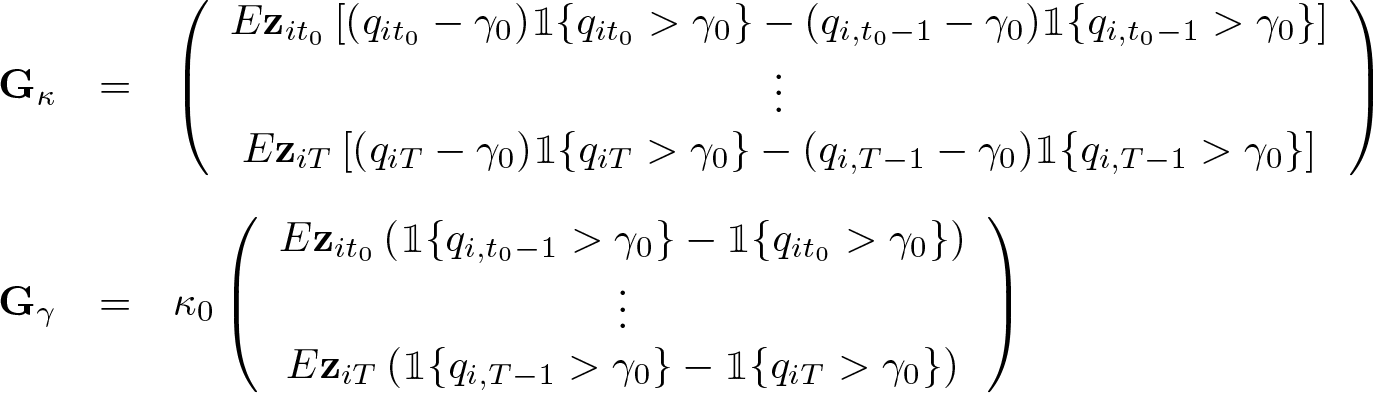
The asymptotic distribution of the constrained GMM estimator of (β, κ, γ) that imposes the kink restriction can also be derived for the same reason as Seo and Shin (2016). Specifically, the asymptotic variance is given by redefining G = (G _β, G _κ, G _γ ) , where G _β is the same as above and

\begin{array}{l} G_{k} = (\begin{matrix} E_{Z_{i t_{0}}} [(q_{i t_{0}} - γ_{0}) 1 {q_{i t_{0}} > γ_{0}} - (q_{i, t_{0} - 1} - γ_{0}) 1 {q_{i, t_{0} - 1} > γ_{0}}] \\ ⋮ \\ E_{Z_{i T}} [(q_{i T} - γ_{0}) 1 {q_{i T} > γ_{0}} - (q_{i, T - 1} - γ_{0}) 1 {q_{i, T - 1} > γ_{0}}] \end{matrix}) \\ G_{γ} = k_{0} (\begin{matrix} E_{Z_{i t_{0}}} [1 {q_{i t_{0} - 1} > γ_{0}} - 1 {q_{i, t_{0}} > γ_{0}}] \\ ⋮ \\ E_{Z_{i T}} [1 {q_{i T - 1} > γ_{0}} - 1 {q_{i, T} > γ_{0}}] \end{matrix}) \end{array}

The estimation of these terms is analogous to that of G _δ and G _γ in the preceding section.

2.2 Bootstrap test of linearity

This section proposes a fast bootstrap algorithm to test for the presence of the threshold effect, that is, the null hypothesis

H_{0} : δ_{0} = 0 for any γ \in Γ

where Γ denotes the parameter space for γ, against the alternative hypothesis

H_{1} : δ_{0} \neq 0 for some γ \in Γ

A standard approach is to use a supremum-type statistic to take care of the loss of identification under the null; that is,

supW = sup_{γ \in Γ} W_{n} (γ)

where W _n (γ) is the standard Wald statistic for each fixed γ; that is,

W_{n} (γ) = n \hat{δ} {(γ)}^{'} {\hat{Σ}}_{δ} {(γ)}^{- 1} \hat{δ} (γ)

where $\hat{δ} (γ)$ is the GMM estimator of δ for a given γ and

{\hat{Σ}}_{δ} (γ) = R {{\hat{V}}_{s} {(γ)}^{'} {\hat{V}}_{s} (γ)}^{- 1} R^{'}

is a consistent asymptotic variance estimator, where $R = 0 (0_{(k_{1} + 1) \times k_{1}}, I_{k_{1} + 1})$ , and $\hat{V_{s}} (γ) = \hat{Ω} {\hat{θ} (γ)}^{- 1 / 2} [{\hat{G}}_{β}, {\hat{G}}_{δ} [\hat{θ} (γ)]]$ .

Because the asymptotic distribution is not pivotal, we propose a bootstrap algorithm, which is faster than the independent and identically distributed bootstrap proposed in Seo and Shin (2016). Specifically:

Draw ${n_{i}}_{i = 1}^{n}$ independently from the standard normal.

Recall the definition of $\hat{δ} (γ)$ in (1), and compute $\hat{δ} {(γ)}^{*}$ by replacing Δy_it with $Δ y_{i t}^{*} = \hat{Δ ε_{i t}} η_{i}$ , where $\hat{Δ ε_{i t}} = Δ y_{i t} - Δ {x^{'}}_{i t} \hat{β} - \hat{δ^{'}} {X^{'}}_{i t} 1_{i t} (\hat{γ})$ is the residual from the original sample.

Compute a bootstrap statistic $W_{n}^{*} (γ) = n \hat{δ} {(γ)}^{*}^{'} {\hat{Σ}}_{δ} {(γ)}^{- 1} \hat{δ} {(γ)}^{*}$ and its supremum over Γ to get supW^∗.

Repeat steps 1–3 B times, and compute the empirical proportion of supW^∗ bigger than supW.

3 The xthenreg command

3.1 Syntax

xthenreg depvar indepvars [if ] [ in ] , static kink endogenous( varlist ) inst( varlist ) grid_num( integer ) trim_rate( real ) h_0( real ) boost( integer )]

where depvar is the dependent variable and indepvars are the independent variables. Detailed instructions for users are as follows:

xtset your data, and sort your variables by i) panel variable and ii) time variable.

Your inputs should be y q x1 x2…, where q is the threshold variable and x1 x2…are other independent variables.

When there are endogenous independent variables, set the endogenous() option. For example, if x1 is exogenous and x2 is endogenous, the input must be y q x1, endogenous(x2). If you run the dynamic model (default), L.y is automatically contained in independent variables.

Default instruments are the independent variable itself for an exogenous independent variable and deeper lags (as in the Arellano–Bond estimator) for an endogenous independent variable such as L.y. You can use additional instrumental variables with the inst() option. They must be time variant and contain no missing value.

The threshold variable q can also appear in covariates. But in this case, one has to write q twice. For instance, suppose the model is

y_{t} = β_{0} + β_{1} y_{t}_{- 1} + β_{2} q_{t} + (δ_{0} + δ_{1} y_{t}_{- 1} + δ_{2} q_{t}) 1 {q_{t} > γ} + ε_{t}

then xthenreg y q q would produce proper estimate results.

Strongly balanced panel data are required, and the moremata package is also required because xthenreg uses the mm_quantile() function.

3.2 Options

static specifies a static model; the default model is dynamic. Unlike the dynamic model, the static model does not automatically include L.y as an independent variable.

kink specifies a kink model.

endogenous( varlist ) specifies endogenous independent variables. The endogenous variables must be excluded from the list of independent variables before the comma. For example, if x1 and x2 are independent variables and x2 is endogenous, you must use a command like xthenreg y q x1, endogenous(x2), not xthenreg y q x1 x2, endogenous(x2).

inst( varlist ) specifies the list of additional instrumental variables.

grid_num( integer ) determines the number of grid points to estimate the threshold γ. The default is grid_num(100).

trim_rate( real ) determines the trim rate when constructing a grid for estimating r. It must be a positive real number smaller than 1. For example, if the trim rate is 0.2, the start and end points of the grid are the 0.1 quantile and 0.9 quantile of observed variable q, respectively. The default is trim_rate(0.4).

h_0( real ) determines a parameter for Silverman’s rule of thumb, which is used to determine the bandwidth of the Nadaraya–Watson kernel for covariance matrix estimation. It must be a positive real number. The default is h_0(1.5).

boost( integer ) is the number of bootstrap iterations for the linearity test. The default is boost(0). If you give a positive integer for this option, the bootstrapping linearity test in Seo and Shin (2016) is executed. However, note that this test requires a lot of computation time.

3.3 Stored results

xthenreg stores the following in e():

4 Monte Carlo experiments

In this section, we illustrate the finite sample performance of the bootstrap linearity test. Some estimation simulations were performed in Seo and Shin (2016). Here the model under H₀ is linear; that is, δ = 0. We consider the following data-generating process. Specific coefficient values differ across simulations.

y_{i, t} = β_{1} y_{i, t}_{- 1} + β_{2} x_{i, t} + (δ_{0} + δ_{1} y_{i, t}_{- 1} + δ_{2} x_{i, t}) 1_{(x i, t > 0)} + ε_{i, t}

We summarize more details of our simulation design in the following table:

Parameter	Definition	Value
N	Cross-sectional sample size	500
T	Time periods	12
#_grid	Number of grid points	100
#_iter	Number of iterations	500
α	Significance level	0.05

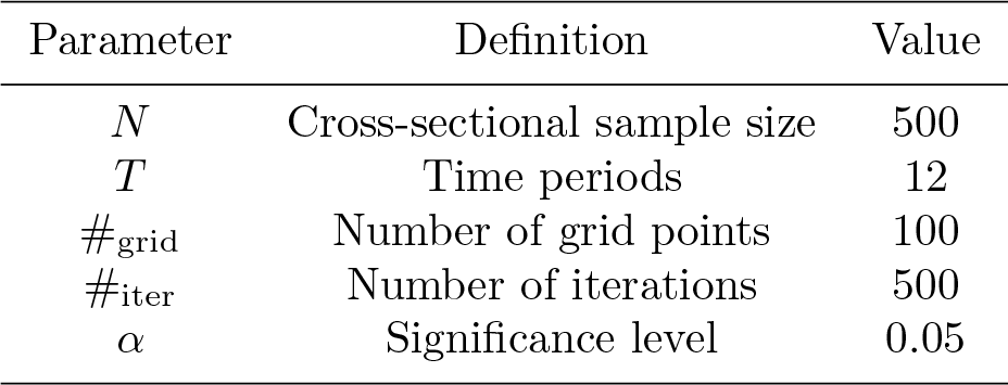
Moreover, x_i,t and ε_i,t were drawn independently from the centered normal distribution with a standard deviation of 1 and 0.25, respectively. For each iteration, we calculate the bootstrapped supW^∗ once following, for example, Giacomini, Politis, and White (2013). Consequently, we obtain 500 simulated supW and supW^∗ statistics. With these, we compute the bootstrap critical value, which is the empirical (1 − α) 100-percentile of those 500 supW^∗ statistics, and the rejection probability for the given α, which is the proportion of 500 supW statistics bigger than the bootstrap critical value.

4.1 Test size

Here we impose (β ₁ , β ₂ , δ ₀ , δ ₁ , δ ₂) = (0.5, 0.8, 0.0, 0.0, 0.0) so that H ₀ : δ = 0 holds. This implies the true underlying model is linear. The simulated rejection probability was 0.066, which is reasonably close to the true α = 0.05. Empirical distributions of supW and supW^∗ are as follows:

Figure 1.

Original and bootstrapped sup-Wald statistics under H₀.

4.2 Test power

Here we tested three sets of coefficient choices, maintaining H₁ : δ ≠ 0 holds:

Parameters	Values	Rejection probability
(β₁, β₂, δ₀, δ₁, δ₂)	(0.5, 0.8, 0.0, −0.5, 0.0)	1.00
	(0.5, 0.0, 0.0, −0.5, 0.0)	0.54
	(0.5, 0.0, 0.0, −0.9, 0.0)	0.96

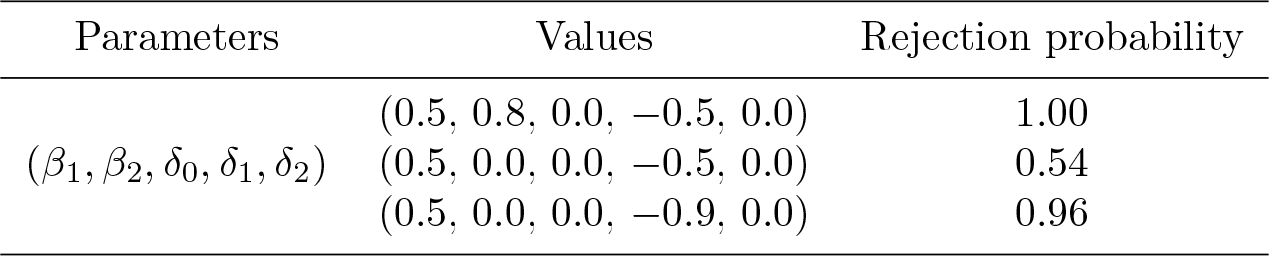
We observe that our test has significant power to reject H ₀ when H ₁ is true, especially when the true δ is sufficiently far from zero.

5 Application

We apply our method to evaluate the effect of obesity on work hours. Obesity is measured with body mass index (BMI), which is someone’s weight in kilograms divided by height in meters squared. Individuals with a BMI between 25 and 30 are considered to be overweight, and individuals with a BMI of 30 or higher are considered to be obese. Using data from the British Cohort Study, which can be accessed through the UK Data Service,² and the methods described in the earlier section, we examine how BMI is associated with work hours. For more detailed discussion, see Kim (2019).

In this example, we consider work hours and BMI of male workers using the following model with a kink in BMI:

y_{i t} = β_{0} + x_{i t} β_{1} + q_{i t} β_{2} + δ (q_{i t} - γ) 1 {q_{i t} \geq γ} + α_{i} + ε_{i t}

We present work hours as y_it for an individual i for a period t, x_it as family size, and q_it as BMI. We have two-period panel data (t = 1, 2) and take the first difference as follows to remove α_i, the individual time-invariant characteristics that are associated with work hours:

Δ y_{i}_{2} = Δ x_{i}_{2} β_{1} + Δ q_{i}_{2} β_{2} + δ (q_{i}_{2} - γ) 1 {q_{i}_{2} \geq γ} - (q_{i}_{1} - γ) δ 1 {q_{i}_{1} \geq γ} + Δ ε_{i}_{2}

To implement GMM estimation, we use instrumental variables birthweight (bweight), a worker’s own childhood BMI (bmic), and that worker’s parents’ BMIs (bmim, bmid) for BMI variables of Δq_i ₂ , q_i ₂ , q_i ₁ in the first-differenced model.

After loading the data, we first need to declare that the data are panel. The default model for xthenreg is a dynamic model. Because we consider a static model, not a dynamic model, we use the static option. We also impose a kink in the model by using the kink option:

The information preceding the table is as follows: N is the total number of unique subjects, T is the number of time periods, and the Number of moment conditions is provided based on the choice of instruments.

Because we change the set of included and excluded instruments using the inst() option, the number of moment conditions varies accordingly.

We can fit the model with a restriction on the sample:

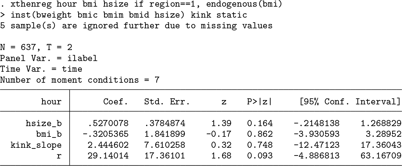
Next, we consider discontinuity in BMI effect without imposing a kink in the model.

y_{i t} = β_{0} + x_{i t} β_{1} + q_{i t} β_{2} + (δ_{0} + x_{i t} δ_{1} + q_{i t} δ_{2}) 1 {q_{i t} > γ} + α_{i} + ε_{i t}

By taking the first difference, we obtain the following model and fit it only with the static option.

Δ y_{i}_{2} = Δ x_{i}_{2} β_{1} + Δ q_{i}_{2} β_{2} + (δ_{0} + x_{i}_{2} δ_{1} + q_{i}_{2} δ_{2}) 1 {q_{i}_{2} > γ} - (δ_{0} + x_{i}_{1} δ_{1} + q_{i}_{1} δ_{2}) 1 {q_{i}_{1} > γ} + Δ ε_{i}_{2}

6 Conclusion

In this article, we presented a set of algorithms to facilitate inference for the dynamic threshold panel model with two regimes. An interesting future research avenue is to develop an algorithm to determine the number of regimes. The commonly used sequential approach in, for example, Bai and Perron (1998), where the linearity test is applied to each subsample until the test cannot reject the linearity null, is less appealing for the first-differenced GMM estimation because of the lack of the oracle property in the threshold estimate. The penalized approaches in Lee, Seo, and Shin (2016) or Lee et al. (2018) may prove useful.

8 Programs and supplemental materials

Supplemental Material, st0573 - Estimation of dynamic panel threshold model using Stata

Supplemental Material, st0573 for Estimation of dynamic panel threshold model using Stata by Myung Hwan Seo, Sueyoul Kim and Young-Joo Kim in The Stata Journal

Footnotes

7 Acknowledgments

This work was supported by the Ministry of Education of the Republic of Korea and the National Research Foundation of Korea (NRF-2017S1A5A8019707) and 2018 Hongik University Research Fund. Seo acknowledges financial support from the Center for National Competitiveness in the Institute of Economic Research.

8 Programs and supplemental materials

To install a snapshot of the corresponding software files as they existed at the time of publication of this article, type

Notes

References

Adam

C. S.

Bevan

D. L.

2005. Fiscal deficits and growth in developing countries. Journal of Public Economics 89: 571–597.

Bai

Perron

1998. Estimating and testing linear models with multiple structural changes. Econometrica 66: 47–78.

Giacomini

Politis

D. N.

White

2013. A warp-speed method for conducting Monte Carlo experiments involving bootstrap estimators. Econometric Theory 29: 567–589.

Hansen

B. E.

1999. Threshold effects in non-dynamic panels: Estimation, testing, and inference. Journal of Econometrics 93: 345–368.

Hidalgo

Lee

Seo

M. H.

2019. Robust inference for threshold regression models. Journal of Econometrics 210: 291–309.

Khan

M. S.

Ssnhadji

A. S.

2001. Threshold effects in the relationship between inflation and growth. IMF Staff Papers 48: 1–21.

Kim

Y.-J.

2019. The effect of weight on work hours. Unpublished manuscript.

Lee

Liao

Seo

M. H.

Shin

2018. Oracle estimation of a change point in high-dimensional quantile regression. Journal of the American Statistical Association 113: 1184–1194.

Lee

Seo

M. H.

Shin

2016. The lasso for high dimensional regression with a possible change point. Journal of the Royal Statistical Society, Series B 78: 193–210.

10.

Seo

M. H.

Shin

2016. Dynamic panels with threshold effect and endogeneity. Journal of Econometrics 195: 169–186.

11.

Wang

2015. Fixed-effect panel threshold model using Stata. Stata Journal 15: 121–134.

12.

Zhang

Zhou

Jiang

2017. Panel kink regression with an unknown thresh-old. Economics Letters 157: 116–121.

Supplementary Material

Please find the following supplemental material available below.

For Open Access articles published under a Creative Commons License, all supplemental material carries the same license as the article it is associated with.

For non-Open Access articles published, all supplemental material carries a non-exclusive license, and permission requests for re-use of supplemental material or any part of supplemental material shall be sent directly to the copyright owner as specified in the copyright notice associated with the article.

0.00 MB