distcomp: Comparing distributions

Abstract

In this article, I introduce the distcomp command, which assesses whether two distributions differ at each possible value while controlling the probability of any false positive, even in finite samples. I discuss syntax and the underlying methodology (from Goldman and Kaplan [2018, Journal of Econometrics 206: 143–166]). Multiple examples illustrate the distcomp command, including revisiting the experimental data of Gneezy and List (2006, Econometrica 74: 1365–1384) and the regression discontinuity design of Cattaneo, Frandsen, and Titiunik (2015, Journal of Causal Inference 3: 1–24).

1 Introduction

The new distcomp command implements a new statistical procedure for comparing distributions that was introduced in Goldman and Kaplan (2018). The usage is similar to a two-sample t test or two-sample Kolmogorov–Smirnov (KS) test, that is, ttest or ksmirnov(respectively) with the by() option (see [R] ttest or [R] ksmirnov). However, instead of comparing only the distributions’ means (like ttest) or testing only a single hypothesis of distributional equality (like ksmirnov), distcomp assesses equality of the distribution functions point by point. Thus, instead of a single rejection or nonrejection, distcomp displays ranges of values in which the distributions’ difference is statistically significant. It can also show goodness-of-fit (GOF) test results like those from ksmirnov.

The new procedure controls false positives with strong control of the familywise error rate (FWER), which is described later. As a special case, if the distributions are truly identical, then no ranges will be deemed statistically significant 95% of the time if a 5% level is used. This FWER is controlled in finite samples (not just asymptotically).

Even for GOF testing, distcomp may be preferred to ksmirnov because the new method’s sensitivity to deviations is more evenly spread across the distribution. This new GOF test was proposed by Goldman and Kaplan (2018), refining an idea from Buja and Rolke (2006). Specifically, the KS test has long been known to lack sensitivity to deviations in the tails of a distribution (for example, Eicker [1979, 117]). For example, if one sample has observed values 0.02, 0.04,…, 0.98, like a standard uniform distribution, the second sample may have even 6 out of 21 values exceeding 1,000,000 without a two-sided KS test rejecting at a 10% level. In contrast, distcomp rejects equality at even a 1% level. The following code shows such a result:

Section 2 discusses the methodology at a relatively intuitive level. Section 3 describes the syntax and usage of distcomp. Section 4 provides empirical examples that can be replicated with the provided do-file. Section 5 shows some of the theoretical foundations before section 6 concludes. If you are interested in related methods (onesided, one-sample, or uniform confidence bands), see Goldman and Kaplan (2018) and the corresponding R code. I use abbreviations for the cumulative distribution function (CDF), GOF, KS, and FWER.

2 A gentle introduction to methodology

This section discusses methodology at a relatively nontechnical level (compared with section 5). Interest is in the distribution of some outcome variable (like wage) for two groups (like union members and nonmembers). More specifically, the question is whether and where the two CDFs are different. Let F (·) be the first group’s CDF (like the CDF of wage for union members) and G(·) be the second group’s CDF. Estimated CDFs $\widehat{F}(·)$ and $\widehat{G}(·)$ are computed from i.i.d. samples. These are the stair-step functions like in the graphs in section 4.

Consider the KS GOF test. The null hypothesis is

$(\text{GOF})H_0:F(r) =G(r)\text{ for all }r$

1

identical CDFs. If H ₀ is true, then $\widehat{F}(·)$ and $\widehat{G}(·)$ should be “close” to each other; if not, the test rejects.

KS defines “close” with vertical distance. At point r, this distance is

$\widehat{D}(r)\equiv |\widehat{F}(r)-\widehat{G}(r)|$

To compare the entire functions, KS looks across all r to find the biggest gap, max_r $\widehat{D}(r)$ .Fortunately, under H ₀, the sampling distribution of the “biggest gap” does not depend on the true distribution, so it can be simulated. Thus, finite-sample p-values can be simulated without any asymptotic approximation, and the KS test can control the type I error rate at level α.

Instead of (1), null hypotheses can be defined to show where two distributions differ. For each possible value r of the outcome variable, define

$H_0{ }_{\text{r}}:F(r) =G(r)$

2

The GOF null hypothesis could be rewritten as

$(\text{GOF again})H_0:\text{ all }{H}_0{ }_{\text{r}}\text{ are true}$

Whereas the GOF test distinguishes only whether all H _{0 r} are true or at least one is false, now we care about specifically which H _{0 r} are true and which are false. This is summarized by distcomp with the ranges of r for which H _{0 r} is rejected.

It does not work to run a level α t test on all H _{0 r}. Imagine just two values, r = 1, 2 and α = 0.1 = 10%. Let both H _{0 r} be true. Then, each test’s probability of not rejecting is 0.9. Assuming independence for simplicity, the probability that neither rejects is (0.9)(0.9) = 0.81, so the probability that one or both rejects is 1−0.81 = 0.19. That is, the probability of at least one type I error (false positive) is 19%, which is much larger than the desired α = 10%. This is called the “multiple testing problem”.

The following is one way to define a type I error control for multiple testing. A “familywise error” is made if at least one true H _{0 r} is rejected. For example, if H _{0 r} is true only for r ≤ 0, then a familywise error occurs if any H _{0 r} with r ≤ 0 is rejected. The probability of such an error is the FWER:

FWER ≡ Pr(reject any true H _{0 r} )

“Weak control of FWER at level α” guarantees FWER ≤ α when all H _{0 r} are true. The distcomp methodology achieves “strong control” of FWER, meaning FWER ≤ α regardless of which H _{0 r} are true. Put differently, with strong control of FWER at a 10% level, there will be zero false positives 90% of the time.

One way to test (2) and achieve strong control of FWER is to extend the KS approach. Specifically, imagine that c is the simulated critical value given n and α. It seems natural to reject H _{0 r} when $\widehat{D}(r)>c$ .

The weak control of FWER comes from the KS GOF test’s properties. When the GOF H ₀ is true (so all H _{0 r} are true), the probability of GOF rejection is α: $\text{Pr}({\text{max}}_{\text{r}}\widehat{D}(r)>c) =\alpha$ . Because max_r $\widehat{D}(r)> c$ is equivalent to “at least one H _{0 r} is rejected”, the probability of rejecting at least one H _{0 r} (that is, FWER) is also α.

The KS approach also has strong control of FWER. The intuition is that when all H _{0 r} are true (as with weak control of FWER), the opportunity for a familywise error is greatest, so FWER is highest. If fewer H _{0 r} are true, then there is less opportunity for a familywise error. In the extreme, when no H _{0 r} is true, it is impossible to make a familywise error. This intuition is proven correct for a certain class of methods including the KS approach and distcomp, although it can fail in other cases.

The KS approach controls FWER, but it distributes power unevenly. This means it detects certain types of differences between F (·) and G(·) very well but detects others very poorly. Unless we know what type of difference to expect, it seems prudent to desire power against all differences. distcomp achieves this without sacrificing the finite-sample strong control of FWER.

One shortcoming of KS is its implicit symmetry. The definition of $\widehat{D}(r)$ has an absolute value; positive and negative values are treated the same. This makes sense with normal distributions, but normality is only an asymptotic approximation. The finite-sample distribution of $\widehat{F}(r)$ is actually binomial, which is especially skewed (not symmetric) when r is in the tails.

KS also ignores scale differences. The variance of $\widehat{F}(r)$ is highest when r is the median and nears zero when r is in the tails. The variance of $\widehat{D}(r)$ similarly varies with r. Even if $\widehat{D}(r)$ were normal, it would be much more likely to have a large value with median r than with r in the tails, where H _{0 r} is very unlikely to be rejected.

By using the finite-sample sampling distributions of $\widehat{F}(r)$ and $\widehat{D}(r)$ , distcomp accounts for both skewness and scale differences across r, unlike KS.

3 The distcomp command

The distcomp command compares two distributions. One variable in the data (varname below) is the variable for comparison like price or income. Another variable (groupvar below) takes only two distinct values, defining two groups like an indicator or dummy for male whose value is 0 or 1 or a state abbreviation whose value is NY or CA.

The validity of two assumptions should be considered in practice. First, sampling is assumed independent and identically distributed (i.i.d.) from the two respective group population distributions, and it is assumed the groups are sampled independently. Second, the variable of interest (varname) is assumed to have a continuous distribution, but some amount of discreteness is okay. In particular, if there are duplicate values within each sample, but no “ties” (same value observed in both samples), then the properties remain the same. However, if there are many ties, then the theoretical results do not apply directly, and the properties may change substantially. In the absence of theoretical results allowing ties, simulations suggest the method may become conservative, controlling the FWER at a level even lower than the level specified. One such simulation is included in the accompanying distcomp_examples.do file, in which the nominal FWER is 10%, but the simulated FWER is near 0%.

distcomp displays results for the global (GOF) test first. This is the same type of test as the (two-sample) KS test. That is, the null hypothesis is that the two CDFs are identical. This could be false even if the two distributions’ means are identical (and ttest does not reject), for example, with normal distributions with the same mean but different standard deviation. The global test results are always reported for levels 1%, 5%, and 10%. Optionally, a p-value is also reported; it must be simulated and can substantially increase computation time with large sample sizes. ¹ The test is generally more powerful than KS. The GOF methodology was proposed by Goldman and Kaplan (2018) to refine an idea from Buja and Rolke (2006).

The second results displayed are for a multiple testing procedure. They show ranges of values for which the difference between CDFs is statistically significant, accounting for the multiple testing nature of the procedure (that is, many different points are tested simultaneously). Instead of a single, GOF null hypothesis, there is a set of many null hypotheses. Within the set, each individual hypothesis specifies equality of the two CDFs at a different point. That is, if F (·) and G(·) are the two CDFs, then each individual null hypothesis is H _{0 x} : F (x) = G(x), and the set of such hypotheses for all possible values of x is considered. The multiple testing procedure rejects equality at certain values of x while controlling the probability of any type I error (false positive). The probability of any false positive is known as the FWER. The distcomp procedure controls the finite-sample (not just asymptotic) FWER at the desired level specified by the user. The output shows the ranges of x where H _{0 x} : F (x) = G(x) is rejected. This methodology is from Goldman and Kaplan (2018).

By default, a plot is generated with the empirical CDFs of the two groups, along with the rejected ranges (if any).

The restriction of FWER levels to 1%, 5%, and 10% allows nearly instantaneous computation (when a p-value is not requested). The reason is that a table of precise “critical values” for these specific levels has been simulated ahead of time. In small samples, as with the KS test, it is often impossible to attain exactly 1%, 5%, or 10%. For example, for certain sample sizes, it may be possible only to have FWER of 9.6% or 10.6%, but nothing in between. To make this transparent, the exact finite-sample FWER level has also been presimulated and is returned by distcomp. In some cases, an analytic formula (based on simulations) is used, in which case the presimulated exact FWER is not available. Except with very small samples, the practical difference between specified and actual FWER level is usually negligible.

3.1 Syntax

distcomp varname [i]f [in] , by( groupvar ) [ alpha(# ) pvalue noplot] by is allowed; see [U] 11.1.10 Prefix commands.

3.2 Options

by( groupvar ) specifies a binary variable that identifies the two groups whose distributions are compared. by() is required. The variable does not need to have values 0 and 1 specifically; any two values are fine, like 1 and 5 or cat and dog.

alpha( # ) specifies the FWER level at #. The default is alpha(0.10), that is, a 10% probability of any false positive. Other accepted values are 0.05 and 0.01 (meaning 5% and 1%).

pvalue requests the global p-value be simulated. The computation time depends on the sample size. For prohibitively large samples, the global test’s rejections at levels 1%, 5%, and 10% (which do not require simulation) can be used to roughly approximate the p-value. For example, if only the 10% test rejects, then 0.05 < p < 0.10.

noplot suppresses the plot.

3.3 Stored results

distcomp stores the following in r():

Scalars

Matrices

4 Examples

The examples in this section can all be replicated with the file distcomp_examples.do. Some code is omitted here to conserve space.

4.1 Simple example with built-in dataset

The following example compares the hourly wage distributions of union and nonunion workers in the U.S. National Longitudinal Study of Young Women dataset shipped with Stata, with a 10% statistical significance level.

Three main results are displayed. The first result says that the global/GOF null hypothesis that the two wage distributions are identical is rejected at a 1% (and thus 5% and 10%) level. The statistical significance is even greater because the p-value is even lower than 0.01. There is strong evidence that union and nonunion wage distributions are not identical. The second result shows the range of wage values at which CDF equality is rejected while controlling the FWER at 10%. In this example, the range covers most of the wage distribution from around the 2nd percentile ($2.38/hr) to almost the 86th percentile ($11.61/hr). This suggests a restricted first-order stochastic dominance relationship as defined in condition I of Atkinson (1987, 751). The empirical CDF graph (figure 1) illustrates this result too.

Figure 1.

Empirical CDFs from the U.S. National Longitudinal Study of Young Women data

Figure 1 shows the default plot generated by distcomp. It shows the empirical CDFs for union wage and nonunion wage. These are step functions, but each step is very small because the sample size is moderate (461 union, 1,417 nonunion). The thick horizontal line near the bottom shows the ranges where CDF equality was rejected (10% FWER level). It is clear that union wages tend to be higher in the sample (hence the union CDF lies below the nonunion CDF). However, the empirical CDFs alone cannot show statistical significance. The line at the bottom shows that this difference is indeed statistically significant at a 10% FWER level across most of the distribution, though not the upper tail.

Union and nonunion wages can be compared for certain subgroups by using an if qualifier or by prefix. For example, the above analysis can be repeated for each different race group by typing by race, sort: distcomp wage, by(union) p or for only married individuals by typing distcomp wage if married==1, by(union) p.

4.2 Example with simulated data

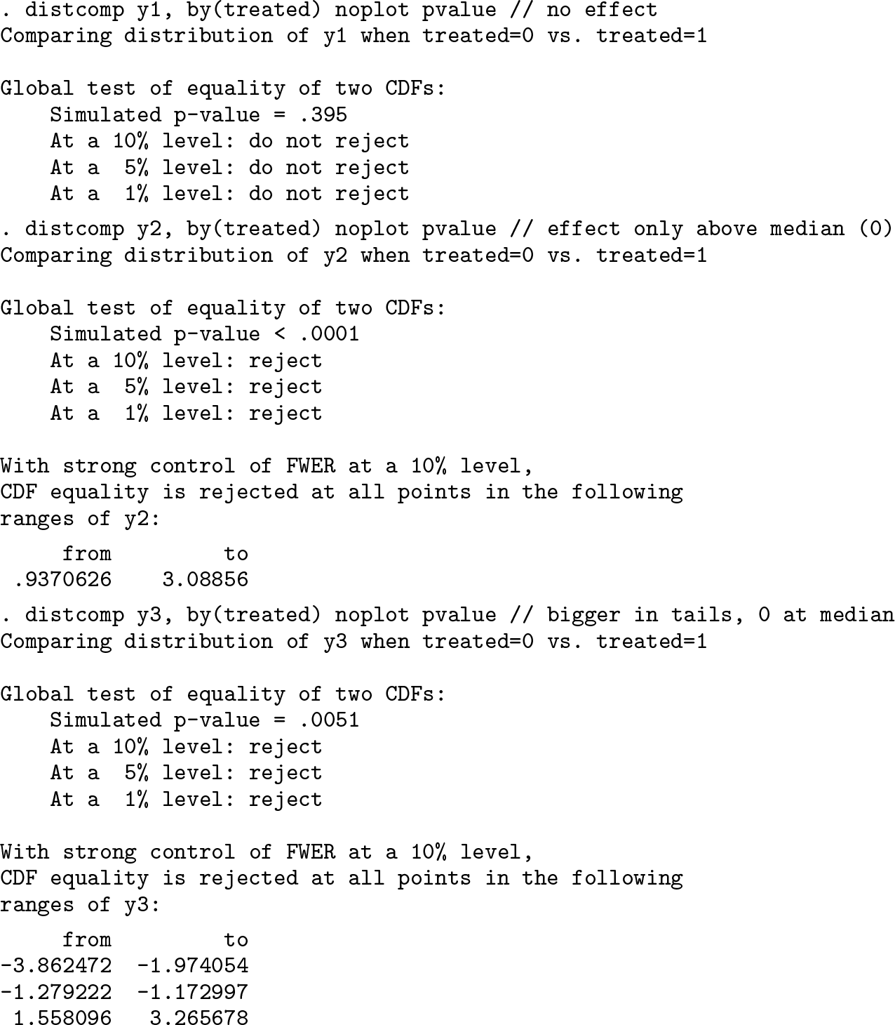
The following example uses simulated data. The code (including the random seed) to replicate the simulated data is in distcomp_examples.do but omitted here. The control group sample has 50 observations drawn independently from a standard normal distribution. The first treatment group also has 50 observations drawn independently from a standard normal distribution; that is, the treatment and control population distributions are identical (but sample values differ). The second treatment group is the same for below-median individuals, but the treatment increases the outcome by two units for individuals with above-median values. The third treatment has no effect on the mean, but it affects the spread; values are drawn from a mean-zero normal distribution with a standard deviation of three.

Running distcomp produces the following results:

Above, for the y1 case, where the control and treatment distributions are equal, nothing is statistically significant at conventional levels. The distcomp GOF test does not reject equality even at a 10% level (the GOF p-value is 0.395), so no ranges are rejected at a 10% FWER level. The empirical CDFs differ, but distcomp says these differences are not statistically significant at a 10% level.

For the y2 case, where the treatment has an effect, but only above the median (which is zero), the distcomp results reflect this. First, equality of the distributions is rejected at a level well below 1% (p < 0.0001). Then, more specifically, distcomp says equality is rejected over the range [0.937, 3.089]. The distributions indeed differ over this range. They actually differ over the larger range from zero to infinity, but there is not enough data to be certain that differences closer to zero are statistically significant. The same applies for differences far in the upper tail (above 3.089).

For the y3 case, where the treatment affects the standard deviation, the true CDFs differ everywhere except at zero, and again distcomp reflects this. In addition to rejecting global equality at a 1% level, distcomp identifies three specific ranges of values (that exclude zero) where the distributions differ. Similarly to the second case, it is most difficult to infer a difference near zero (where the CDFs are actually equal) and far in the tails (where there are few or no observations). Given the same FWER level, more data would be required to enlarge the ranges where we are statistically confident in a CDF difference.

4.3 Example with experimental data

The following example uses data from Gneezy and List (2006) to test for distributional treatment effects. A longer version appears in Goldman and Kaplan (2018, §8.1). In brief, Gneezy and List (2006) paid control-group individuals an advertised hourly wage and treatment-group individuals an unexpectedly larger “gift” wage upon arrival. The “gift exchange” question from behavioral economics is whether the higher wage induces higher effort in return. The experiment is run separately for library data entry and doorto-door fundraising tasks. The sample sizes are small: 10 and 9 for control and treatment (respectively) for the library task and 10 and 13 for fundraising. With small samples, the finite-sample FWER control of distcomp is especially desirable. Complementing the original results of Gneezy and List (2006), Goldman and Kaplan (2018) examine heterogeneity in the treatment effect during the first few hours of work with results seen below.

For the library task, although the sample values look different, the sample sizes are too small for the differences to be statistically significant at a 5% FWER level (twosided). The FWER level would have to be 14.1% (the GOF p-value) before rejecting equality in any range.

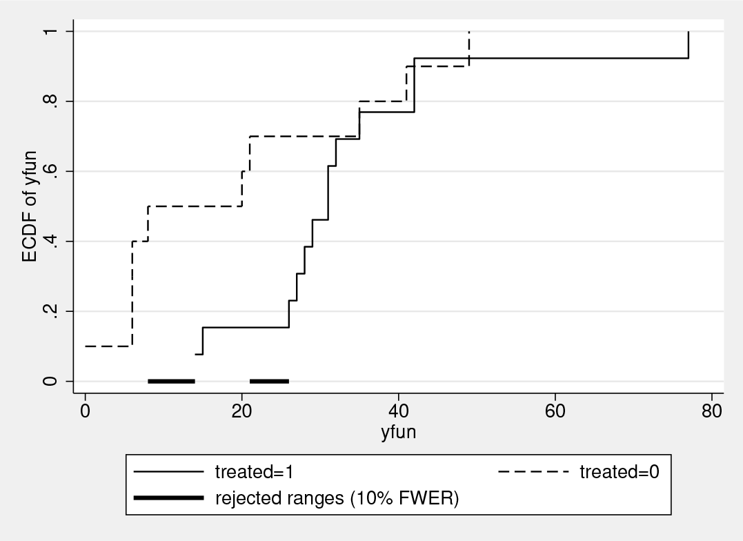
For the fundraising task, even though the sample sizes are again small, the treatment effect is statistically significant at a 5% level (two-sided). The p-value is 0.040 for CDF equality. More specifically, distcomp identifies the range of $8–$14 as statistically significant at a 5% FWER level. ² This range is near the bottom of the distribution. Opposite the library data entry task, where the gift wage treatment seemed to have the biggest effect on the upper end of the productivity distribution, the gift wage seems to have the biggest effect on the bottom end of the productivity distribution for door-todoor fundraising.

Figures 2 and 3 show the fundraising and library data entry empirical CDFs, respectively. These are again the graphs generated automatically by distcomp. These graphs show the direction of the gift wage effect (higher productivity), but without distcomp it is unclear where the differences are statistically significant.

Figure 2.

Empirical CDFs from experiment (fundraising)

Figure 3.

Empirical CDFs from experiment (library data entry)

4.4 Example with regression discontinuity

The following regression discontinuity example uses data from Cattaneo, Frandsen, and Titiunik (2015). A longer version (with results from R code) appears in Goldman and Kaplan (2018, §8.2). In brief, the research question is about the benefit of incumbency in U.S. Senate elections. The regression discontinuity idea is essentially to consider elections where the incumbent won the prior election by a very small margin. Cattaneo, Frandsen, and Titiunik (2015) discuss a balance test-based bandwidth selection that suggests h=0.75 percentage points is a small enough margin of victory that the outcome is (almost) as good as randomized.

In the following code and results, demmv is the Democratic margin of victory in the previous election for some Senate seat (in percentage points), which is negative if the Republican won. Thus, the incumbent is a Democrat if demmv exceeds the threshold R0=0. Also, demvoteshfor2 is the Democratic vote share in the current election for the same Senate seat. Below, the distribution of Democratic vote share when the incumbent is a Democrat is compared with when the incumbent is a Republican, restricted to cases where the incumbent’s election was determined by a margin of victory of 0.75 points or less.

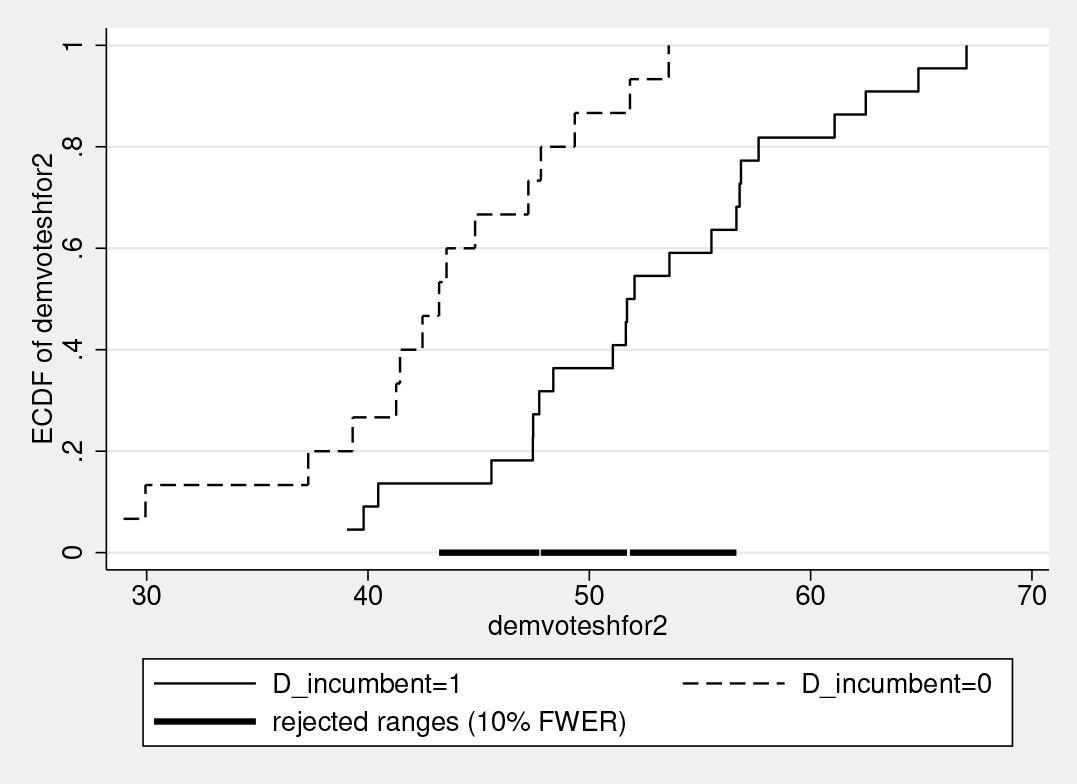
The results show the incumbency effect to be statistically significant across most of the distribution. With only two slim gaps, equality of the vote share distributions is rejected over the range from 43.2% to 56.6% of the vote. Of course, beyond statistical significance, it is also important to estimate the magnitude of the incumbency effect by the usual regression discontinuity estimator. Figure 4 shows that in the sample, the vote share distribution for incumbents (who had a very small margin of victory) first-order stochastically dominates the distribution for challengers (that is, nonincumbents). It looks like with a larger sample size, equality could be rejected over an even larger range. The graph also gives a sense of the magnitude of the incumbency effect.

Figure 4.

Empirical CDFs from regression discontinuity design

5 Methods and formulas

This section contains additional theoretical details from Goldman and Kaplan (2018). It may provide a deeper understanding for some readers, although it may also be skipped without hindering successful application of distcomp in practice.

Notationally, let F _X(·) be the population CDF for the first group, and let F _Y (·) be the population CDF for the second group. The GOF null hypothesis is $H_0:F_{\text{X}}(·) =F_{\text{Y}}(·)$ ; that is, $F_{\text{X}}(r) =F_{\text{Y}}(r)$ for all real numbers r. The distcomp command also considers the individual hypotheses $H_{0\text{r}}:F_{\text{X}}(r) =F_{\text{Y}}(r)$ .

For more formal discussion, the following notation and definitions are helpful. These are adapted from the section on multiple testing by Lehmann and Romano (2005, §9.1). For the family of null hypotheses H _{0 r} indexed by real numbers r, let T ≡ {r : H _{0 r} is true}, the set of values of r for which hypothesis H _{0 r} is true. The FWER is the probability of falsely rejecting at least one true hypothesis:

FWER ≡ Pr (reject any H _{0 r} with r ∊ T )

“Weak control” of FWER at level α requires FWER ≤ α if each H _{0 r} is true, that is, if the GOF null hypothesis $H_0:F_{\text{X}}(·) =F_{\text{Y}}(·)$ is true, but it allows FWER > α if some H _{0 r} are false. In this setting, weak control of FWER is equivalent to size control for the corresponding GOF test that rejects $H_0:F_{\text{X}}(·) =F_{\text{Y}}(·)$ when at least one H _{0 r} is rejected. “Strong control” of FWER requires FWER ≤ α for any T , that is, for any two CDFs F _X(·) and F _Y (·). Strong control implies weak control, but not vice versa.

Strong control of FWER, even in small samples, is achieved by distcomp. The “rejected ranges” displayed by distcomp are the values of r for which H _{0 r} is rejected when strongly controlling the FWER at the specified level α.

The two most important properties of distcomp are its strong control of finitesample FWER and its improved sensitivity to tail differences compared with ksmirnov. I now describe the procedure mathematically, and then further discuss achievement of these two properties.

Steps for computation of distcomp are given in method 5 of Goldman and Kaplan (2018). The idea is to compute a uniform confidence band (detailed below) for each unknown CDF and then reject H _{0 r} for any r where the bands do not overlap. Notationally, let $B_{k,n}^{{ }^{\tilde{\alpha }}}$ denote the $\tilde{\alpha }$ -quantile of the Beta $(k, n+\text{ 1}-k)$ distribution, defining $B_{k,n}^{{ }^{\tilde{\alpha }}}=0$ and $B_{n+1,n}^{{ }^{\tilde{\alpha }}}=1$ for any $\tilde{\alpha }$ , and denote sample sizes as n _X and n _Y. The uniform confidence bands for F _X(·) and F _Y (·) are, respectively, $[{\widehat{\mathcal{l}}}_{\text{X}}(·), {\widehat{u}}_{\text{X}}(·)]$ and $[{\widehat{\mathcal{l}}}_{\text{Y}}(·), {\widehat{u}}_{\text{Y}}(·)]$ , where for some $\tilde{\alpha }$ , ${\widehat{\mathcal{l}}}_{\text{X}}(r) =B_{n_X{\widehat{F}}_X\left(r\right),n_X}^{\tilde{\alpha }}$ , ${\widehat{u}}_{\text{X}}(r) =B_{n_X{\widehat{F}}_X\left(r\right),n_X}^{1-\tilde{\alpha }}$ and similarly replacing X with Y. Then, H _{0 r} is rejected when either ${\widehat{\mathcal{l}}}_{\text{X}}(r)> {\widehat{u}}_{\text{Y}}(r)$ or ${\widehat{\mathcal{l}}}_Y(r)> {\widehat{u}}_X(r)$ The value of $\tilde{\alpha }$ is the largest value such that the probability of rejecting any H _{0 r} (that is, the FWER) does not exceed α when $X_i\stackrel{\text{i}.\text{i}.\text{d}}{~}$ . Unif(0, 1), i = 1,…, n _X, and $Y_i\stackrel{\text{i}.\text{i}.\text{d}}{~}$ . Unif(0, 1), i = 1,…, n _Y , which is determined by simulation.

Although $\tilde{\alpha }$ is chosen to guarantee FWER control only when both F _X(·) and F _Y (·) are standard uniform CDFs, this extends to any $F_X(·) =F_Y(·)$ . The key insight is that at a given r, after one determines $\tilde{\alpha }$ (and n _X and n _Y ), rejection of H _{0 r} depends only on ${\widehat{F}}_X(r)$ and ${\widehat{F}}_Y(r)$ , which are step functions that increase only at observed sample values. That is, rejection of H _{0 r} depends only on the number of X _i below r and the number of Y _i below r, which yield ${\widehat{F}}_X(r)$ and ${\widehat{F}}_Y(r)$ when divided by n _X and n _Y , respectively. Consequently, whether any H _{0 r} is rejected depends only on the relative order of observed X _i and Y _i values, not on the values themselves. This implies that applying any monotonic transformation to the data does not affect the FWER. When $F_X(·) =F_Y(·) =F(·)$ , we could sample X _i and Y _i from F by first drawing standard uniform random variables and then applying $F^{-\text{1}}(·)$ . But because $F^{-\text{1}}(·)$ is a monotonic transformation, it will not affect FWER, so any F (·) will produce identical FWER as when X _i and Y _i are simply standard uniform themselves.

The above argument concerns only weak control of FWER; the extension to strong control is not obvious. Indeed, one of the contributions of Goldman and Kaplan (2018) is their Lemma 2, which proves weak control implies strong control for any procedure where rejection of H _{0 r} depends only on ${\widehat{F}}_X(r)\text{ and}\hspace{0.17em}{\widehat{F}}_{\text{Y}}(r)$ , which is the case here. The intuition is that if FWER is controlled when $F_{\text{X}}(r) =F_{\text{Y}}(r)$ for all r, then changing F _X(·) so that $F_{\text{X}}(r)\ne F_{\text{Y}}(r)$ at some r does not somehow increase the probability of rejecting the remaining H _{0 r} where $F_{\text{X}}(r) =F_{\text{Y}}(r)$ .

Computationally, the difficult part of the procedure is determining $\tilde{\alpha }$ . Because $\tilde{\alpha }$ depends only on α, n _X, and n _Y , a large table of precise values was simulated ahead of time for the most common levels of α = 0.01, 0.05, 0.10 and included in distcomp. This enables nearly instantaneous computation of distcomp.

For the second important property of improved tail sensitivity, it is insightful to look at the uniform confidence bands more closely. Here we look at a single sample of X _i with CDF F (·). A “uniform confidence band” for F (·) consists of an upper function $\widehat{u}(·)$ and lower function $\widehat{\mathcal{l}}(·)$ that may depend on the data and satisfy $\text{Pr}\{\widehat{\mathcal{l}}(·)\le F(·)\le \widehat{u}(·)\}\ge \text{1}-\alpha$ for confidence level (1 − α) × 100%, where $\widehat{\mathcal{l}}(·)\le F(·)\le \widehat{u}(·)$ means $\widehat{\mathcal{l}}(r)\le F(r)\le \widehat{u}(r)$ for all r. Such a band may be constructed by inverting the onesample KS test, but its pointwise coverage probability varies greatly with r. That is, $\text{Pr}\{\widehat{\mathcal{l}}(r)\le F(r)\le \widehat{u}(r)\}$ is much larger (closer to 100%) when r is in the tails of the true distribution (that is, when F (r) is nearer 0 or 1) than when r is in the middle (that is, F (r) nearer 0.5). In contrast, the pointwise coverage probability of the uniform confidence band used in distcomp is (nearly) the same for all values of r.

The even pointwise coverage probability property of the uniform confidence bands used by distcomp can be seen as follows. Similar points are made by Buja and Rolke (2006, top of page 28). Let X _{n : k} denote the kth order statistic in a sample of size n, that is, the kth smallest value in the sample, so $X_{\text{n}:\text{1}}<···< X_{\text{n}:\text{k}}<···< X_{\text{n}:\text{n}}.$ From Wilks (1962), $F(X_{\text{n}:\text{k}})~\text{Beta}(k, n+\text{ 1}-k)$ if F (·) is continuous. This follows from an application of the “probability integral transform”: $F\left(X_i\right)\stackrel{\text{i}.\text{i}.\text{d}}{~}$ . Unif(0, 1), and $F(X_{\text{n}:\text{k}})$ follows the same distribution as the kth order statistic from a sample of n standard uniform random variables, which is Beta $(k, n+\text{ 1}-k)$ . Thus, because $B_{k,n}^{\tilde{\alpha }}$ is defined as the αe-quantile of that same distribution, $\text{Pr}\{B_{k,n}^{\tilde{\alpha }}\le F(X_{\text{n}}{{ }_{:}}_{\text{k}})\le B{\text{k}}_{k,n}^{{{ }^{\text{1}}}^{-}{ }^{\tilde{\alpha }}}\}=\text{ 1}-\text{2}\tilde{\alpha }$ exactly, for any k and n, irrespective of F (·). In the earlier expressions, $[\widehat{\mathcal{l}}(·), \widehat{u}(·)]$ is essentially taking pointwise intervals $[\widehat{\mathcal{l}}(X_{\text{n}:\text{k}}), \widehat{u}(X_{\text{n}:\text{k}})\left] =\right[B_{{ }^{k,n}}^{\tilde{\alpha }}{B}_{{ }^{k,n}}^{\text{1}-\tilde{\alpha }}]$ and connecting them with a stair-step interpolation. This implies pointwise coverage probability of $\text{1}-\text{2}\tilde{\alpha }$ at every order statistic (and only somewhat larger at other points).

The $\text{1}-\text{2}\tilde{\alpha }$ probability at each order statistic contrasts the KS pointwise coverage probability that is much higher in the tails. This difference translates directly to the ability to detect deviations across different values: the KS sensitivity or power is concentrated in the center of the distribution, whereas distcomp spreads its power evenly across the whole distribution. Put differently, KS implicitly uses a much larger pointwise statistical significance level for testing H _{0 r} near the center of the distribution and much smaller significance level in the tails, whereas distcomp uses approximately the same level of statistical significance for all H _{0 r}.

6 Conclusion

In addition to a two-sample GOF test that improves upon the KS test, the distcomp command provides a detailed, point-by-point assessment of statistically significant differences between two distributions. This is much more informative than existing GOF tests (like the ksmirnov command) or t tests for mean equality (like ttest) while still controlling the false positive rate, with strong control of the FWER. Potential applications abound, such as descriptions of how a variable’s distribution changes over time or differs between groups (geographic, socioeconomic, etc.), regression discontinuity designs, and perhaps especially in program evaluation.

8 Programs and supplemental materials

Supplemental Material, st0579 - distcomp: Comparing distributions

Supplemental Material, st0579 for distcomp: Comparing distributions by David M. Kaplan in The Stata Journal