Sage Journals: Discover world-class research

Abstract

We introduce a command, fayherriot, that implements the Fay– Herriot model (Fay and Herriot, 1979, Journal of the American Statistical Association 74: 269–277), which is a small-area estimation technique (Rao and Molina, 2015, Small Area Estimation), in Stata. The Fay–Herriot model improves the precision of area-level direct estimates using area-level covariates. It belongs to the class of linear mixed models with normally distributed error terms. The fayherriot command encompasses options to a) produce out-of-sample predictions, b) adjust nonpositive random-effects variance estimates, and c) deal with the violation of model assumptions.

Keywords

st0570 fayherriot disaggregated indicators small-area estimation (log-transformed) Fay–Herriot model empirical best linear unbiased predictor

1 Introduction

Various national and international institutions, including the United Nations (Leadership Council of the Sustainable Development Solutions Network 2015) and the Organisation for Economic Co-operation and Development (Piacentini 2014), collect comprehensive indicator sets for monitoring purposes. Many indicators refer to subnational areas or domains: federal states, economic sectors, societal groups, etc.

In the socioeconomic context, domain-level indicators are usually derived from population surveys by direct estimation. Direct estimates are based only on the survey data, so small sample sizes can limit their precision. Thus, institutions that provide these indicators usually require a minimum number of observations per domain or impose limits on the variability of the estimates (Eurostat 2013; Tzavidis et al. 2018). Further more, direct estimates cannot be obtained for out-of-sample domains, that is, domains without any observation in the sample.

Small-area estimation techniques use auxiliary data from additional data sources to improve the precision of survey-based direct estimates. Two basic model types can be distinguished: unit- and area-level models. Unit-level models require survey and auxiliary data at the unit level, that is, individual- or household-level information in each domain. Examples are the model proposed by Battese, Harter, and Fuller (1988) and the empirical best predictor by Molina and Rao (2010). In comparison, area-level models, such as the Fay–Herriot (FH) model (1979),¹ require only domain-level auxiliary data, hence their popularity in applied research.

fayherriot provides empirical best linear unbiased predictors (EBLUP), which are linear combinations of the domain-level direct estimator and a regression-synthetic component based on a linear model. The underlying model can also be expressed as a special linear mixed model. In contrast to a standard linear mixed model [encompassed in mixed (Rabe-Hesketh and Skrondal 2012) or gllamm (see [R] gllamm)], the FH model builds on two error terms on the domain level, with domain-specific variances of one error term and a common variance of the other error term. The model assumes linearity and normality of its two error terms. Corral et al. (2018) implement a standard version.

fayherriot extends the existing possibilities in Stata and performs the following:

estimation of the FH model as described in Rao and Molina (2015, 123–129) with restricted maximum likelihood (REML) and maximum likelihood estimation (MLE) of the variance of the random effects,

estimation of the mean squared error (MSE) as proposed in Datta and Lahiri (2000) and Prasad and Rao (1990),

prediction and MSE estimation for out-of-sample domains (Rao and Molina 2015, 126 and 139),

estimation with adjusted methods as proposed in Li and Lahiri (2010) and Yoshimori and Lahiri (2014) to deal with nonpositive estimates of the variance of the random effects,

estimation of the log-transformed FH model including a bias correction by Slud and Maiti (2006) to deal with violations of model assumptions, for example, non normality of the error terms, and

estimation of the FH model for proportions defined on the [0, 1] interval, that is, with the dependent variable transformed by the arcsine square root transformation. The back-transformation and the corresponding boundaries of a bootstrap confidence interval following Casas-Cordero Valencia, Encina, and Lahiri (2016, 394–397) and Schmid et al. (2017, 1173–1177) are provided.

2 The FH model

2.1 Modeling

The FH model (Fay and Herriot 1979) combines domain-level direct estimates (based on survey data) with aggregated domain-level covariates (for example, from register or administrative data). The direct estimator should be a linear statistic such as an arithmetic mean, total, or share.

The FH model builds on a sampling and a linking model. According to the sampling model,

{\hat{θ}}_{d} = θ_{d} + e_{d} for d = 1, . . ., D

the observed direct estimator for domains $d = 1, . . ., D, {\hat{θ}}_{d}$ , is composed of the true value, θ_d , and a sampling error, e_d , with mean zero and variance $σ_{e_{d}}^{2}$ . The model assumes that the sampling error variance of each domain is known. In practice, the variance of the direct estimator is used frequently as an estimate for $σ_{e_{d}}^{2}$ (You and Chapman 2006). To consider sampling weights in the FH model, one can use the weighted direct estimator and its corresponding variance. For example, one can use the Horvitz–Thompson estimator for the mean (Horvitz and Thompson 1952). According to the linking model,

θ_{d} = x_{d}^{T} β + u_{d} for d = 1, . . ., D

the true value, θ_d , is explained by the domain-specific covariates, x _d ; a random effect, u_d ; and the regression parameters, β. The random effect is independently, identically, and normally distributed with mean zero and variance $σ_{u}^{2}$ . The model assumes interdomain correlations to be zero.

Combining the sampling and the linking models gives the FH model, which is a linear mixed model of the form

{\hat{θ}}_{d} = x_{d}^{⊤} β + u_{d} + e_{d} for d = 1, . . ., D

The FH estimator (EBLUP) is given by ${\hat{θ}}_{d}^{^{FH}} = x_{d}^{^{⊤}} \hat{β} + {\hat{u}}_{d}$ . It can also be expressed more intuitively as a weighted average of the direct and a regression-synthetic estimator,

{\hat{θ}}_{d}^{FH} = {\hat{γ}}_{d} {\hat{θ}}_{d} + (1 - {\hat{γ}}_{d}) x_{d}^{T} \hat{β}

The estimate ${\hat{γ}}_{d} = {\hat{σ}}_{u}^{2} / ({\hat{σ}}_{u}^{2} + σ_{e_{d}}^{2})$ , or the “shrinkage factor”, weights the direct estimate and the regression-synthetic part. The weight on the direct estimate decreases with the sampling error variance.

For out-of-sample domains, ${\hat{γ}}_{d}$ is not defined, and the regression-synthetic estimate $x_{d}^{T} \hat{β}$ is used. A domain is treated as out-of-sample if either the direct estimate or the sampling error variance is missing. Missing values in the domain-specific covariates (usually obtained from register or administrative data) are not allowed; that is, each explanatory variable needs to have a value for each domain.

2.2 Estimating the variance of the random error

The FH model requires an estimation of the variance of the random error, $σ_{u}^{2}$ , and of the regression parameters, β. Standard estimation techniques for $σ_{u}^{2}$ are, among others, REML and MLE. These methods do not guarantee positive variance estimates (Yoshimori and Lahiri 2014; Li and Lahiri 2010). Especially if there are few domains, the variance estimates can be negatively biased or even below zero. In the latter case, the variance estimate is set to zero. Underestimating the variance component could lead to a significant overshrinkage of the direct estimate to the regression-synthetic part; that is, too much weight is put on the regression-synthetic part.

Adjusted estimation methods, such as the adjusted maximum residual-likelihood approach (ARYL) following Yoshimori and Lahiri (2014) and the adjusted maximum-profile likelihood (AMPL) following Li and Lahiri (2010), ensure strictly positive variance estimates. fayherriot allows the estimation of $σ_{u}^{2}$ with REML (as the default), MLE, ARYL, and AMPL.² The method can be specified in the option sigmamethod(). The vector of regression parameters, β, is estimated by the empirical best linear unbiased estimator $\hat{β}$ (Rao and Molina 2015, 124).

2.3 Evaluating the precision

The precision of the EBLUP is evaluated by means of the MSE, defined as

MSE ({\hat{θ}}_{d}^{F H}) = E {{({\hat{θ}}_{d}^{F H} - θ_{d})}^{2}}

Because the true value θ_d is unobserved, MSE( ${\hat{θ}}_{d}^{FH}$ ) must be estimated. For in-sample domains, MSE estimators have been proposed for estimates of $σ_{u}^{2}$ relying on REML (Prasad and Rao 1990, 167), MLE (Datta and Lahiri 2000, 619), ARYL (Yoshimori and Lahiri 2014), and AMPL (Li and Lahiri 2010, 886). For out-of-sample domains, MSE estimators have been proposed only for REML and MLE (Rao and Molina 2015, 139). fayherriot automatically selects the appropriate MSE estimator.

2.4 Dealing with model-assumption violations

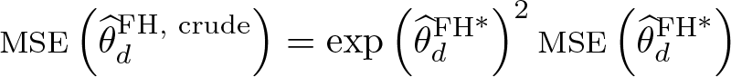
The FH model assumes linearity and normality of its two error terms. If there is a violation of these assumptions, a log-transformation of the direct estimator might be an option (Slud and Maiti 2006). Choosing this option requires an appropriate transformation of the variance of the original direct estimator.³ Neves, Silva, and Correa (2013) suggest the transformation,

\begin{matrix} {\hat{θ}}_{d}^{*} = log ({\hat{θ}}_{d}) \\ var ({\hat{θ}}_{d}^{*}) = {({\hat{θ}}_{d})}^{- 2} var ({\hat{θ}}_{d}) \end{matrix}

with ^∗ indicating the transformed scale.

Equation (1) is estimated using ${\hat{θ}}_{d}^{*}$ as the direct estimate and var( ${\hat{θ}}_{d}^{*}$ ) as the estimate for the sampling error variance. To bring the estimated EBLUP and MSE back from the transformed to the original scale, we advise a bias correction (Slud and Maiti 2006; Sugawasa and Kubokawa 2017). fayherriot includes two back-transformation methods: the “crude” method, shown in Neves, Silva, and Correa (2013) and Rao and Molina (2015), and (as the default) the bias correction proposed by Slud and Maiti (2006). For the point estimates, these methods are defined as

\begin{array}{l} {\hat{θ}}_{d}^{FH, crude} = exp {{\hat{θ}}_{d}^{FH *} + 0. 5MSE ({\hat{θ}}_{d}^{F H *})} \\ {\hat{θ}}_{d}^{FH, Slud-Maiti} = exp {{\hat{θ}}_{d}^{FH *} + 0.5 {\hat{σ}}_{u}^{2} (1 - {\hat{γ}}_{d})} \end{array}

with ∗ indicating the transformed scale.

The Slud–Maiti back-transformation relies on MLE for the estimation of $σ_{u}^{2}$ . Because it requires an estimate of ${\hat{γ}}_{d}$ , it is only applicable for in-sample domains. The crude back-transformation can be used for in- and out-of-sample predictions.

For estimating the precision of the back-transformed EBLUPs, Slud and Maiti (2006, 248) developed an MSE estimator when using the log-transformation. The crude method uses the estimates in the transformed scale and the following back-transformation:

MSE ({\hat{θ}}_{d}^{FH, crude}) = exp {({\hat{θ}}_{d}^{FH *})}^{2} MSE ({\hat{θ}}_{d}^{FH *})

2.5 Overview of functionalities

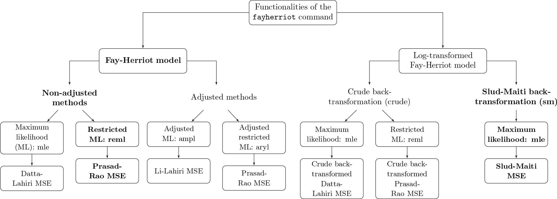
Figure 1 gives an overview of the functionalities of the fayherriot command. Additionally, the arcsine square root transformation can be used for proportions, and fayherriot returns back-transformed EBLUPs and corresponding boundaries of bootstrap confidence intervals. For a detailed description, we refer to Casas-Cordero Valencia, Encina, and Lahiri (2016, 394–397) and Schmid et al. (2017, 1173–1177).

Figure 1.

Functionalities of the fayherriot command. The two lowest levels describe the estimation methods of σu ² and the corresponding MSE estimators, respectively. The default options are written in bold.

3 The fayherriot command

3.1 Syntax

fayherriot runs in Stata 12 and later versions. The syntax is

fayherriot depvar $[v a r l i s t] [i f] [i n]$ , variance( varname ) sigmamethod( method ) logarithm arcsin biascorrection( method ) initialvalue( # ) reps( # ) level( # ) eblup( name ) mse( name ) gamma nolog

The command runs on datasets on the domain level with one observation per domain. depvar is the direct estimate, ${\hat{θ}}_{d}$ (in the documentation, theta), and varlist corresponds to the auxiliary explanatory variables, x _d (in the documentation, X).

3.2 Options for fayherriot

variance( varname ) determines the variable containing the sampling error variances, $σ_{e_{d}}^{2}$ . This variance is assumed to be known in the model. However, it often needs to be estimated from the data. One possibility is to use the estimated variance of the direct estimator specified in depvar for each domain. Whenever the direct estimator needs to be logarithmized with logdepvar = log(depvar), the estimated variance can be modified as logvar = var/(depvar²) (Neves, Silva, and Correa 2013). In case the estimate is transformed by the arcsine transformation theta arcsine = asin $(\sqrt{{\hat{θ}}_{d}})$ , the estimated variance can be approximated by sigma2 e arcsine = 1/(4×effsample) with effsample being the effective sample size (Jiang et al. 2001). The effective sample size is an estimate of the sample size that a survey based on simple random sampling would have to have the same sampling error as the currently used survey with the corresponding sampling design. It can be estimated by the division of the sample size and the design effect (Lohr 2010, 239). variance() is required.

sigmamethod( method ) specifies the method for the estimation of the variance of the random effect $σ_{u}^{2}$ : reml, mle, ampl, or aryl. The default is sigmamethod(reml). If a zero estimate is received for the variance—which is more likely when the number of domains is small—the adjusted maximum-likelihood methods ampl (Li and Lahiri 2010) and aryl (Yoshimori and Lahiri 2014) may help to estimate strictly positive variances.

logarithm indicates that the dependent variable in depvar is the log-transformed direct estimate. A log-transformed FH model is suitable when the linearity or normality assumption of the error terms is not fulfilled. logarithm automatically back transforms EBLUP and MSE to the original scale.

arcsin indicates that the dependent variable in depvar is the direct estimate transformed by the arcsine square root transformation. This transformation is especially suitable when the indicator of interest is a proportion confined to the [0, 1] interval. arcsin automatically back-transforms EBLUP and the boundaries of the bootstrap confidence interval to the original scale.

biascorrection( method )determines the method for the back-transformation of EBLUP and MSE in a log-transformed FH model. The EBLUPs and MSEs in the transformed scale can be back-transformed using the bias correction proposed by Slud and Maiti (2006), which is set as a default, and a crude bias correction (Neves, Silva, and Correa 2013; Rao and Molina 2015). When the arcsine transformation is used, the EBLUP and the boundaries of the confidence interval are, by default, back-transformed by the inverse transformation as proposed in Casas-Cordero Valencia, Encina, and Lahiri (2016), and thus no method needs to be specified.

initialvalue( # ) sets the initial value of the optimization algorithm for estimating the variance of the random effect $σ_{u}^{2}$ to #. The default is initialvalue(0.0).

reps( # )sets the number of bootstrap repetitions for the confidence intervals to #. The default is reps(100). The confidence intervals are returned if arcsin is specified.

level( # ) sets the confidence level of the bootstrap confidence intervals to #. The default is level(95), which corresponds to a 95% confidence level.

eblup( name ) stores the EBLUP estimates in the variable name. For in-sample domains, the EBLUPs are defined as eblup() = $x_{d}^{T} \hat{β} + {\hat{u}}_{d}, where x_{d}^{T} \hat{β}$ are the estimated fixed effects and ${\hat{u}}_{d}$ is the estimated random effect. The EBLUP can also be expressed as the weighted average of the direct estimator and a synthetic part, eblup() $= {\hat{γ}}_{d} \times {\hat{θ}}_{d} + (1 - {\hat{γ}}_{d}) x_{d}^{T} \hat{β}$ . For out-of-sample domains, the EBLUP shrinks to the synthetic part, eblup() $= x_{d}^{T} \hat{β}$ .

mse( name ) stores the MSE estimates in the variable name. The MSE depends on the estimation procedure of sigma2 u. For sigmamethod(reml), the MSE estimator relies on Prasad and Rao (1990, 167); for sigmamethod(mle), the MSE estimator relies on Datta and Lahiri (2000, 619); for sigmamethod(ampl), the MSE estimator relies on Li and Lahiri (2010, 886); and for sigmamethod(aryl), the MSE estimator relies on Yoshimori and Lahiri (2014). For the log-transformed FH model under the Slud– Maiti bias correction, the MSE is defined as in Slud and Maiti (2006, 248). It is only applicable to in-sample domains. Under the crude bias correction, for in- and out-of-sample domains, mse(eblup backtransformed) = exp(EBLUP)²×mse(EBLUP) (Neves, Silva, and Correa 2013). In case arcsin is chosen, upper and lower bounds of bootstrap confidence intervals (Casas-Cordero Valencia, Encina, and Lahiri 2016, 394–397; Schmid et al. 2017, 1173–1177) are returned.

gamma reports summary statistics of the shrinkage factor, ${\hat{γ}}_{d} = {\hat{σ}}_{u}^{2} / ({\hat{σ}}_{u}^{2} + σ_{e_{d}}^{2})$ , where is the estimated variance of the random effect and $σ_{e_{d}}^{2}$ is the sampling error variance of each domain provided in variance( varname ).

nolog suppresses the display of the iteration log of the optimization algorithm.

3.3 predict after fayherriot

Syntax

The syntax for predict following fayherriot is

predict [type] newvar [if] [in] [ , eblup mse reps( # ) level( # ) ehat estandard uhat gamma cvdirect cvfh ]

Options

eblup generates the EBLUPs as defined above; this is the default.

mse generates estimates for the MSE or the boundaries of the confidence interval as defined above.

reps( # ) sets the number of bootstrap repetitions for the confidence intervals to #. The default is reps(100).

level( # ) sets the confidence level of the bootstrap confidence intervals to #. The default is level(95), which corresponds to a 95% confidence level.

ehat calculates the residuals. The residuals are defined as ${\hat{e}}_{d} = (1 - {\hat{γ}}_{d}) \times ({\hat{θ}}_{d} - x_{d}^{T} \hat{β})$ , where ${\hat{θ}}_{d}$ corresponds to depvar.

estandard calculates the standardized residuals defined as ${\hat{e}}_{d} / \sqrt{σ_{e_{d}}^{2}} .$

uhat calculates the random effects. The random effects are defined as ${\hat{u}}_{d} = {\hat{γ}}_{d} \times ({\hat{θ}}_{d} - x_{d}^{T} \hat{β}) .$

gamma generates the shrinkage factor as defined above.

cvdirect calculates the coefficient of variation (CV) of direct estimates. cvdirect = $100 \times \sqrt{σ_{e_{d}}^{2}} / {\hat{θ}}_{d}, where {\hat{θ}}_{d}$ corresponds to depvar and $σ_{e_{d}}^{2}$ is the sampling error variance provided in variance(). In case logarithm is specified, cvdirect $= 100 \times \sqrt{σ_{e_{d}}^{2'}} / θ^{'} with {\hat{θ}}^{'} = exp ({\hat{θ}}_{log}), and σ_{e_{d}}^{2'} = var ({\hat{θ}}_{log}) \times {({\hat{θ}}^{'})}^{2}$ . In case arcsin is chosen, the CV for the direct estimate cannot be returned because the direct variance in the original scale is unknown within the fayherriot command.

cvfh calculates the CV based on EBLUPs: cvfh = 100 × $\sqrt{mse}$ / eblup. In case arcsin is chosen, the CV for the EBLUP cannot be returned because no MSE estimation is provided.

3.4 Stored resultssss

4 Example

We use the FH model to estimate households’ material well being in 2015 in Germany: at the level of federal states (16 divisions), planning regions (96 divisions), and districts (402 divisions). Material well being is defined as region-specific average equivalent income, that is, household disposable income divided by the Organisation for Economic Co-operation and Development modified scale (Hagenaars, de Vos, and Zaidi 1994).

Following the policies used by several statistical agencies to evaluate the precision of the regional estimates, we rely on the CV, which is the standard error of the estimate divided by the estimate (in percent). For instance, Statistics Canada releases data without warning about low precision if the CV is below 16.5% (Statistics Canada 2013; Eurostat 2013).

4.1 Data description and direct estimates

We derive the direct estimates from the German Socio-Economic Panel (SOEP), which is a household survey covering about 15,000 households per year (Goebel et al. 2019).

Table 1 provides the division-specific numbers of SOEP households. Sample sizes by federal states are large (median: 624), ranging from 114 to 3,159 observations. Sample sizes by planning regions are considerably smaller (median: 132), ranging from 32 to 665 observations. Sample sizes by districts range from 10 to 648 observations (median: 32).⁴ Because of small sample sizes, we expect that many direct estimates for planning regions and districts are measured with high imprecision.

Table 1.

Number of regions and sample sizes

		Sample-size distribution
Regional division	Number of regions	Minimum	p10	p25	p50	Maximum
Federal states	16	114	144	444	624	3159
Planning regions	96	32	61	88	132	665
Districts	357	10	14	20	32	648

Note: Data are from SOEP v33.1. Computations are our own.

For each regional level, table 2 provides direct estimates of mean equivalent income and coefficients of variation, our precision indicator.⁵ The table suggests considerable regional heterogeneities in material well being. Across federal states, mean equivalent income ranges from €1,362 to €1,863; across planning regions, from €1,298 to €2,101; and across districts, from €1,023 to €2,976. As expected, coefficients of variation increase as we move to smaller regional levels. In line with the policy of Statistics Canada, not all estimates could be reported for the planning regions and the districts without warning of low precision. In the following, we show how this can be achieved using the FH model. In particular, we can a) improve the precision of all estimates and b) receive estimates for the districts without a direct estimator.

Table 2.

Summary of mean equivalent household income and coefficients of variation by regional level

Regional division			p25	p50	p75	p90	Maximum
(A) Mean equivalized household income
Federal states	1362	1398	1492	1683	1777	1841	1863
Planning regions	1298	1400	1495	1664	1780	1898	2101
Districts	1023	1311	1463	1641	1847	2049	2976
(B) Coefficient of variation
Federal states	0.6	0.8	1.4	2.2	3.8	6.4	8.0
Planning regions	1.5	3.4	4.1	5.3	7.2	9.0	18.2
Districts	2.2	5.8	7.6	10.2	13.6	16.7	42.5

Note: Data are from SOEP v33.1. Computations are our own.

4.2 Estimation using fayherriot

For fitting the FH model, we rely on the direct estimates of average equivalent incomes (table 2); their sampling error variances, $σ_{e_{d}}^{2}$ ; and region-specific explanatory variables. The set of explanatory variables in this example includes the unemployment rate, the share of the population older than 65 years, and per-capita income tax revenue.⁶

FH model for the planning regions

In the following, we detail the application of fayherriot at the level of planning regions. In this example, all regions are sampled and the model assumptions are fulfilled. The underlying dataset includes 96 observations (one observation per region):

To fit the FH model, we type

The syntax of the command is inline with the familiar Stata regression syntax: income contains the direct estimates of mean equivalent income and is regressed on the regional explanatory variables unemployment, incometax, and share65. variance() specifies the variable containing the sampling error variances, directvariance. We specify the gamma option to display summary statistics of shrinkage factors ${\hat{γ}}_{d}$ . nolog suppresses the iteration log of the optimization algorithm.

N in sample indicates that the full set of 96 planning regions was used in the estimation. FH R-squared is an indicator for the goodness of fit of the FH model, proposed by Lahiri and Suntornchost (2015, 317, Adj $R_{h}^{2}$ ). Similarly to the standard R ², it expresses the explained variation of income in relation to the total variation, while taking into account that some variation in income is due to the sampling error. In this example, about 78% of the variation is explained.

The variance of the random effects, ${\hat{σ}}_{u}^{2}$ = 4683.72, is estimated using the REML approach (the default). Together with the sampling error variances $σ_{e_{d}}^{2}$ , it determines the shrinkage factor ${\hat{γ}}_{d}$ . The shrinkage factor shows how direct estimates and model predictions are weighted when calculating the EBLUP. Large values of ${\hat{γ}}_{d}$ mean that a large weight is given to the direct estimate ${\hat{θ}}_{d} .$ In our example, the distribution of ${\hat{γ}}_{d}$ ranges from 0.0465 to 0.8844 with its median being 0.3726. So for some regions, the EBLUP relies strongly on the model predictions (small value of ${\hat{γ}}_{d}$ ) and strongly on the direct estimator for others (large value of ${\hat{γ}}_{d}$ ). The Shapiro–Wilk test for normality shows that neither normality of the realized residuals, ${\hat{e}}_{d}$ , nor of the random effects, ${\hat{u}}_{d}$ , is rejected. Hence, the model assumptions are not violated.

Log-transformed FH model for the districts

In the district-level analysis, not all regions are sampled, and the normality assumption of the model is violated. Hence, we log-transform equivalent incomes and the variances of the sampling error,

and fit the log-transformed FH model:

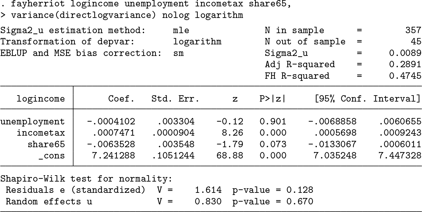
By specifying the logarithm option, fayherriot transforms the estimated EBLUP and MSE back to the original scale. Because we did not specify the bias-correction method, the estimation method is MLE and the bias correction follows Slud and Maiti (2006) (see figure 1). In this default setting, only estimates for the 357 in-sample districts are calculated. biascorrection(crude) could be specified to obtain in- and out-of-sample estimates.

4.3 Comparison of direct and FH estimates

Next we compare the direct with the FH point estimates (EBLUP) and assess their precision. There are two equivalent ways to obtain the EBLUPs and their level of precision (MSE). The first is specifying the eblup( varname ) and mse( varname ) options (here done for the planning regions):

. fayherriot income unemployment incometax share65,

> variance(directvariance) nolog eblup(eblupROR) mse(mseROR)

The second is using the postestimation predict routine directly after the fayherriot command:

. predict eblupROR, eblup

. predict mseROR, mse

An additional feature of predict is that it provides the CV for the direct and FH estimates.

. predict cvROR_FH, cvfh

. predict cvROR_direct, cvdirect

To assess the magnitude of adjustments, figure 2 presents the ratios of EBLUPs and direct estimates against region-specific sample sizes.⁷ For federal states, the ratios are all close to 1, suggesting small adjustments of the direct estimator. For planning regions and districts, adjustments are larger, which is an expected result given smaller sample sizes of these domains.

Figure 2.

Ratio of the EBLUP to the direct (income) estimates plotted against regional sample sizes for all three regional divisions—federal states, planning regions, and districts. Only in-sample domains are plotted. Data are from SOEP v33.1. Computations are our own.

To assess the gain in precision, figure 3 provides box plots of coefficients of variation for the direct and FH estimates. The horizontal line indicates the threshold of 16.5 suggested by Statistics Canada. For the direct estimates, several CVs at the district and planning region levels exceed the threshold. For the FH estimates, in contrast, CVs for all regional levels are under the threshold.

Figure 3.

Box plots of the distribution of the coefficients of variation for the federal states, the planning regions, and the districts. The horizontal line indicates the precision threshold of 16.5%. Only in-sample domains are plotted. Data are from SOEP v33.1. Computations are our own.

5 Conclusion

We implemented the FH model in Stata. It is a small-area estimation technique and aims at improving the precision of direct estimators from a survey by using additional domain-level covariate information. We introduced the fayherriot command and provided an application to regional heterogeneities in material well being in Germany. The results showed that the precision of the FH model estimates is markedly higher than that of the direct estimates.

7 Programs and supplemental materials

Supplemental Material, st0570 - The fayherriot command for estimating small-area indicators

Supplemental Material, st0570 for The fayherriot command for estimating small-area indicators by Christoph Halbmeier, Ann-Kristin Kreutzmann, Timo Schmid and Carsten Schröder in The Stata Journal

Footnotes

6 Acknowledgments

Halbmeier and Schröder thank Johannes König for his valuable remarks and comments, as well as Paul Brockmann, Deborah Anne Bowen, and Fabian Nemeczek for excellent research assistance. Kreutzmann and Schmid gratefully acknowledge support by the German Research Foundation within the project QUESSAMI (281573942) and the MIURDAAD Joint Mobility Program (57265468). We thank the editor and the referee for their constructive comments that helped to improve the article.

7 Programs and supplemental materials

To install a snapshot of the corresponding software files as they existed at the time of publication of this article, type

Notes

References

Battese

G. E.

Harter

R. M.

Fuller

W. A.

1988. An error-components model for prediction of county crop areas using survey and satellite data. Journal of the American Statistical Association 83: 28–36.

Brown

Chambers

Heady

Heasman

2001. Evaluation of small area estimation methods—An application to unemployment estimates from the UK LFS. In Symposium 2001—Achieving data quality in a statistical agency: A methodological perspective. Ottawa: Statistics Canada.

Bundesinstitut für Bau-, Stadt-, und Raumforschung. 2017. Indikatoren und Karten zur Raumund Stadtentwicklung. Datenlizenz Deutschland - Namensnennung - Version 2.0. http://www.inkar.de/.

Casas-Cordero Valencia

Encina

Lahiri

2016. Poverty mapping for the Chilean comunas. In Analysis of Poverty Data by Small Area Estimation, ed. Pratesi

, 379–403. Hoboken, NJ: Wiley.

Corral

Seitz

Azevedo

J. P.

Nguyen

M. C.

2018. fhsae: Stata module to fit an area level Fay–Herriot model. Statistical Software Components, S458495, Boston College Department of Economics. https://ideas.repec.org/c/boc/bocode/s458495.html.

Datta

G. S.

Lahiri

2000. A unified measure of uncertainty of estimated best linear unbiased predictors in small area estimation problems. Statistica Sinica 10: 613–627.

Eurostat. 2013. Handbook on precision requirements and variance estimation for ESS households survey. Methodologies and working papers, European Union.

Fay

R. E.

III Herriot

R. A.

1979. Estimates of income for small places: An application of James–Stein procedures to census data. Journal of the American Statistical Association 74: 269–277.

Goebel

Grabka

M. M.

Liebig

Kroh

Richter

Schröder

Schupp

2019. The German Socio-Economic Panel (SOEP). Journal of Economics and Statistics 239: 345–360.

10.

Hagenaars

A. J. M.

de Vos

Zaidi

M. A.

1994. Poverty Statistics in the Late 1980s: Research Based on Micro-data. Luxembourg: Office for the Official Publications of the European Communities.

11.

Horvitz

D. G.

Thompson

D. J.

1952. A generalization of sampling without replacement from a finite universe. Journal of the American Statistical Association 47: 663–685.

12.

Huang

E. T.

Bell

W. R.

2012. An empirical study on using previous American Community Survey data versus Census 2000 data in SAIPE models for poverty estimates. Research Report Series Statistics #2012-04, U.S. Census Bureau. https://www.census.gov/content/dam/Census/library/working-papers/2012/adrm/rrs2012-04.pdf.

13.

Jiang

Lahiri

Wan

S.-M.

C.-H.

2001. Jackknifing in the Fay–Herriot model with an example. In Proc. Sem. Funding Opportunity in Survey Research, 75–97. Washington, DC: Bureau of Labor Statistics.

14.

Lahiri

Suntornchost

2015. Variable selection for linear mixed models with applications in small area estimation. Indian Journal of Statistics 77: 312–320.

15.

Leadership Council of the Sustainable Development Solutions Network. 2015. Indicators and a monitoring framework for the Sustainable Development Goals. Report to the Secretary General of the UN, United Nations.

16.

Lahiri

2010. An adjusted maximum likelihood method for solving small area estimation problems. Journal of Multivariate Analysis 101: 882–892.

17.

Lohr

S. L.

2010. Sampling: Design and Analysis. 2nd ed. Boston: Cengage Learning.

18.

Molina

Rao

J. N. K.

2010. Small area estimation of poverty indicators. Canadian Journal of Statistics 38: 369–385.

19.

Neves

Silva

Correa

2013. Small domain estimation for the Brazilian service sector survey. Estadística 65: 13–37.

20.

Piacentini

2014. Measuring income inequality and poverty at the regional level in OECD countries. OECD Statistics Working Papers 2014/03, OECD Publishing. https://doi.org/10.1787/5jxzf5khtg9t-en.

21.

Powers

Basel

O’Hara

2008. SAIPE county poverty models using data from the American Community Survey. https://www.census.gov/content/dam/Census/library/workingpapers/2008/demo/powersbaselohara2008asa.pdf.

22.

Prasad

N. G. N.

Rao

J. N. K.

1990. The estimation of the mean squared error of small-area estimators. Journal of the American Statistical Association 85: 163–171.

23.

Rabe-Hesketh

Skrondal

2012. Multilevel and Longitudinal Modeling Using Stata. 3rd ed. College Station, TX: Stata Press.

24.

Rao

J. N. K.

Molina

2015. Small Area Estimation. 2nd ed. Hoboken, NJ: Wiley.

25.

Rendtel

1995. Lebenslagen im Wandel: Panelausfälle und Panelrepräsentativität. Frank furt: Campus.

26.

Schmid

Bruckschen

Salvati

Zbiranski

2017. Constructing sociodemographic indicators for national statistical institutes by using mobile phone data: Estimating literacy rates in Senegal. Journal of the Royal Statistical Society, Series A 180: 1163–1190.

27.

Slud

E. V.

Maiti

2006. Mean-squared error estimation in transformed Fay–Herriot models. Journal of the Royal Statistical Society, Series B 68: 239–257.

28.

Statistics Canada. 2013 2013 National Graduate Survey (Class of 2009–2010). Microdata user guide, Statistics Canada.

29.

Sugawasa

Kubokawa

2017. Transforming response values in small area prediction. Computational Statistics & Data Analysis 114: 47–60.

30.

Tzavidis

Zhang

L.-C.

Luna

Schmid

Rojas-Perilla

2018. From start to finish: A framework for the production of small area official statistics. Journal of the Royal Statistical Society, Series A 181: 927–979.

31.

Yoshimori

Lahiri

2014. A new adjusted maximum likelihood method for the Fay–Herriot small area model. Journal of Multivariate Analysis 124: 281–294.

32.

You

Chapman

2006. Small area estimation using area level models and estimated sampling variances. Survey Methodology 32: 97–103.

Supplementary Material

Please find the following supplemental material available below.

For Open Access articles published under a Creative Commons License, all supplemental material carries the same license as the article it is associated with.

For non-Open Access articles published, all supplemental material carries a non-exclusive license, and permission requests for re-use of supplemental material or any part of supplemental material shall be sent directly to the copyright owner as specified in the copyright notice associated with the article.

0.03 MB

0.00 MB