Sage Journals: Discover world-class research

Abstract

Glass fiber felt is produced by flame blowing process, in which primary glass filament splits into glass fiber through the gas jet into the diffusion duct. In the diffusion duct, the velocity difference at axial direction creates a fiber recirculating zone at some position downstream in the duct while affecting the homogeneity of the product. In order to understand the impact of diffusion duct design to the felt forming, numerical simulations with experiment-based boundary conditions were performed to investigate the movement of fiber suspension flow. In the numerical analysis, the fiber slender-body theory is introduced. A visualization method is developed to characterize the uniformity of glass fiber, through charge coupled device camera imaging demonstrating the intensity of glass fiber in the surface of the product. The proposed methodology enabled new design of the diffusion duct, which eliminated the recirculating zone in the duct, resulting in more uniform products.

Keywords

Glass fiber felt flame blowing process fiber suspension flow diffusion duct design numerical simulation

Introduction

The glass fiber felt is a porous material with good temperature and chemical resistance characteristics. Because of its acoustic and thermal insulation properties, glass fiber felt has been widely used in building constructions, transportation, and aerospace applications [1]. When the fiber diameter gets down to 0.5–2.0 µm, it can be used as a high efficiency filter media. Comparing to electrostatically charged synthetic fibers, glass fiber is more durable. Unlike membrane filter [2 –6], which is a screen filter with a defined pore structure, high-porosity glass fiber felts are depth filters with no defined pores [7]. In the particle disposition, the particles accumulate both within the filter and the surface [8,9], increasing the dust-holding capacity. There are three main manufacturing processes for glass fiber, continuous draw, flame blowing process, and centrifugal spinneret blow [10]. Each process imparts to the fiber a unique set of characteristics such as diameter, length, and surface chemistry and structure.

Traditionally, glass fiber felt is produced through flame blowing process as shown in Figure 1. Frits made from recycled glass are screened out to remove any flaw ones, then melt into glass liquid in an electric melting furnace. The viscous melt fluid is drawn through a nickel alloy leak board by a drawing roller to form the primary glass filaments with diameter around 3 mm. Under the airflow jetted from combustion nozzle, the glass filament splits into secondary fibers, namely glass fibers. The glass fibers are carried into diffusion duct under the high-speed airflow from the nozzle. Meanwhile, the secondary airflow generated by the negative pressure from the jet flow entered the duct. Moving along the diffusion duct, the fiber suspension expand its width, and lands on the convey belt. Finally, polypropylene adhesive is sprayed onto glass fibers on conveyor belt, and cured at 180°C to form glass fiber felts.

Figure 1.

Schematic diagram of flame blowing process.

Barchilon and Curtet have reported that an axisymmetric confined jet produced backflow in the presence of velocity difference in cross section [11,12]. They proposed a single dimensionless parameter Craya–Curtet number (C_t). Many researchers have studied the confined jet [13 –17], revealing that the main parameters affecting the recirculating zone in confined jet are the ratio between primary and secondary flows and the distance of the jet to wall in cross section. As illustrated in Figure 2, when the high-speed airflow enters the duct, a recirculating zone at some position downstream can be generated due to the linear velocity difference in the duct [18]. When the recirculating zone moves along the duct, mechanical collisions among fibers occur, resulting in entanglement of the fibers. The more entanglement generated in the diffusion duct, the more inhomogeneity will occur at the surface of the felt. Surface homogeneity is important for product performance. Using filtration application as an example, when the surface of the product is not uniform, i.e., the density distribution varies across the web, the air flow will be easier to pass through the part with low fiber density [19,20], resulting in poor filtration efficiency.

Figure 2.

Characteristics of the flow for coaxial ducted jets.

In flame blowing process, the design of diffusion duct is critical for the final formation of the glass fiber felt. Change in the size and shape of the inlet of diffusion duct contributes to change of Craya–Curtet number in the duct, indicating that the track of air flow in the diffusion duct has been altered and resulting in different glass fiber felt formation.

In the past, studies have been mainly focused on the formation of the glass fiber felt, especially the quality of primary layer [21]. It has been reported that in flame blowing process, the quality of the primary layer is closely related to three process parameters [22]: (i) drawing velocity of the primary fiber to match the velocity at which the filament is fed into the blowing device; (ii) hot gas flow rate; and (iii) gas jet temperature for melting the primary filament. Recently, Yang designed a venturi tube to guide the glass fibers and studied the glass fiber transmission mechanism in the venturi tube [23]. However, there is no reported study on the trajectory of fiber suspension flow in the diffusion duct and the impact of duct design.

In this study, for the first time we reported the simulation using numerical analyses aiming to understand the movement of glass fiber suspension in diffusion duct and the effect of duct design on final felt formation. The outcome can provide guideline for process design and optimization to achieve glass fiber felt product with high quality and good uniformity.

Theory

The goal of the numerical study was to investigate the track of airflow in the diffusion duct. The relationship between the airflow and diffusion duct structure in accordance to fiber slender-body theory was also analyzed.

Simulation

In this study, a three-dimensional structured mesh code, ANSYS code 16.0, was used to calculate the flow in the computational domain, based on the set of Reynolds-averaged Navier–Stokes equations (RANS) [24]. In the RANS approach, the mass conservation equation (1), the momentum conservation equation (2), and the energy conservation equation (3) can form a closed set of equations together with the equations of the turbulence model (equations (4) and (5)).

The mass conservation equation

\frac{\partial ρ}{\partial t} + \nabla \cdot (ρ U) = 0

(1)

The momentum conservation equation

\frac{\partial (ρ U)}{\partial t} + \nabla \cdot (ρ UU) = - \nabla P + \nabla \cdot (µ \nabla U)

(2)

The energy conservation equation

\frac{\partial ρ e}{\partial t} + \nabla \cdot (ρ U e) + \frac{\partial ρ K}{\partial t} + \nabla \cdot (ρ U K) - \nabla \cdot (α_{eff} \nabla e) = - \nabla \cdot (ρ U)

(3)

The closure of the set of the equations is simplified to determine the turbulent viscosity with the introduction of differential equations of the turbulence model. A two-equation k–e RNG turbulence model by Launder and Spalding was applied as shown in equations (4) and (5) [25]:

Additional equations read

\frac{\partial (ρ k)}{\partial t} + \nabla \cdot (ρ k U) = \nabla \cdot (α_{k} µ_{eff} \nabla k) + P_{k} - ρ ε

(4)

and

\frac{\partial (ρ ε)}{\partial t} + \nabla \cdot (ρ ε U) = \nabla \cdot (α_{ε} µ_{eff} \nabla ε) + C_{1 ε} \frac{ε}{k} P_{k} - C_{2 ε}^{*} ρ \frac{ε^{2}}{k}

(5)

where

α_{k}

and

α_{ε}

are the inverse effective turbulent Prandtl numbers,

µ_{eff}

is the effective viscosity,

P_{k}

represents the generation of turbulent kinetic energy due to the mean velocity gradients, and

C_{1 ε}

and

C_{2 ε}^{*}

are model coefficients.

Fiber suspension flow

In numerical analysis, grid must be used to discretize the governing equations in a spatial domain. In this study, the fiber scale is much smaller than the characteristic scale of the flow field. If the flow field and fiber are calculated directly, the amount of computation load is too large to be completed in reasonable time. In order to reduce the amount of computation, Batehelor slender-body theory was introduced [26 –29]. Before calculating the fiber suspension flow, it is necessary to determine the properties of the fiber suspension flow.

The concentration of fiber is mainly represented by fiber number density n and fiber volume fraction ϕ. n is the number of fibers in unit volume suspension flow. ϕ is the volume of all fiber particles in unit volume suspension flow. Their relationship is based on equations (6)

ϕ = (\frac{π}{4} d^{2} L) n

(6)

According to these two parameters n and ϕ, the fiber suspension flow can be classified as below:

When nL³ is less than 1, it is a dilute suspending flow. It indicates that the number of fibers in the cube (the length of the side of the cube is fiber length) is less than 1. Correspondingly, the fiber volume fraction ϕ is less than (d/L)²

When nL³ is between 1 and L/d, it is a semi-dilute suspending flow. It means that in the cube, the number of fibers is more than 1; and in the plane (the edge length of the plane is fiber length), the number of fibers is less than 1. Correspondingly, the fiber volume fraction ϕ is between (d/L)² and (d/L), (d/L)² < ϕ < (d/L).

When nL³ is larger than L/d, the suspending flow is in the state of semi-concentration or dense phase. It means that in the plane, the number of fibers is greater than 1. Correspondingly, the fiber volume fraction ϕ is larger than (d/L).

Batchelor theory uses the lattice model to construct the constitutive equation σ for the dilute fiber suspension flow, which is defined as equation (7)

σ = 2 µ E + µ_{f} : E

(7)

where µ is the viscosity of the fluid and E is the strain rate applied to the solvent fluid tensor. In the dilute fiber suspension flow, it can be expressed as

µ_{f} = µ_{fiber} [< pppp > - \frac{1}{3} I < p p >]

(8)

where I is the unit tensor and P is the direction vector of fiber particles.

µ_{fiber}

represents the additional viscosity due to the presence of fiber particles. “< >” denotes the statistical average of the amount of calculation on the fiber orientation segment. For a dilute fiber suspension flow,

µ_{fiber}

is defined as equation (4) according to Batchelor

µ_{fiber} = \frac{1}{6} π n L^{3} µ ε f (ε)

(9)

where

f (ε)

is used to represent the effect of a finite length-to-diameter ratio, expressed as

f (ε) = \frac{1 + 0.64 ε}{1 - 1.5 ε} + 1.659 ε^{2}

(10)

where Ɛ is defined as in equation (6)

ε = 1 / \ln (2 r)

(11)

The aspect ratio of the fiber, r, is determined by fiber length L and fiber diameter d per equation (7)

r = L / d

(12)

Through equations (9) to (12), $µ_{fiber}$ can be determined and the viscosity of the air flow can be re-defined, resulting in reduction of the amount of computation load.

Experiment

Boundary condition setup

There are three input parameters need to be determined for the simulation: the temperature at the combustion nozzle, the mass flow rate at the inlet of the diffusion duct, and the air suction flow rate at the suction channel.

Platinum rhodium thermocouple was used to measure the temperature at the combustion nozzle. To prevent the damage of the thermocouple caused by the high flow rate, an alloy protective device was developed and used to cover the thermocouple (shown in Figure 3). In our experiment, the temperature at the combustion nozzle was measured to be 1350°C.

Figure 3.

Platinum rhodium thermocouple without (a) and with (b) the designed protection device.

The gas flow out of the combustion nozzle is actually comprised of air flow and burning gas flow. To achieve the optimized combustion at the site, the molar ratio of burning gas and air was set as 1: 3.69.

The flow rate at the nozzle has a direct impact on the fiber diameter in the final product. In order to achieve the fiber diameter range of 0.5–2.0 µm, multiple experiments have been conducted. The flow rate of burning gas was set at 56 m³/h and the gauge pressure was set at 0.03 MPa (i.e., 0.3 atmosphere pressure). Based on the density of burning gas and air, the mass flow rate at the nozzle is calculated as 0.101 kg/s.

The negative pressure in the suction channel draws the glass fiber to conveyor belt. The suction pressure was measured by using a pressure pilot tube in suction channel, and the negative pressure is calculated to be 200 Pa.

Viscosity of fiber suspension flow

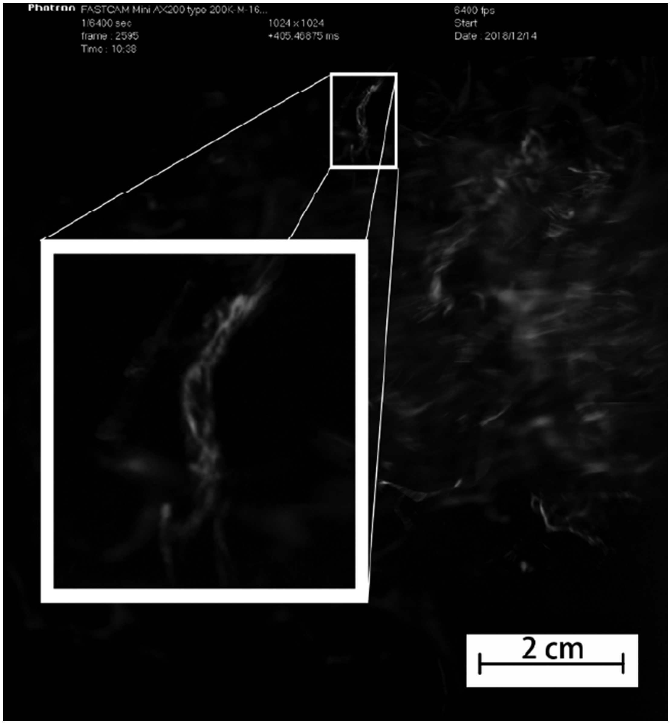
In order to calculate the $µ_{fiber}$ , the fiber properties need to be obtained first. Figure 4 shows the image captured under a high-speed camera, Photron FASTCAM Mini AX200, with resolution of 1024 × 1024 at 6400 frames/s. It should be noted that the fibers described in our study are in fiber bundle format instead of individual fiber.

Figure 4.

Image of the glass fiber captured using high-speed camera.

The diameter and length of fiber were analyzed by Image-pro-plus software. The results indicate that the fiber length L is 1 ± 0.1 cm and fiber diameter d is 400 ± 20 µm. The fiber density number n is the number of fiber in the diffusion duct. It was calculated by the output of glass fiber and the volume of the diffusion duct, with the assumption of all fibers evenly distributed in the diffusion duct. The fiber density number n is, thus, calculated as 8.5 × 10⁵. With the above results, $µ_{fiber}$ can be calculated using equations (9) to (12).

Characterization of glass fiber felt homogeneity

In our experiment and simulation, three designs of diffusion duct were used. As for sample measurement, samples were cut along the cross section of web and averaged results were taken.

Thickness of glass fiber felt

YG141 fabric thickness meter was used for measurement of the glass felt thickness. According to the ISO 9073-2, 10 samples were cut with the size of 130 × 80 mm. A load of 0.02 kPa was applied on the sample and held for 10 s before the measurement of thickness. For each of samples in different duct designs, three production repetitions were measured

CV = \frac{σ}{\bar{X}} \times 100 %

(13)

where σ is expressed as

σ = \sqrt{\frac{\sum_{i = 1}^{n} {(X_{i} - \bar{X})}^{2}}{n - 1}}

(14)

where σ is mean square error of the sample,

\bar{X}

is arithmetic mean of the sample, n is the number of the samples,

and X_{i}

is density of each sample. For each design of diffusion duct, three groups of measurement were taken with 10 samples in each group. The coefficient of variation of each group for product was calculated based on equation (13).

Visualization method for measurement of product homogeneity

Blagojevic [30] developed a visualization method for quantitative measurement of surface uniformity of mineral wool primary layer. The method is based on the acquisition of subsequent images of mineral wool primary layer immediately after the exit from a wool chamber. In this paper, the same methodology was taken using the optical intensity of image as the indicator for sample uniformity. The images were acquired using a black and white charge coupled device (CCD) camera with a resolution of 1024 × 1024 at a frame rate 25/s. The images were digitized using a Photron FASTCAM Viewer frame grabber and analyzed using Image-pro-plus software. The setup of CCD camera and illumination is shown in Figure 5, with imaging size of 120 × 120 mm of sample and constant light source.

Figure 5.

Schematic diagram of charge coupled device camera.

In image analysis of the samples, an average of intensity A in each image was calculated

A = \sum_{l} \sum_{m} E (l, m)

(15)

Here, the intensity of pixels, $E (l, m)$ ranges from 0 to 255, corresponding to the 8-bit resolution of the camera; $l$ and $m$ are the coordinates of the pixels inside the picture.

Results and discussion

Numerical analysis

The goal of the simulation was to test the hypothesis that the track of the fiber suspension flow in the pipe affects the uniformity of the product’s surface. The computational domain included the combustion nozzles, the diffusion duct, the suction channel, and the environment around the production line (shown in Figure 6). The structured mesh with about 5,42,074 nodes was used.

Figure 6.

Illustration of computational domain.

Conditions applied for the simulation are shown as the following:

mass flow inlet: Imposed mass flow rate at inlet nozzles is 0.101 kg/s. Imposed temperature at inlet nozzles is 1350°C.

Pressure outlet: Imposed pressure at the suction channel is −200 Pa. Imposed temperature at the suction channel is 27°C.

Among other parameters used in the simulation, air density, ρ, is temperature dependent. Dynamical viscosity, μ, was calculated through the equations in “Viscosity of fiber suspension flow” section as 7.19 × 10⁻⁵Pa s.

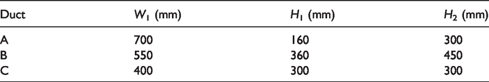
To study the effect of diffusion duct on both simulation and experiment, three designs of diffusion duct were built. The design of diffusion duct is shown in Figure 7 and the specific dimensions are shown in Table 1.

Figure 7.

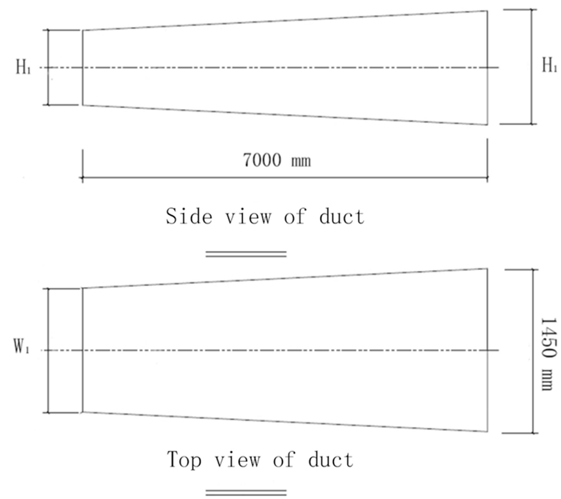
Diagram of diffusion duct (mm).

Table 1.

Design dimensions of diffusion duct.

Duct	W₁ (mm)	H₁ (mm)	H₂ (mm)
A	700	160	300
B	550	360	450
C	400	300	300

In order to compare the simulated results with the experimental results, two easy-to-be measured parameters, temperature and velocity, are selected for comparison. The velocity was measured by using a pilot tube and the temperature was measured by using Platinum rhodium thermocouple at the outlet of the diffusion duct. Table 2 shows the comparison of the airflow velocity and temperature at the outlet of the diffusion duct in simulation and experiment.

Table 2.

Comparison of velocity and temperature between simulation and experiment.

Diffusion duct	Comparison	Average velocity of air flow, m/s	Average temperature of air flow, °C
A	Experiment	6.8	124
A	Simulation	7.5	121
B	Experiment	6.3	98
B	Simulation	7.2	95
C	Experiment	7.4	108
C	Simulation	8.7	106

The data in Table 2 show that the simulated result is in good accordance with the experimental result. It indicates that the boundary condition we used and the setup we applied are appropriate and provide a good numerical analysis of airflow.

Analyzed by CFD-post software, our simulation data enabled the diagrammatical illustration of the airflow pathway, i.e., the flow track. Figure 8 shows the flow track diagram through our simulation for different designs of diffusion duct. For design A and B of diffusion duct, because of the high-speed airflow entering in the duct, the velocity difference at axial direction creates recirculating zones at around 3 m spot from the inlet of the duct. For the design C of diffusion duct, the size of the duct inlet is adjusted through increasing the height and reducing the width. The diagram shows that this size change successfully eliminated the recirculating zone in the duct.

Figure 8.

Flow track diagrams of different diffusion ducts.

Homogeneity analysis

Under production conditions with the same flame temperature and airflow speed, glass fiber felts were produced using three different designs of diffusion duct, A, B, and C. Our first attempt was to use thickness variation as the measurement of sample homogeneity. The coefficients of variation (CV) of the thickness for glass fiber felts produced using three different designs of diffusion duct are shown in Figure 9. Although the homogeneities of fiber distribution in samples A, B, and C are visually different, the difference in CVs for three sets of samples is marginal considering the sample variation (as shown the error bar in Figure 9), indicating that thickness variation is not a good measurement for homogeneity.

Figure 9.

Coefficient of variation of the thickness for glass fiber felts produced using three different designs of diffusion duct. The error bar was calculated based on three production repetitions.

A computer-aided visualization method is adopted for characterization of the homogeneity. The results of image analyses of the samples were shown in Figures 10 to 12 for three diffusion duct designs of A, B, and C. The 2D images of the correspondent samples are shown in Figure 10. The 3D distribution plots of fiber density are shown in Figure 11, which were converted from the 2D images for better demonstration of the density distribution of the sample. The histograms of pixel number versus intensity are shown in Figure 12, which is another way to reflect the intensity variation.

Figure 10.

The 2D images from charge coupled device camera for samples.

Figure 11.

The 3D distribution plots for samples.

Figure 12.

The histograms of intensity for samples.

In the 2D image analysis, the light transmittance reflects the glass fiber density. The lower image intensity has, the higher glass fiber density is. The 3D plots in Figure 12 shows better visualization of the distribution of fiber density in the samples. The wave crests in the 3D plots are the low-density distribution areas, where could be the defect of the product since for filtration application, particles are much easier to pass through the lower density area.

As illustrated in “Visualization method for measurement of product homogeneity” section, the web surface uniformity can be measured through the optical intensity of the sample using CCD camera imaging analysis. The standard deviation of the intensity of products will reflect the level of uniformity, with lower standard deviation indicating more uniformity for the sample. Figure 13 shows the comparison of the standard deviations of intensity for three designs of the diffusion duct. The sample produced through design A diffusion duct has the highest standard deviation, while the sample produced by design C diffusion duct has the lowest standard deviation. It is concluded that image intensity could be used as a good measurement for homogeneity.

Figure 13.

The standard deviations of intensity for glass fiber felts produced using three different designs of diffusion duct. The error bar was calculated based on three production repetitions.

Correlating to our airflow simulation analysis, design A of the diffusion duct has the largest recirculating zone in the airflow track, while design C of the diffusion duct eliminated the recirculating zone. It is our conclusion that reducing the fiber recirculating zone through the design of diffusion duct can effectively reduce the entanglement between the fibers, resulting in more uniform glass fiber felt products.

Conclusions

The paper presents a research of the movement of fiber suspension flow in the diffusion duct and its impact to final product. The flow track of fiber suspension was assessed by numerical analysis. The computer-aided visualization method enabled the evaluation of product homogeneity. A good correlation between the flow track of fiber suspension and the product surface uniformity was determined, indicating the significance of diffusion duct design for the quality of the final product. With the experiments of three different designs of diffusion duct, our study demonstrated that the uniformity of glass fiber felt product can be improved by reducing the recirculating zone in the duct.

In the simulation analysis, we noticed that the density of the fiber suspension has impact to the movement of the fiber suspension flow in diffusion duct. Although the Batchelor slender-body theory was adopted, there is still discrepancy between the simulation and the experimental measurement. In the future work, a better fiber suspension flow theory should be developed and be applied to simulation for flame blow process.

Footnotes

Declaration of conflicting interests

The author(s) declared no potential conflicts of interest with respect to the research, authorship, and/or publication of this article.

Funding

The author(s) received no financial support for the research, authorship, and/or publication of this article.

ORCID iDs

Chi Zou

Yongsheng Liu

Appendix

References

Yang

, et al. Acoustic properties of glass fiber assembly-filled honeycomb sandwich panels. Compos Part B Eng 2016; 96: 281–286.

Guo

, et al. Ultra-thin double Janus nanofiltration membrane for separation of Li+ and Mg2+: “drag” effect from carboxyl-containing negative interlayer. Sep Purif Technol 2020; 230: 115567.

Liu

, et al. Applications, effects and the prospects for electrospun nanofibrous mats in membrane separation. J Mater Sci 2020; 55: 1–32.

, et al. Photocatalytic antifouling PVDF ultrafiltration membranes based on synergy of graphene oxide and TiO2 for water treatment. J Membr Sci 2016; 520: 281–293.

Zhang

, et al. Improved hydrophilicity, permeability, antifouling and mechanical performance of PVDF composite ultrafiltration membranes tailored by oxidized low-dimensional carbon nanomaterials. J Mater Chem A 2013; 1: 3101–3111.

Zhang

, et al. Synergetic effects of oxidized carbon nanotubes and graphene oxide on fouling control and anti-fouling mechanism of polyvinylidene fluoride ultrafiltration membranes. J Membr Sci 2013; 448: 81–92.

Imbabi

MS.

Modular breathing panels for energy efficient, healthy building construction. Renew Energy 2006; 31: 729–738.

Sakano

, et al. Particle collection of medium performance air filters consisting of binary fibers under dust loaded conditions. Sep Purif Technol 2000; 19: 145–152.

John

Reischl

Measurements of the filtration efficiencies of selected filter types. Atmos Environ 1978; 12: 2015–2019.

10.

Bauer

Manville

Properties of glass fiber for filtration: Influence of forming process. Int Nonwovens J 2004; os-13: 1558925004os-13.

11.

Barchilon

Curtet

Some details of the structure of an axisymmetric confined jet with backflow. J Basic Eng 1964; 86: 777.

12.

Craya

Curtet

On the spreading of a confined jet. CR Acad Sci Paris 1955; 241: 621–622.

13.

Nathan

GJ.

Statistical properties of turbulent free jets issuing from nine differently-shaped nozzles. Flow Turbul Combust 2010; 84: 583–606.

14.

Kalt

Nathan

GJ.

On turbulent jets issuing from notched-rectangular and circular orifice plates. Flow Turbul Combust 2010; 84: 565–582.

15.

Rahman

Tay

GFK

Tachie

MF.

Effects of nozzle geometry on turbulent characteristics and structure of surface attaching jets. Flow Turbul Combust 2019; 103: 797–825.

16.

Singh

Sundararajan

Bhaskaran

KA.

Mixing and entrainment characteristics of circular and noncircular confined jets. J Fluids Eng 2003; 125: 835–842.

17.

Xiao

, et al. Numerical investigation on the recirculation in annular jet pumps. J Mech Sci Technol 2013; 27: 1603–1609.

18.

Launder

Spalding

DB.

The numerical computation of turbulent flow computer methods. Comp Methods Appl Mech Eng 1974; 3: 269–289.

19.

Kang

, et al. Modeling of fibrous filter media for ultrafine particle filtration. Sep Purif Technol 2019; 209: 461–469.

20.

Chang

, et al. Development of composite filters with high efficiency, low pressure drop, and high holding capacity PM2.5 filtration. Sep Purif Technol 2019; 212: 699–708.

21.

Sirok

Blagojevic

Novak

Influence of blow away velocity field on the primary layer fibre structure in the mineral wool production process. Glass Technol 2002; 43: 188–194.

22.

Novitskii

Efremov

MV.

A study of the fiber blowing process in the production of mineral wool. Refract Ind Ceram 2006; 47: 121–124.

23.

Yang

, et al. Comparing the uniformity of light glass fiber felt based on process improvement, microstructural forming mechanism and physical properties. Text Res J 2019; 89: 3447–3456.

24.

Patankar

Numerical heat transfer and fluid flow. Series Comput Methods Mech Thermal Sci 1980; 67: 11–17.

25.

Launder

Spalding

DB.

The numerical computation of turbulent flows. Comput Methods Appl Mech Eng 1974; 103: 456–460.

26.

Johnson

RE.

An improved slender-body theory for stokes flow. J Fluid Mech 1980; 99: 411–431.

27.