Sage Journals: Discover world-class research

Abstract

In this article, a numerical method to predict textile geometry is derived using a technique based on finite elements (FEs). A geometric modeling package is used to represent an initial geometry of the yarns within the textile. The yarn mid-surface is then represented using plate elements, with the yarn thickness and cross-section being reconstructed from this mid-surface. The bending and tensile aspects of the yarn behavior are represented by separate features of the plate elements and the total energy for the system is minimized. Contacts are modeled using a penalty method, where the contact force is proportional to penetration distance. Once geometry correction has been achieved by solving the FE problem, the geometric model of the textile is corrected to take into account the predicted movements of the yarns. For validation purposes, the method is applied to two-dimensional (2D) and three-dimensional (3D) weaves and compared against images of the real fabrics. Agreement between predictions and images is good for the 3D weave and excellent for the 2D weave.

Keywords

textiles composites 3D weaving

Introduction

In order to perform numerical simulations to predict properties of a textile structure, a description of its geometry is required. The importance of the geometrical accuracy depends largely on the type of simulation (e.g., mechanical, flow, heat transfer, etc.). This article aims to provide a fast method to predict the geometry of a wide variety of textile types as accurately as possible, so that its importance for any given simulation can be determined in future studies.

The principles of finite element (FE) analysis, which underlies the present approach, have been described in numerous texts, notably the definitive works by Zienkiewicz et al. [1,2] and by Bathe [3], and are summarized in a range of shorter texts such those by Becker [4] and Gallagher [5]. There have been several studies on the use of three-dimensional (3D) continuum FEs to model yarns to predict mechanical properties of textiles [6–11]. Some of the issues with using 3D continuum elements are:

Simulations take a long time to perform primarily due to the complexity of the contact algorithm.

Simulations require a substantial amount of manual effort to define due to a lack of robustness in the contact algorithm.

Bending behavior of yarns cannot be represented accurately with 3D continuum elements [9] due to their highly discontinuous structure.

There have also been numerous studies on the use of analytical techniques to predict fabric geometry and mechanical behavior based on textile mechanics [12–16]. While these techniques are generally robust and fast, they tend to be specific to particular textile architectures and are not easily extended to new textile types. Hivet and Boisse [17] describe a geometric modeling approach which is applied to a variety of two-dimensional (2D) textiles. Although this study relates to the modeling and mechanics of dry textiles, it should be noted that a great deal of work also exists on the mechanics of textile composites (see, for example, the textbook by Bogdanovich and Pastore [18], and the review by Crookston et al. [19]).

The method presented in this article takes ideas from both the analytical and FE textile modeling techniques introduced above, and consists of several stages carried out in sequence:

An initial geometry is defined as one which should contain an accurate description of the yarn interlacement, yarn widths, yarn heights, and a first approximation for the cross-sectional shape, but it need only contain approximate yarn path and yarn twist as these will be predicted by the algorithm.

Based upon this geometry, a FE model of the yarns is constructed, representing the yarns via shell FEs placed at their mid-surfaces.

The total strain energy from bending, twisting, and tensile deformation is minimized within a simplified FE analysis in order to obtain the true yarn paths.

The original yarn geometry is modified to take into account the changes to the yarn paths and cross-sections predicted by the FE model.

This method will be applied to 2D and 3D weaves, and validated against cross-sectional images of these fabrics to assess the accuracy of the method.

Initial geometric modeling and meshing

The topology and approximate geometry of the textile are modeled using the authors' open-source geometrical modeling software package TexGen [9,20]. In its current form, this consists of a library of functions for establishing and manipulating almost any kind of repeating textile geometry; it may be controlled either via a graphical user interface or using an application programming interface. In the present approach, the mid-surfaces of the yarns in the model are extracted by defining the z-direction as perpendicular to the plane of the textile (Figure 1) and finding the surface containing points mid-way between intersections of the upper and lower surfaces of the yarn with arbitrary lines in the z-direction (Figure 2).

Figure 1.

Textile unit cell coordinate system.

Figure 2.

Mid-surface of a single yarn.

The meshing of these surfaces must be done in such a way that pairs of matching nodes (i.e., nodes with matching x–y-coordinates) occur on the mid-surfaces of each pair of yarns which cross (Figure 3), in order to simplify the contact algorithm necessary for the solving stage.

Figure 3.

Matching mid-surface meshes of two crossing yarns.

The method used to create such a mesh will be described using a plain weave for illustration purposes (Figure 4). Note that the method is applicable to fabrics, where crimp is not so extreme that any yarn becomes perpendicular (or nearly perpendicular) to the plane of the fabric. An example which challenges but does not violate this rule is presented in ‘3D orthogonal woven textile’ section.

Figure 4.

Illustration of the steps taken to create the mid-surface mesh for a plain woven fabric: (a) Textile fabric unit cell, (b) Edges identified (c) Edges projected to the XY-plane, (d) Basic regions identified, (e) Regions meshed in 2D and (f) Mesh projected back to yarn mid-surfaces.

Identifying edges

The objective of this stage is to identify the yarn perimeter when viewed along the z-axis. This is done numerically by identifying a series of edge segments from the triangulated surface within the TexGen model having opposing z-components of their normal directions [9]. Each edge segment in the surface mesh is shared by two triangular facets. If the z-components of the two triangular facets' normals have opposite sign, then they are identified as belonging to the perimeter.

The result of the algorithm applied to the fabric shown in Figure 4(a) is shown in Figure 4(b).

Projecting edges

The edges are projected onto the x–y-plane by setting the z-component of all nodes equal to zero, and the resulting skeletal mesh is simplified by removing duplicate segments, unconnected nodes, etc. At the end of this process, each node should be shared by at least two segments.

Identifying basic regions

From the projected edges, a series of basic regions can be identified along with the encompassing region (Figure 5). A basic region is defined as a region bounded by segments forming a polygon which does not contain any other segments or nodes. The region encompassing the basic region can be distinguished from its constituent basic regions by the different directions of the encompassing edge vectors and hence the opposite sign of the area enclosed; this condition arises because of the nature of the search algorithm used to determine the perimeter.

Figure 5.

Identifying basic regions: (a) Basic region and (b) Encompassing region.

Figure 4(d) shows the basic regions identified from the segments in Figure 4(c).

Meshing basic regions

The triangulation of a 2D polygon is a well-established process known as Delaunay refinement [21] and is accomplished here using the third-party library, Triangle [22]. Figure 4(e) shows the basic regions meshed using Triangle given the input shown in Figure 4(d). The resolution of the mesh can be specified at this stage, affecting the accuracy of the solution and the required solution time.

Creating mid-surfaces

The mid-surfaces of each yarn are created by projecting the nodes of each triangular element in the 2D mesh along the z-axis back onto the original 3D surface mesh (Figure 4(a)). If all three projected nodes intersect with the yarn, a mid-surface element is created, where the nodal coordinates are taken as the average of the intersections with the bottom and top surfaces of the yarn. The final mid-surface mesh is shown in Figure 4(f).

FE formulations

The mid-surfaces of the yarns are meshed with FEs to give them structural properties, making it possible to simulate the bending, tensile, and contact forces, typically present in a textile fabric. Using standard techniques, two special elements are formulated to represent the bending and tensile stiffnesses, respectively, while a simple contact algorithm is used to prevent yarn penetration. The bending and tensile elements could have been combined to form a single element, but they were kept separate for convenience. The bending and tensile behaviors of a multifilament tow are uncoupled due to the symmetry of each filament and due to the initially planar nature of each element. This is assumed because the filaments are essentially unconnected and the bending stiffness of the tow is the sum of the filament bending stiffnesses rather than being related to the second moment of area of the tow as a whole. It is important to note that, for simplicity of formulation and computational efficiency, the elements are defined in the plane z = 0, and the tendency for the crimped tows in their out-of-loom state to try to spring back to being straight is modeled via a set of ‘restoring forces’, which are partially opposed by the contact forces which maintain the crimp.

Plate bending element

The plate bending component of the FE model is a simple one drawn from the literature; the concepts, along with the limitations and recommended improvements for this kind of element, are presented in section 12.3 of Ref. [5] and in Ref. [23], though the full definition of the formulation does not appear to have been presented in the current form. A four-noded triangular element with 10 degrees of freedom is formulated, as illustrated in Figure 6. The element has a node at each corner of the triangle each with three degrees of freedom (v, θ_x, and θ_y) and a fourth node possessing a single displacement degree of freedom (v) is located at the centroid of the element.

Figure 6.

Bending element.

For simplicity, the model only considers out-of-plane (z) displacements due to twisting and transverse deformations of the tows; it does not consider movements in the x–y-plane nor inter tow friction or slippage. Each degree of freedom v represents the displacement of the node in the z-direction and θ_x and θ_y represent the change in slope which are defined as

(1)

(2)

The displacement v is assumed to vary over the element by the following shape function, which consists of a complete 2D polynomial of the third degree (Ref. [5], p. 215):

(3)

Consequently, θ_x and θ_y can be expressed in terms of [C_b] using Equations (1) and (2):

(4)

The fourth node with the single displacement degree of freedom is used to increase the number of degrees of freedom to 10, equaling the number of terms in a complete polynomial of third degree.

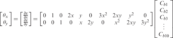
The x- and y-coordinates of the nodes termed (x₁, y₁), (x₂, y₂), (x₃, y₃), and (x₄, y₄) for nodes 1–4, respectively, are known. Following standard procedures and making use of Equations (3) and (4) for calculating displacement and slope at each node, the degrees of freedom (v₁, θ_{x
₁}, θ_{y
₁}, v₂, θ_{x
₂}, θ_{y
₂}, v₃, θ_{x
₃}, θ_{y
₃}, v₄) can be expressed in terms of known nodal coordinates and unknown coefficients [C_b] to give an equation of the form

(5)

where [u_e] is the set of nodal degrees of freedom and [A_b] a matrix containing rows from the matrices in Equations (3) and (4) evaluated at the nodal coordinates, relating the nodal values of the displacements and rotations to the polynomial coefficients.

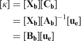
The bending and twisting strains [κ] ([5], p. 329) can also be expressed in terms of [C_b] as follows, by differentiating Equation (3) twice:

(6)

which can be written as

(7)

where [B_b] is a dimension matrix. The bending and twisting moments [M] arising from these strains [κ] can be expressed (for the case where fibers lie in the x- or y-directions, so there are no bending-twisting coupling terms) as follows (from equations 2.66, 4.15 and 4.32 in [24]),

(8)

where D_bx and D_by are the unconstrained bending moduli, (which combine the effects of the material moduli and the tow cross-section dimensions, into a single term but do not depend upon textile architecture other than via the orientation dependence to be introduced via Equation (9)) along the x- and y-axes, respectively. D_bxy is similarly the twisting modulus, and ν_xy and ν_yx the Poisson's ratios^†. In practice, it is more convenient to specify these parameters in terms of a local coordinate system, where the axes 1 and 2 are parallel and perpendicular to the fiber direction, respectively; then, transform the material stiffness matrix from local coordinates to global ones (making use of equation 2.83 in Ref. [24]):

(9)

where D_b1 and D_b1 are the bending moduli, D_b12 the twisting modulus, and ν₁₂ and ν₂₁ the Poisson's ratios, all of which are expressed in the fiber coordinate system, and the transformation matrix [T_b] is expressed in terms of vector

\vec{A}

, which is a unit vector obtained by projecting the fiber orientation vector onto the x–y-plane.

(10)

where terms

{\vec{A}}_{x}

and

{\vec{A}}_{y}

may be regarded as direction cosines of the projected fiber directions in the global axis system. The element stiffness matrix [K_b] is now assembled as follows:

(11)

This integration is approximated numerically using Gaussian quadrature in the usual manner [4].

Plate tensile element

These elements are used to model the apparent transverse ‘stiffness’ (generally termed the geometric stiffness; see, for example, p. 383 of Ref. [5]) of a tensioned yarn rather than to model extensional behavior. For this application, a three-noded triangular tensile element is formulated, where each node has one degree of freedom v. For reasons of computational efficiency and numerical stability, linear variation of displacement is assumed, so that tensile stress and strain are constant over each element. This simplification allows the plate bending and tension-dependent stiffness components of the formulation to be separated, as the values of slopes θ_x and θ_y used here are calculated when needed from the transverse displacements of the vertex nodes, rather than using the rotational degrees of freedom which exist in the bending model only to enforce continuity of slope. The displacement v is assumed to vary over the element in terms of the following shape function containing linear terms in x and y ([5], p. 215):

(12)

The degrees of freedom v₁, v₂, and v₃ can be expressed in terms of known nodal coordinates and unknowns [C_t] following standard procedures, e.g., p. 40 of Ref. [4] as:

(13)

or in a more concise form:

(14)

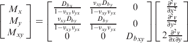
The slope of the element [θ] can also be expressed in terms of [C_t] by differentiating Equation (12) as follows:

(15)

which can be written as

(16)

where [B_t] is a dimension matrix similar to that of the bending element. Tensile forces in a yarn always act along the direction of the fibers, thus, the z-component of a tensile force per unit width σ_z can be expressed in terms of the slope θ and the magnitude of the tensile force per unit width σ₁ (Figure 7):

(17)

Figure 7.

Yarn tension resolved along the z-axis.

Re-arranging and assuming small slope (i.e., sin θ ≈ θ)

(18)

The assumption of small slope is made to keep the equations linear, hence reducing computation time and increasing stability.

In matrix form, this becomes

(19)

where [D_t] fulfills a similar role to the material matrix [D_b] presented for the bending element. It can be constructed in local coordinate space and transformed into global one as follows:

(20)

where [T_t] is the transformation matrix^§ expressed in terms of fiber orientation vector → and σ₁ the known yarn tensile force per unit width.

(21)

The element geometric stiffness matrix [K_t] is then assembled as follows, in a similar manner to that presented in page 2.130 of Ref. [25]:

(22)

Again, this integration is approximated numerically using Gaussian quadrature.

Contact algorithm

Contacts are modeled as modified spring or truss elements with given modulus E connecting two nodes together (Figure 8). The initial rest length L₀ of the spring is equal to

(23)

where t₁ and t₂ represent the thickness at the two nodes (i.e., thickness of the yarn along the z-axis). The length L of the spring at any given time can be expressed in terms of the node's initial z-component of position and displacement v as

(24)

Figure 8.

Diagram of contact elements.

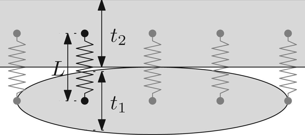
Note that L₀ represents the length when the yarns are just touching and is not necessarily equal to the length L when v₁ and v₂ are zero. The force F opposing the inter yarn penetration exerted by the spring is expressed as

(25)

where A is the area of the spring and is calculated as a third of the sum of the area of the elements sharing the node. The term L₀ in Equation (25) can be problematic as when it equals 0; the force F then becomes infinite. As it is neither necessary nor beneficial for the contact force F to be inversely proportional to the initial rest length L₀, this term is combined with the modulus E to give Ē which is a measure of spring stiffness per unit area. Equation (25) then becomes:

(26)

The modulus Ē (not a traditional Young's modulus, and with units of force/length³) can take one of the two values in order to represent the discontinuous nature of contact stiffness at the onset of contact, depending on whether the spring is in compression (L < L₀, representing penetration) or tension (L > L₀, representing separation). The compressive modulus Ē_c is chosen to be large enough to prevent large penetrations. The tensile modulus Ē_t is made sufficiently small that its presence does not significantly affect the calculated displacements.

In order to use these equations within an FE formulation, a contact stiffness matrix [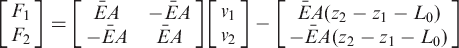K_c] must be formulated. From Equations (24) and (26), the forces F₁ and F₂ exerted on nodes 1 and 2, respectively, can be expressed in matrix form as

(27)

which can be written:

(28)

Boundary conditions

Periodic boundary conditions are applied to the model in order to simulate a unit cell within a much larger fabric. There are two pre-conditions for this to be applicable:

The mid-surface mesh must represent a repeatable unit cell

The mid-surface mesh must be created such that there is a one-to-one mapping between nodes on opposite sides of the unit cell

The degrees of freedom (v, θ_x, and θ_y) of each node lying on the boundary of a unit cell are linked to the degrees of freedom of a corresponding node on the opposite side of the unit cell, so that their values are constrained to be equal.

Solution method

Solution of the problem involves solving a large set of n simultaneous equations which can be represented in matrix form as

(29)

where [x] represents the unknown nodal displacements and [b] the external and/or initial internal forces and moments associated with these degrees of freedom. [K] is the sparsely populated n-by-n global stiffness matrix, which is assembled from the stiffness matrices of the bending and tensile elements in the usual manner [4].

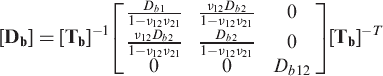
The matrix [b] contains forcing terms that attempt to move the yarns to their unstressed, straight positions on the mid-plane of the textile, opposed by the contact forces which maintain the crimp in the yarns; these forcing terms are calculated as

(30)

where [x₀] is an n-by-1 matrix in which all terms corresponding to the displacement v of a node are set equal to the initial nodal z-coordinate, while the rest of the terms are set to zero.

The contact elements derived in ‘Contact algorithm’ section are then included by adding the terms in the [K_c] and [b_e] matrices to the global [K] and [b] ones, respectively, for each pair of nodes at yarn cross-overs, as illustrated in Figure 3.

In order to insure that there is a unique solution to the problem and prevent rigid body motion, the displacement degree of freedom x_i of a node chosen arbitrarily (specifically, the node associated with the first degree of freedom in the system) is constrained to zero, following the usual procedure of modifying row i of the matrices [K] and [b] to include a single value of 1 and the prescribed (zero) value of x_i, respectively [4].

An extension of this procedure is followed to constrain the degree of freedom x_i to be equal to x_j in applying periodic boundary conditions. Either row i or row j of the matrix [K] is modified; choosing that the row i is modified, entry (i, i) is set to 1, entry (i, j) to −1, and the other entries to zero, and row i of [b] is modified to contain the value 0. This forces the solution to make the values of displacements x_i and x_j to be equal.

Due to the fact that the moduli of the contact elements depend on the relative displacements of the nodes, it is necessary to solve the global system of equations iteratively. The procedure is as follows:

Calculate the stiffness ĒA (used within Equation (26)) of the contact elements (used within Equation (26)) using Ē_c or Ē_t depending upon the contact conditions and hence upon the current nodal positions.

Construct matrices [K] and [b] and solve for [x] using the LU decomposition algorithm implemented in an efficient sparse matrix-solving library, CSparse [26].

Repeat steps 1 and 2 until the modulus of the contact elements has not changed between two successive iterations.

Although there is no theoretical guarantee that this procedure will converge, in practice, it has been found to terminate after a small number of iterations for reasonable values of Ē_c and Ē_t.

Adjusting geometry

Once the deformation of the mid-surface mesh has been calculated, it is used to modify the original TexGen [20] geometry. This is achieved in two stages: the yarn centerline is adjusted and then the yarn cross-sections are adjusted.

Yarn centerline

In TexGen, the yarn centerline is represented in terms of the distance along its centerline by a piecewise function S(u) [9]. A series of n points P_i are sampled along the length of the piecewise function at regular intervals of $\frac{1}{n - 1}$ , so that

(31)

For each point and each triangular facet in the mid-surface mesh, the barycentric coordinates λ₁, λ₂, and λ₃ [27] of the point P with respect to the triangle's vertices A, B, and C are calculated, ignoring the z-components:

(32)

(33)

(34)

If the barycentric coordinates λ₁, λ₂ and λ₃ are all non-negative, the point P lies within the triangle facet and thus the displacement v at point P can be interpolated from the triangle's nodal displacements v_A, v_B, and v_C:

(35)

A series of displacements v_i can be calculated for the points P_i lying on the centerline of the yarn. These displacements can be used as knots to create a new piecewise function $\vec{x} (u)$ , which in turn can be used to define a new modified yarn centerline function S(u) in terms of the original function S₀(u):

(36)

For simplicity and computational efficiency, the piecewise function $\vec{x} (u)$ is defined as the linear interpolation between the displacements of points P_i. Higher order interpolation is unnecessary in this case.

Yarn cross-section

In principle, the cross-section at a given axial position is given as a parametric equation for the locus of points around the cross-section in terms of circumferential parameter v. However, the cross-sectional shape is itself a function of position u along the fiber; so, it is convenient to represent the cross-sectional shape as a parametric equation of the form C(u, v). In a similar manner to the approach used for constructing the centerline, a piecewise function $\vec{x} (u, v)$ can be created which is used to deform the original cross-sections C₀(u, v):

(37)

In order to construct the function $\vec{x} (u, v)$ , a series of points P_ij are sampled on the surface of the yarn. The displacements v_ij associated with each of these points P_ij are again calculated from the relevant element's displacement field, as described in ‘Yarn centerline’ section except that the displacement of the centerline is subtracted to avoid applying these displacements twice. The displacements v_ij are then used to form the knots for the piecewise function $\vec{x} (u, v)$ . This displacement function is also defined using linear interpolation for the same reason, as described in ‘Yarn centerline’ section.

Validation

The element formulations and solution method presented were thoroughly verified at each stage of development to insure that the theory is correct and no bugs were introduced during implementation. These verification tests involved loading of single elements and sheets assembled from elements. Due to space limitations, two case studies are presented rather than the tests of the elements themselves. Table 1 shows the set of default parameters. The default parameters are the values used if not explicitly stated otherwise. D_b12 is chosen, so that when the assumed bending moduli D_b1 and D_b2 are equal and the Poisson's ratios are zero, the material is isotropic; and in other cases, the twisting modulus falls within a reasonable range.

Table 1.

Default values of stiffness parameters used in FE model

Ē_c (N/mm³)	10³
Ē_t (N/mm³)	10⁻⁴
D_b1 (Nmm)	1
D_b2 (Nmm)	1
σ₁ (N/mm)	1
ν₁₂ (–)	0
ν₂₁ (–)	0
D_b12 (Nmm)	$\frac{D_{b 1} + D_{b 2}}{4}$

Chomarat 800S4-F1

Chomarat 800S4-F1 is a glass fiber 4 harness satin woven fabric with fabric properties given in Table 2. A geometric model of this fabric was created in TexGen with elliptical yarns, and the geometric solution method described in this article was applied to it. Figure 9 illustrates the fabric before and after solving with the default parameters and a mesh seed size (i.e., target length of element edges) of 0.5 mm.

Figure 9.

Chomarat 800S4-F1 before and after geometry solving using default parameters: (a) Before and (b) After.

Table 2.

Geometric properties of Chomarat 800S4-F1 fabric

Yarn spacing (mm)	3.16
Yarn width (mm)	3.16
Yarn height (mm)	0.5
Fabric thickness (mm)	1.0

The default parameters give a good initial solution. However, in order to gain a better understanding of the effect of these parameters, a parametric study was performed.

Mesh sensitivity.

The density of the mesh will invariably affect the solution; however, results should converge as the mesh density increases. The cross-sectional geometry varying the mesh seed size is shown in Figure 10.

Figure 10.

Chomarat 800S4-F1 cross-sections varying mesh density: (a) Speed = 2.0 mm, nodes = 205, elements = 327, and time = 15 s, (b) Speed = 1.0 mm, nodes = 620, elements = 1072, and time = 32 s, (c) Speed = 0.5 mm, nodes = 2211, elements = 4250, and time = 4 m 35 s, and (d) Speed = 0.35 mm, nodes = 4414, elements = 8890, and time = 21 m 46 s.

It can be seen that the intersections between the yarns are fairly large in Figure 10(a) which is caused by the low mesh density. As the mesh density increases, these intersections get smaller. Figure 10(c) and (d) are very similar, indicating that the solution has converged. A seed size of 0.5 is chosen for all further calculations.

Mechanical property sensitivity.

The calculations performed require some mechanical properties as input. Specifically, the yarn bending moduli D_b1 and D_b2, yarn twisting modulus D_b12, and yarn tensile force per unit width σ₁ are required. However, only the values relative to each other are of importance to the geometry calculated. More specifically, it has been found by experience that (for example) doubling or halving these factors leads to only small changes in the predicted geometries; so, the values used in the present predictions are the ones which typically lead to plausible shapes. It should also be noted that the values chosen, inherently compensate for the known tendency of the present flexural element formulation to perform over-flexibly [23]. The following parametric study, therefore, concentrates on assessing the presence or absence of particular terms rather than quantifying the weak sensitivities to exact numerical values. Figure 11 illustrates the changes in geometry due to choice of alternative values of 0 and 1 for each value of D_b1, D_b2, and σ₁.

Figure 11.

Chomarat 800S4-F1 cross-sections varying mechanical properties. (a) D_b1 = 1.0, D_b2 = 1.0, and σ₁ = 1.0, (b) D_b1 = 1.0, D_b2 = 1.0, and σ₁ = 0.0, (c) D_b1 = 1.0, D_b2 = 0.0, and σ₁ = 1.0, (d) D_b1 = 1.0, D_b2 = 0.0, and σ₁ = 0.0, (e) D_b1 = 0.0, D_b2 = 1.0, and σ₁ = 1.0, and (f) D_b1 = 0.0, D_b2 = 1.0, and σ₁ = 0.0.

In Figure 11(a), all bending and tensile contributions are enabled. When the tensile contribution is disabled, there is little to keep the yarns tightly packed together (Figure 11(b)). When the transverse bending modulus is disabled, the yarns deform considerably in the transverse direction (Figure 11(c) and (d)). With the longitudinal bending modulus disabled, the longitudinal smoothness of the yarn is largely retained if there is yarn tension (Figure 11(e)), but is lost when there is no yarn tension (Figure 11(f)). In summary, this study confirms that longitudinal stiffness and yarn tension encourage yarn path smoothness; yarn tension serves to enforce compaction between layers, and yarn transverse stiffness is necessary to preserve plausible yarn cross-sections. Best results are obtained when all contributions are enabled.

Micro-computed tomography comparison.

The fabric was scanned using a Micro-CT (CT, computed tomography) scanner and cross-sections from the Micro-CT volumetric data were extracted for comparison [9]. Figures 12 and 13 show a comparison of cross-sections taken along the center of a yarn and cross-sections taken between two yarns, respectively.

Figure 12.

Chomarat 800S4-F1 cross-sections along yarn center. Best-fit ellipses and splines are overlaid on the Micro-CT image: (a) TexGen before, (b) TexGen after, and (c) Micro-CT.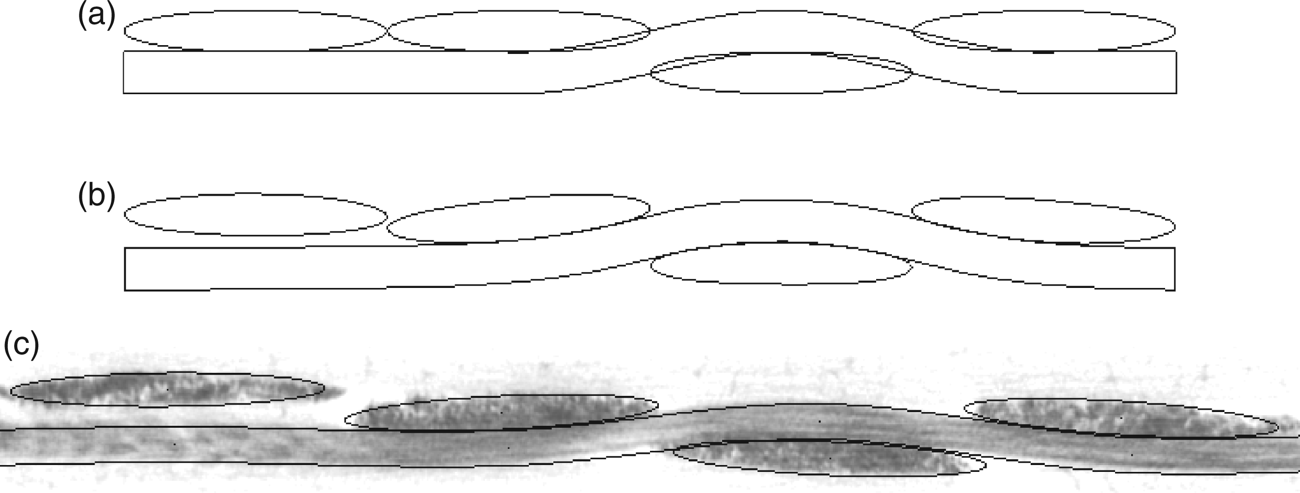

From these figures, it can be seen that geometry solver is able to predict the twist and position of the yarns for this fabric without the need for measured yarn mechanical property data. Specifically, it can be seen that the inter yarn penetration visible in Figure 12(a) between the longitudinally sectioned yarn and the rightmost three transversely-sectioned yarns is avoided by a combination of vertical translation and rotation of two of them, along with smoothing of the path of the longitudinally sectioned yarn to conform more closely with the lenticular cross-section of the yarns around which it deforms (Figure 12(b)). The resulting corrected shapes closely match the outlines visible in the Micro-CT image (Figure 12(c)). A clear contrast between initial and corrected yarn positions and shapes is also visible in Figure 13(a) and (b), along with good agreement between the latter and the Micro-CT measurements in Figure 13(c), though the mechanisms underlying these movements are less obvious as the contact zones are not visible.

Figure 13.

Chomarat 800S4-F1 cross-sections between yarns: (a) TexGen before, (b) TexGen after, and (c) Micro-CT.

3D orthogonal woven textile

A geometric model of a 3D orthogonal woven textile fabric (i.e., one involving multiple sets of stacked warp and fill yarns and an additional warp yarn running approximately perpendicular to act as a binder) was created in TexGen from the description given by Tan [28] (Table 3)^|| and the geometric solving method described above was applied. Figure 14 illustrates the fabric before and after solving with the default parameters. Due to the geometric complexity of the model, this took 50-minutes to solve over 18 iterations with a seed size of 0.5, 3609 nodes, and 5612 elements. A straightening of the weft yarns can be observed where the initial model contained excessive crimp. The path of the binder^¶ yarns have become smoother and the weft yarns twisted to accomodate this smoother path.

Figure 14.

3D orthogonal woven textile before and after geometry solving: (a) Before and (b) After.

Table 3.

Geometric properties of 3D woven textile

Yarn spacing (mm)	1.0
Yarn width (mm)	0.89
Yarn height (mm)	0.19
Fabric thickness (mm)	2.49

Micrograph comparison.

Figure 15 shows a comparison of predicted cross-sections taken along the center of a yarn with the corresponding micrographs.

Figure 15.

While the predicted and actual cross-sections do not show excellent agreement that was exhibited by the 2D test case, the mechanism in which the binder yarn path is smoothed by rotating the weft yarns is demonstrated both in the prediction and the micrograph. Intersections can be seen between the weft yarns similar to those seen in Figure 10(a); this spurious effect could be reduced by increasing the mesh density at the cost of increasing the computation time. The weft yarns on the opposite face to those directly rotated by the binders show much more rotation in the prediction than in the micrograph, suggesting that the twisting stiffness may be too large and may hence cause predicted bodily rotation of these yarns rather than local twisting to accommodate the binders.

This particular fabric illustrates the limitations of this technique. Throughout the derivation, a number of assumptions have been made which reduce its effectiveness for modeling fabrics with yarns, whose direction approaches the z-axis:

At the meshing stage, undesirable mesh distortions can occur. A high-quality mesh in 2D can become distorted when projected to the mid-surface of a yarn with a large slope. The element will be scaled in the direction of the slope by a factor of cos(θ)⁻¹, where θ is the slope angle.

In the element formulations, small slopes are assumed (i.e., sin θ ≈ θ) for reduced computation time and increased stability.

At the solving stage, the nodes do not have x- and y-displacement components and thus, displacements are restricted to the z-axis alone.

It is postulated that these limitations explain why the geometrical prediction for this 3D orthogonal weave is not as good as for the 2D weave.

Conclusions

A method for predicting the geometry of textile fabrics is presented using a FE technique. This article describes all the stages involved, including mesh generation, element formulation, contact algorithm, and solving. This has all been implemented in the TexGen software [20], providing an automated procedure.

Compared to analytical methods, this method is more generic and can be applied to different fabric architectures without modifications.

Compared to FE methods using volume elements, this method takes less computational time to solve and does not suffer from the inherent inability to accurately model the bending behavior of the discontinuous yarns using continuum elements.

Validation for two fabrics has been performed including a 2D weave and a 3D weave. Results for the 2D weave have been shown to compare very well to experimental data. Results for the 3D weave were predictably not so good due to the high level of crimp present in the binder yarn, but these were still an improvement over a purely geometric model.

Footnotes

†

These properties are typically difficult to obtain experimentally from single-yarn tests; so, assumed values must be generally used.

§

In this case, [T_t] = [T_t]^−T.

||

Due to problems with the slope of the binder yarn becoming too steep, the spacing between yarns was increased to 1.5 mm in TexGen where the binder yarns goes through the thickness of the fabric.

¶

The binder yarn is a yarn which keeps the layers in a 3D woven fabric together.

Acknowledgments

The authors gratefully acknowledge the support of EPSRC for this project via the Nottingham Innovative Manufacturing Research Centre, grant no. EP/E001904/1, and via the Platform Grant: Textile Composites - Engineering Science and its Applications, grant no. EP/F02911X/1. Some of the study contained in this article was originally presented verbally and electronically at a conference on 3D textiles [].

References

Zienkiewicz

Taylor

Zhu

. The finite element method: its basis and fundamentals, 6th edn. Amsterdam; Boston: Elsevier Butterworth-Heinemann, 2005.

Zienkiewicz

Taylor

. The finite element method for solid and structural mechanics, 6th edn. Amsterdam; Boston: Elsevier Butterworth-Heinemann, 2005.

Bathe

. Finite element procedures Englewood Cliffs, NJ: Prentice Hall, 1996.

Becker

. An introductory guide to finite element analysis Wiley/PE Publishing: Bury St Edmunds, UK, 2004.

Gallagher

. Finite element analysis fundamentals Englewood Cliffs, NJ: Prentice-Hall, 1975.

Boisse

Buet

Gasser

Launay

. Meso/macro-mechanical behavior of textile reinforcements for thin composites. Compos Sci Technol 2001; 61(3): 395–401.

Page

Wang

. Prediction of shear force using 3D non-linear FEM analyses for a plain weave carbon fabric in a bias extension state. Finite Elem Anal Des 2002; 38(8): 755–764.

Boisse

Zouari

Daniel

. Importance of in-plane shear rigidity in finite element analyses of woven fabric composite preforming. Composites Part A 2006; 37(12): 2201–2212.

Sherburn M. Geometric and mechanical modeling of textiles. PhD Thesis, University of Nottingham, July 2007.

10.

Badel

Vidal-Salle

Boisse

. Computational determination of in-plane shear mechanical behavior of textile composite reinforcements. Comput Mater Sci 2007; 40(4): 439–448.

11.

Lin

Sherburn

Crookston

Long

Clifford

Jones

. Finite element modeling of fabric compression. Model Simul Mater Sci Technol 2008; 16: 035010–035010.

12.

Sagar TV, Potluri P, and Hearle JWS. Energy approach to predict uniaxial/biaxial load-deformation of woven preforms. In: European Conference on Composite Materials 10 (ECCM-10), Brugge, Belgium, 3–7 June 2002.

13.

Sagar

Potluri

Hearle

JWS

. Meso-scale modeling of interlaced fiber assemblies using energy method. Comput Mater Sci 2003; 28(1): 49–62.

14.

Potluri

Parlak

Ramgulam

Sagar

. Analysis of tow deformations in textile preforms subjected to forming forces. Compos Sci Technol 2006; 66(2): 297–305.

15.

Glaessgen

Pastore

Griffin

Birger

. Geometrical and finite element modeling of textile composites. Composites Part B 1996; 27B(1): 43–50.

16.

Lomov

Huysmans

Luo

Parnas

Prodromou

Verpoest

Phelan

. Textile composites: Modeling strategies. Composites Part A 2001; 32A(10): 1379–1394.

17.

Hivet

Boisse

. Consistent 3D geometrical model of fabric elementary cell. Application to a meshing preprocessor for 3D finite element analysis. Finite Elem Anal Des 2005; 42(1): 25–49.

18.

Bogdanovich

Pastore

. Mechanics of textile and laminated composites London and New York: Chapman and Hall, 1996.

19.

Crookston

Long

Jones

. A summary review of mechanical properties prediction methods for textile reinforced polymer composites. Proc IMechE Part L: J Mater Des Appl 2005; 219(2): 91–109.

20.

Sherburn M. TexGen v3, tex.gen.sourceforge.net, (2007). Accessed on 13 September 2011.

21.

Shewchuk

. Delaunay refinement algorithms for triangular mesh generation. Comput Geom Theory Appl 2002; 22(1): 21–74.

22.

Shewchuk JR. Triangle: Engineering a 2D quality mesh generator and delaunay triangulator. In: Lin MC, Manocha D (eds)Applied computational geometry: towards geometric engineering, volume 1148 of Lecture Notes in Computer Science. Berlin: Springer-Verlagpp. 203–222, 1996 From the First ACM Workshop on Applied Computational Geometry. See also http://www.cs.cmu.edu/quake/triangle.html (accessed 15 March 2010).

23.

Harvey

Kelsey

. Triangular plate bending elements with enforced compatibility. AIAA J. 9(6): 1023–1026.

24.

Jones

. Mechanics of composite materials Washington, DC: Taylor & Francis Inc, 1998.

25.

PAFEC theory manual. Strelley Hall, Strelley, Nottingham: PAFEC Limited, 1984.

26.

Davis TA (ed.) Direct methods for sparse linear systems. Philadelphia: SIAM, 2006.

27.

Coxeter

HSM

. Introduction to geometry, 2nd edn. New York: Wiley, 1969.

28.

Tan

Tong

Steven

Ishikawa

. Behavior of 3D orthogonal woven CFRP composites. Part II: FEA and analytical modeling approaches. Composites Part A 2000; 31(3): 273–281.

29.

Sherburn M, Long A, Jones A. Prediction of textile geometry using strain energy minimisation. In 1st World Conference on 3D Fabrics and Their Applications (CD of short papers only, no printed or online proceedings). Manchester, UK, 2008.

Prediction of textile geometry using an energy minimization approach

Abstract

Keywords

Introduction

Initial geometric modeling and meshing

Identifying edges

Projecting edges

Identifying basic regions

Meshing basic regions

Creating mid-surfaces

FE formulations

Plate bending element

Plate tensile element

Contact algorithm

Boundary conditions

Solution method

Adjusting geometry

Yarn centerline

Yarn cross-section

Validation

Chomarat 800S4-F1

Mesh sensitivity.

Mechanical property sensitivity.

Micro-computed tomography comparison.

3D orthogonal woven textile

Micrograph comparison.

Conclusions

Footnotes

†

§

||

¶

Acknowledgments

References