Sage Journals: Discover world-class research

Abstract

In many problems from the field of textile engineering (e.g. fabric folding, motion of the sewing thread), it is necessary to investigate the motion of the objects in dynamic conditions, taking into consideration the influence of the forces of inertia and changing in the time boundary conditions. This article deals with the model analysis of the motion of the flat textile structure using Lagrange’s equations with constraints. The motion of the objects is under the influence of the gravity force. Lagrange’s equations have been used for discrete model of the structure. Numerical considerations presented in this article should give answer about practical usefulness of the Lagrange’s equations for solving the dynamic problem.

Keywords

textile mechanics elastica Lagrange’s equations equations of motion numerical methods

Introduction

Modelling and simulation of cloth deformation are of great importance in computer graphics and engineering applications. Although many models have been developed, problems still exist. No model so far can accurately describe both motion and deformation of cloth in a unified equation. And the equations for the in-plane deformation of cloth are yet to be developed. Cloth draping is of particular interest in the field of garment engineering. Most cloth draping simulation stresses the visual effects of garment design. However, the accuracy of the draping effect should not be overlooked, particularly for garment manufacturing. The accuracy of the draping behavior is largely affected by the fabric properties. Goldenthal [1], in his work, describes the dynamical behavior of textile structure using the Lagrange’s equations. In this work, the equations of motions are obtained from the Euler Lagrange equations. Next, he uses the Constrained Lagrangian Mechanics (CLM) framework to introduce constraints into the dynamic system. In order to do it, Lagrange multipliers have been introduced. Karthikeyan and Rnaganatan in their tutorial [2] on cloth modeling use the Lagrange’s equations of motion to describe the model of cloth. The Lagrange’s equations are fundamental equations of kinematics, which can be used to determine equilibrium position when the energy of a body is known.

Many textiles do not noticeably stretch under their own weight. Unfortunately, for better performance, many cloth solvers disregard this fact. Goldenthal and the others [3] propose a method to obtain very low strain along the warp and weft direction using CLM and a novel fast projection method. The numerical integration algorithm for constrained dynamics has been developed directly from the augmented Lagrange’s equation. The resulting algorithm acts as a velocity filter that easily integrates into existing simulation code. Au et al. [4] discuss the issue of incorporating the fabric properties into the cloth model, so that its raping behavior can be realistically simulated. These fabric properties are expressed in terms of a set of measurable mechanical properties. The draping behavior of the cloth is derived based on elastic theory. Dynamic draping simulation is presented with illustrative examples. You et al. [5] in their work describe a model for both motion and deformation of cloth, which will account for the in-plane deformation of cloth. In this model, the cloth deformations under out-plane and in-plane loads were uncoupled into out-plane and in-pane deformations. The theory of small deflection bending of plates with elastic behaviors was applied to the out-plane deformation and the theory of plane stress of elastic objects was applied to the in-plane deformation. Both static and dynamic problems of cloth were taken into account. The basic governing equations were given and the corresponding finite difference formulae were developed. The models developed from the energy minimization and finite element methods only considered the deformation of cloth. In the models developed from Lagrange’s equations of motion, both motion and deformation of the cloth are taken into account. Terzopoulos and Fleischer [6] proposed a deformable surface to model a piece of cloth based on Lagrange’s equation of motion. The derivation concentrated on the balance of forces: inertial force, damping force, other external forces, and the internal elastic and bending force acting on cloth.

In this article, only the theoretical considerations about using the Lagrange’s equations for simulation of motion of longitudinal section of textile were carried out.

In most cases of dynamic analysis of textile structures, it is necessary to use the model of heavy elastica, as a one-dimensional body of linear weight q and bending rigidity C in the state of large deflections. In this article, it is assumed that during the run of bending effect, the flat textile structure (e.g. fabric) will be represented as its longitudinal section. The mathematical model will be described as a flat deflection curve; this will be treated as a heavy elastica, as shown in Figure 1 and in ref. 7.

Figure 1.

The model of fabric approximate to elastic.

The word ‘heavy’ underlines the decisive influence of the gravity forces during the motion. It is assumed that the particular longitudinal sections do not act on each other by internal forces. Furthermore, the constancy of properties along the whole width of the bending strip is assumed. It will be assumed also that the elastica is inextensible. The analysis was made using Lagrange’s equations, describing the motion of the system of n particles in conservative force field. The variant of Lagrange’s equations with constraints was considered.

Discrete model of the object and the Lagrange’s equations

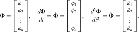
The Lagrange’s equations, describing the motion of the system of n particles in conservative force field, studying in detail among other things in the refs 8–11, are presented below

(1)

where T is kinetic energy, U is potential energy,

ϕ_{k}, {\overset{\cdot}{ϕ}}_{k}

are k-th generalized coordinate and velocity. If we have n generalized coordinates, then we can write n Lagrange’s equations (1).

The problem reduces to appropriate choosing of generalized coordinates $ϕ_{k}$ , deriving the formula for kinetic and potential energy, and next deriving and solving the Lagrange’s equations.

During the analysis, we often replace continuous systems by discrete systems using partition into n elements. In considered problem partition was made as follows.

The elastica of length L, mass M, and bending rigidity C fixed at point A was replaced by system of n masses of identical value $m = M / n$ , connected by n straight, inextensible and weightless segments of length $l = L / n$ , as shown in Figure 2 [12]. The other end B of elastica is free. If ρ is linear mass of elastica than $M = ρ L$ . The position of i-th mass is described by generalized coordinate as an inclination angle $ϕ_{i}$ $(i = 1, 2, \dots, n)$ of i-th segment to the vertical direction.

Figure 2.

Discrete model in coordinate system.

Coordinates of i-th mass and its derivatives are as below

(2)

The kinetic energy of i-th mass is $T_{i} = \frac{1}{2} m ({\overset{\cdot}{x}}_{i}^{2} + {\overset{\cdot}{y}}_{i}^{2})$ .

Therefore, the total kinetic energy of the system of n mass is

(3)

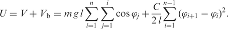
The total potential energy of the system U is the sum of the two components

(4)

where V is the potential energy of gravity forces and

V_{b}

is the potential energy of the bending.

The potential energy of gravity forces is $V = \sum_{i = 1}^{n} m g y_{i} = m g l \sum_{i = 1}^{n} \sum_{j = 1}^{i} \cos ϕ_{j}$ and the potential energy of the bending $V_{b} = \frac{1}{2} C \int_{0}^{L} {(\frac{d ϕ}{ds})}^{2} ds$ . After substitution of the derivative by difference quotient we have

(5)

Thus, the total potential energy of the system U is

(6)

The formula for derivative of kinetic energy T in respect of 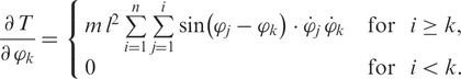$ϕ_{k}$ after transformations is as follows

(7)

After changing the limits of summation, we can write

(8)

Similarly, the other derivatives can be written as follows

(9)

(10)

(11)

The derivative 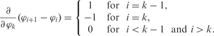$\partial (ϕ_{i + 1} - ϕ_{i}) / \partial ϕ_{k}$ depending on the value of index i is given by

(12)

Using summation from i = 1 to i = n – 1, the Equation (11) can be written as follows

(13)

Therefore, the derivative of total potential energy in respect of $ϕ_{k}$ is

(14)

Using the Equations (8), (9), and (14) in Lagrange’s equations (1), and dividing by 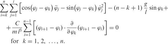$m l^{2}$ , we have

(15)

In this way, we get the system of n 2nd order ordinary differential equations with unknown variables $ϕ_{i}$ $(i = 1, 2, \dots, n)$ . Equation (15) represents k-th Lagrange’s equation, which describes the motion of elastica as in Figure 2.

Interpretation of boundary conditions results from formula for total potential energy of the system, as shown in Equation (6). In presented problem, the end B of elastica is free, therefore it is not loaded by any forces. The end A is fixed by joint, therefore the bending moment $M = 0$ , and displacements in point A are equal to zero (it has no influence on potential energy).

The Lagrange’s equations in the matrix form

For further analysis, the Lagrange’s equations (15) were written in the matrix form. The following denotations were introduced

In the matrix form, the Lagrange’s equations (15) are

(16)

where

A = A (Φ)

is an appropriate matrix and

B = B (Φ, \overset{\cdot}{Φ})

C = C (Φ)

and

D = D (Φ)

are vectors.

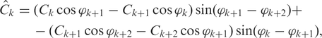
On the basis of the Equations (15), we can write the matrix A and vectors B, C, and D as follows

where the matrix S of dimension

n \times n

is defined by

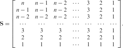
The element of k-th row and j-th column of matrix S can be written as

Its task is to realize the double summation from $i = k$ to $i = n$ and from $j = 1$ to $j = i$ .

Finally, it was obtained from system of n 2nd order ordinary differential equations with unknown generalized coordinates Φ in matrix form.

(17)

Numerical solution of the problem

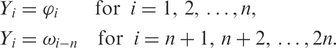
The system of Equation (17) we can write in the form of system 2n 1st order ordinary differential equations, introducing additional vector of generalized velocities $Φ = Ω = {[ω_{1} ω_{2} \dots ω_{n}]}^{T} .$ . In this way, we obtain

(18)

The system of Equation (18) has been solved using a standard Runge-Kutta-Fehlberg 4th order integration method. To solve this problem numerically, the following denotations were introduced

The vector of unknowns:

where

The right side of Equation (17) has been denoted by vector F, i.e.

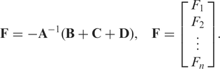
Finally, the following system of differential equations was solving

(19)

with initial conditions for

t = t_{0}

(20)

The Lagrange’s equations with two constraints

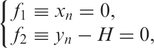
Previously the elastica fixed only at point A was considered. The other end B of elastica was free (Figure 2). In this case, generalized coordinates $ϕ_{k}$ were completely independent on themselves. In many problems connected with the motion of elastica, there are some constraints concerning angles $ϕ_{k}$ . Then the Lagrange’s equations undergo modification.

The motion of elastica with two ends fixed at two points A and B using joints as in Figure 3 will be considered. This case may be used for example to simulate fabric folding etc. Then, the boundary conditions for the end B (which previously was free) are as follows

Figure 3.

The elastica with two ends fixed at points A and B.

(21)

In accordance with Equation (2) for 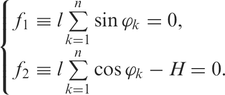$x_{n}$ and $y_{n}$ , we can rewrite the following two conditions of constraints (21), obtaining

(22)

Thus, the Lagrange’s equations we can write in the following form

(23)

where

λ_{1}, λ_{2}

are the unknown Lagrange’s multipliers (their interpretations are the appropriate reaction forces in point B - horizontal and vertical).

Derivatives $\partial f_{1} / \partial φ_{k}$ and $\partial f_{2} / \partial ϕ_{k}$ are as below

(24)

Let right side of the k-th Equation (15) be denoted by $Ψ_{k} (ϕ, \overset{\cdot}{ϕ})$ . Therefore, using (23) and (24), we have the following system of equations

(25)

Using matrix notation, we can write new matrix form of the system (25)

(26)

where

The system of Equation (26) with the Equations (22) presents the system of n + 2 differential-algebraic equations with n + 2 unknowns, that is: n generalized coordinates $ϕ_{i}$ $(i = 1, 2, \dots, n)$ and two Lagrange’s multipliers $λ_{1}, λ_{2}$ . To solve such problem, the Equations (22) has been differentiated two times in respect of time

(27)

Next from Equations (26), the multipliers $λ_{1}$ and $λ_{2}$ have been eliminated successively, using twice Gaussian elimination. After this, Equations (26) together with (27) present the system of n 2nd order ordinary differential equations in respect of $ϕ_{i}$ $(i = 1, \dots n)$ . Using matrix notation, we have

(28)

similarly as (16). The components of new matrix

\overset{\land}{A}

and vectors

\overset{\land}{B} \overset{\land}{C} i \overset{\land}{D}

are as below For

k = \dots n - 2

and

The system of Equations (28) has been transformed to the form

(29)

Next, we can write

(30)

Finally, the system of Equations (30) has been solved using a standard Runge-Kutta-Fehlberg 4th order integration method.

The considerations presented above are concerned with the elastica for which the end B was fixed by joint. Of course, the other conditions of constraints may be introduced for this one.

If we want to allow vertical motion of the end B, then we have only one constraint for coordinate x of the end B: x must be always equal to value $a = const.$ and we have only one algebraic equation (conditions of constraints) in the form of $f_{1} \equiv x_{n} - a = 0 .$

The Lagrange’s equations are simple in this case because we have only one Lagrange’s multipliers $λ_{1}$ .

If we want to have the end B fixed at point B at an angle of $ϕ = α$ , where $x = a$ , $y = b$ , then there are three conditions of constraints

and three Lagrange’s multipliers

λ_{1} λ_{2} λ_{3}

The results of calculations

To present the results of calculations and accuracy of numerical method, two numerical cases were considered.

The first case concerns the problem of motion of heavy elastica under the influence of gravity force. The elastica is fixed at one end only, as shown in Figure 2.

The second case concerns the problem of motion of elastica fixed at two ends, as shown in Figure 3.

The motion of the elastica fixed at one point

In this case, the elastica fixed at one point by joint as in Figure 2 will be considered. The second end is free. The motion is under the influence of the gravity and elastic forces.

The properties of the elastica are as follows:

– bending rigidity C = 0.0025 ${Nm}^{2}$

– linear mass density ρ = 0.01 kg/m,

– length L = 1 m.

To many points n of division can affect to long time of calculations. In the example below, it has been assumed that n = 8.

The initial conditions (20) are as follows

In the initial instant, the elastica has rectilinear, horizontal shape. The velocity of all points is zero. After solving the Equations (18) with the time step $Δ t$ = 0.005 s, it has obtained the shape of elastica in the following time instant $t_{0} t_{1} t_{2} \dots$ The shapes are presented in Figure 4. Figure 5 shows variations of generalized coordinates $ϕ_{1} ϕ_{2} \dots ϕ_{8}$ in the respect of time t. Figure 6 shows variations of generalized coordinates $ϕ_{1} ϕ_{2} \dots ϕ_{8}$ in the respect of time t for elastica of bending rigidity 10 times less than before (C = 0.00025 ${Nm}^{2}$ ).

Figure 6.

The variation of generalized coordinates $ϕ_{1} ϕ_{2},\dots, ϕ_{8}$ in the respect of time t for bending rigidity of C = 0.00025 ${Nm}^{2}$ .

Figure 5.

The variation of generalized coordinates $ϕ_{1} ϕ_{2},\dots, ϕ_{8}$ in the respect of time t.

Figure 4.

The shape of elastica in the following time instant from $t_{0}$ to $t_{20}$ .

In the Figures 5 and 6, the heavy dashed line represents graph of angular displacement of rigid rod (physical pendulum) fixed in the same point as elastica (Figure 7).

Figure 7.

The rigid rod as physical pendulum.

From the graphs it may be inferred that in the initial state of the motion, the points of elastica oscillate around the dynamic equilibrium (as for physical pendulum). The rigid rod (Figure 7) can be treated as the elastica of bending rigidity $C = \infty$ for which all points have permanently the same angular displacements $φ_{k} = φ dla k = 1, 2, \dots, n$ . As time goes, deviations from dynamic equilibrium become bigger and bigger.

In order to check accuracy of calculations, we follow as below.

For chosen coordinate $ϕ_{8}$ its values marked by $ϕ_{8}^{Δ t_{1}}$ with given time step $Δ t_{1}$ = 0.005 s have been calculated. Next, the calculations have been repeated for the less time step $Δ t_{2}$ = $1 / 2 Δ t_{1}$ . The difference $Δ ϕ_{8} = ϕ_{8}^{Δ t_{1}} - ϕ_{8}^{Δ t_{2}}$ has been determined for following $t_{i} = t_{0} + i \cdot Δ t_{1}$ .

The calculations have been made for C = 0.0025 ${Nm}^{2}$ . The graph of differences $Δ ϕ_{8}$ for following time instant is presented in Figure 8.

Figure 8.

Test of accuracy of generalized coordinate $ϕ_{8}$ in the following time instant.

The differences $Δ ϕ_{8}$ are not big at all (between −0.00019 and 0.00022 rad), even after large number of iterations (i = 400). The accuracy turned out to be satisfactory.

The motion of the elastica fixed at two points

In this case, the elastica fixed at two points by joints as in Figure 3 will be considered. The motion is under the influence of the gravity and elastic forces.

The properties of the elastica are as follows:

– bending rigidity C = 0.0015 ${Nm}^{2}$

– linear mass density ρ = 0.01 kg/m,

– length L = 1.2 m.

Number of points of division is n = 16. The system of equations (30) has been solved using Runge-Kutta-Fehlberg 4th order integration method with time step $Δ t$ = 0.005 s. The initial conditions (20) are as follows

Finally, the shape of the elastica in the following time instant $t_{i}$ has been obtained. It is presents in Figure 9.

Figure 9.

The shape of the elastica in the following time instant.

In order to check accuracy of calculations, we tested how the boundary conditions (21) change as time goes by. In this way, we can check how the algorithm secures fulfillment of the boundary conditions

As a measure of deviation of boundary conditions, we can take $Σ = | f_{1} | + | f_{2} |$ , which, if the boundary conditions are fulfilled, should be equal to zero. The calculations have been made for two time steps: $Δ t_{1}$ = 0.005 s i $Δ t_{2} = 1 / 2 Δ t_{1}$ . The variation of Σ in respect of number of iterations are presented in Figure 10 for two time steps.

Figure 10.

The analysis of fulfillment of the boundary conditions $Σ = | f_{1} | + | f_{2} |$ .

From the Figure 10, we can conclude that for two times less time step deviation of boundary conditions was significantly less. For $Δ t_{1}$ after 300 iterations deviation was about $2 \cdot 10^{- 4} m$ , and for $Δ t_{2} = 1 . / 2 Δ t_{1}$ deviation was about $2 \cdot 10^{- 5}$ (10 times less).

Conclusion

After carrying out series of numerical tests it can be concluded that Lagrange’s equations are practically useful for the analysis of the motion of heavy elastica. This is one way to solve the problem presented in this article. The Lagrange’s equations are the tool to get the solutions. In this case, the Lagrange’s equations are useful. The speed of calculations and time to get results are satisfying. Of course, the other methods may be useful as well. The intention of the author of this article was only using of Lagrange’s equations.

The method can be used for simulation of many problems from the field of textile mechanics, for example fabric folding (Figure 11), motion of the sewing thread etc. Similar investigations, but not using Lagrange’s equations, have been described by Lloyd [13].

Figure 11.

The simulation of fabric folding using Lagrange’s equations.

The results of calculations show clearly wave nature of phenomenon. The bending rigidity has no influence on the convergence of the results. The analyzed motion of elastica is stable owing to initial conditions. The applications field of Lagrange’s equations is not closed yet. In the future works, the method presented in this article will be applied for simulation of new test of bending length based on fabric folding. Numerical simulation should give answer about practical usefulness of this test.

Footnotes

Notes

Piotr Szablewski is a Senior Lecturer at the Department of Technical Mechanics and Informatics, Technical University of łódź, Poland. He did his MSc in 1987 (Thesis: Kinematic and Dynamic Analysis of Choosen Elements of Rapier Loom KR8A) and PhD in 1997 (Dissertation: Modelling of Cylindrical Bending of Textile Structures). He worked as Teaching Assistant during 1987–1997, Lecturer, 1997–1998, Senior Lecturer, since 1998. He has over 18 years experience in the teaching of mechanics and numerical methods in engineering. He is interested in the theoretical methods and numerical simulation. Especially, he is interested in theoretical mechanics and its applications in textiles. Besides, he is interested in strength of materials and computer-aided engineering calculations. During the last three years he has been working on applications of numerical methods for building geometrical models of textile composites and predicting mechanical parameters. He has also experience in working with international students group in the area of mechanics (European Project Semester in 2005).

References

Goldenthal AR. Implicit treatment of constraints for cloth simulation, PhD Thesis, The Hebrew University of Jerusalem, March 2010.

Karthikeyan PS and Rnaganatan PS. Tutorial on cloth modelling, http://br.reocities.com/SiliconValley/heights/5445/cloth.html (last updated May 2, 1998).

Goldenthal

Harmon

Fattal

Bercovier

Grinspun

. Efficient simulation of inextensible cloth. ACM Transactions on Graphics 2007; 26: 49–55.

Au CK, Wu Z and Yuen MMF Effect of fabric properties on cloth draping modeling, geometric modeling and processing 2000, 10–12 April 2000, Hong Kong, China, pp. 69–76.

You

Zhang

Comninos

. Cloth deformation modelling using a plate bending model, The 7-th International Conference in Central Europe on Computer Graphics, Visualization and Interactive Digital Media, 9–12 February 1999, University of West Bohemia, Pilsen, Czech Republic, pp. 485–491.

Teropoulos

Fleischer

. Deformable models. Visual Comp 1988; 4: 306–331.

Szablewski

Kobza

. Numerical analysis of Peirce’s Cantilever Test for the bending rigidity of textiles. Fibres & Textiles in Eastern Europe 2003; 4: 43: 54–57.

Leyko J. Dynamika ukladów materialnych, cz. II, PWN, Warszawa, 1961.

Greiner

. Classical mechanics: Systems of particles and hamiltonian dynamics. New York: Springer Verlag New York, Inc, 2003.

10.

O'Reilly

. Intermediate dynamics for engineers: A unified treatment of Newton Euler and Lagrangian Mechanics. New York: Cambridge University Press, 2008.

11.

Taylor

. Classical mechanics, California: University Science Books, Mill Valley, 2005.

12.

Szablewski P. Modelling of dynamical behaviour of flat textile structure using Lagrange’s equations, In X International Conference IMTEX 2009, Łódz, 2009, pp. 35–38.

13.

Lloyd

Shanahan

Konopasek

. The folding of heavy fabric sheets. Int J Mech Sci 1978; 20: 521–527.

Lagrange’s equations with constraints in model applications from the field of textile mechanics

Abstract

Keywords

Introduction

Discrete model of the object and the Lagrange’s equations

The Lagrange’s equations in the matrix form

Numerical solution of the problem

The Lagrange’s equations with two constraints

The results of calculations

The motion of the elastica fixed at one point

The motion of the elastica fixed at two points

Conclusion

Footnotes

Notes

References