Exploring the latent space distribution of a graph autoencoder trained on 3D models of modernist architecture

Abstract

Building on previous research in generative graph machine learning in architecture, this paper investigates how data generation and preparation can change the distribution of a model’s latent space and thus its generative qualities. Therefore, we first present and discuss our previous approach of applying generative graph machine learning in architecture by sampling the latent space of a graph autoencoder trained with the augmentations of four examples of modernist buildings. We then present a new method of data generation for modernist buildings in the style of architect Mies van der Rohe, which produces a large range of 3D building models with great geometric variety. Trained on the new dataset, the graph autoencoder shows a more continuous latent space, confirmed by visual comparison and by three spatial analysis algorithms that quantitatively assess the spatial structure of the different latent spaces.

Introduction

Here we present an extended and improved version of the graph-based generation method of 3d architectural models presented originally in Bauscher et al. ¹ The original paper presents a generative AI system that outputs new spatial configurations of architectural elements in three dimensions. The graph-based autoencoder can read 3d buildings as training input and does not rely on any sort of conversion between 2d images or plans and a desired three-dimensional output in post. It presents a very intuitive approach to generate 3d models for architects, which although only simple, already shows some understanding of important architectural features that are used in generation. That makes it very well rooted in the modern idea of the architectural design process. In the following, we discuss and improve its method of data generation to further elevate performance and its raison d’être.

State of the art

Current research in generative AI in architecture can be divided into 2D generative models based on images or vector graphics (photographs/floor plans/sections), and 3d generative models based on stacked images, point clouds, voxel- or mesh geometries or BIM data. 2D image generation has successfully been used the longest, due to its great accessibility and generalizability towards architecture. In addition, it offers an almost seamless integration into the contemporary workflow of architectural design, requiring a minimum of postprocessing before the result is fully usable (i.e., if anything, a quick AI-based visualisation of a design idea only needs to be edited in Photoshop to be presentable as the designer’s idea). No special research for the architectural domain was necessary, but architects can use state-of-the-art models like DALL-E ² and Stable Diffusion. ³ Only some big architecture offices like Zaha Hadid Architects and Coop Himmelb(l)au developed their own, in-house models to be able to further control the output.

In contrast, 3D and geometry-based generative models do always need to be specifically developed or at least adjusted for architectural application thus are less mature and harder to be directly applied to the architectural design process without any manual postprocessing. In addition, “[…] personal barriers often restrict their [the architects’] access to the latest technological developments, thereby causing the application of generative AI in architectural design to lag behind”. ⁴ Other challenges include “[…] computational overhead, training stability, and the limited availability of high-quality 3D datasets.” ⁵

Most successful methods of encoding and generating 3d building information rely at least partially on 2d information. That could be floor plans, sections and depth information from which a 3d model is generated.^6,7 Other models rely on fully 3d based information, either encoding voxel data,^8,9 point clouds, ¹⁰ or Bim data, ¹¹ which all have improved in realism and logic recently but still tend to generate rather conceptual 3d models in need of at least some postprocessing or manual intervention for further use.

Graphs

Graph representations of buildings or parts of buildings have been used for a long time in architecture, ¹² mainly due to their shared property of being non-discursive, meaning they cannot be fully described by words or rules. ¹³ In comparison to other data formats that can be used to train any machine learning model, graphs have the advantage of being able to store information about multiple types of data as well as information about relationships. ¹⁴ This focuses the attention of the model on the logical and geometrical properties of buildings, rather than on the visual appearance.

Original methodology

Dataset

The custom dataset used previously consists of four modernist buildings that have been individually remodeled parametrically in Grasshopper inside Rhino. That gave the opportunity to easily augment each building in its geometry to create more data for training the autoencoder. All houses are from the same architectural period, modernism, for the ease of remodelling and a geometric continuity across all data. The buildings are Mies van der Rohe’s Barcelona Pavilion (1929), Ray and Charles Eames’ Eames House (1949), Mies van der Rohe’s Farnsworth House (1951) and Pierre Koenig’s Stahl House (1960).

Those houses all follow the design principle of only using orthogonal walls, as well as mostly having full-height openings for windows. Yet they vary greatly in size, proportion and location.

To avoid overcomplication in the 3d model, the buildings were remodelled as a surface model. Meaning walls, floors and ceilings are all seen as individual, rectangular surfaces without any thickness, while doors and openable windows are just empty spaces. This supports the idea of trying to model space-defining elements only, so there is no need for i.e., any structural considerations.

This approach fails in providing the autoencoder with a heterogeneous dataset, mainly due to the method of augmentation. Starting always from the original model, elements are only slightly moved and scaled randomly in one direction (Figure 1), creating not enough variation to allow for a smooth geometrical translation between the original buildings. The augmentations still always keep the same layout, element count, division between horizontal and vertical elements, overall size and ratio. Thus, also the graph structure does not change between augmentations.

Figure 1.

The previous method of geometry augmentation in plan, blue highlights the parametric parameters.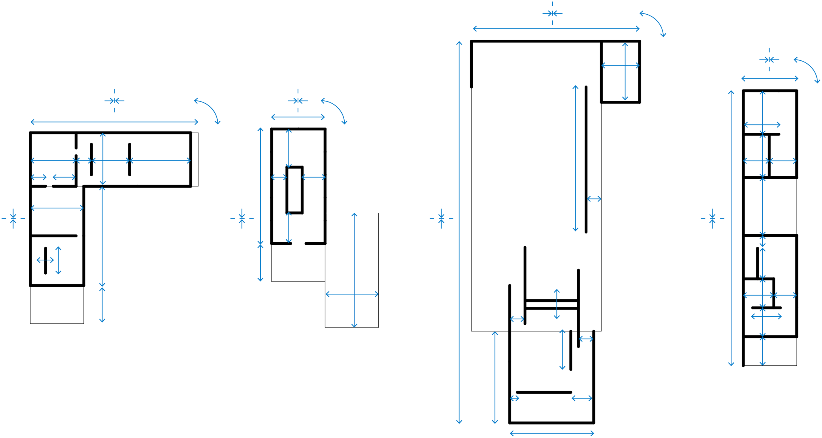

In addition, the augmented geometries are randomly rotated around their central Z axis in increments of 90°, as well as randomly mirrored in X and Y directions. On one hand, this creates a more diversified and interesting space for generation, on the other hand, it introduces unnecessary noise into the latent space and thus makes the results harder to read and understand.

Data representation

Each surface-based 3d building model in the dataset is translated into an undirected graph, where all geometrical information is held in the node features. Each node represents one surface, and nodes are connected in the graph if they physically touch in the 3d model (Figure 2). To encode all necessary information, the node features contain the coordinates of the centre point, the orientation and the width and length of the surface. Here we must point out that this specific method of conversion only allows for orthogonally positioned elements. The orientation value equals one of the three global planes (XY, XZ, YZ) and thus limits the geometrical options for input and output. This method of representation proved to be in line with the geometrical idea of modernist architecture and is also used in the here presented research.

Figure 2.

Previously and currently used graph representation of a surface-based 3D model.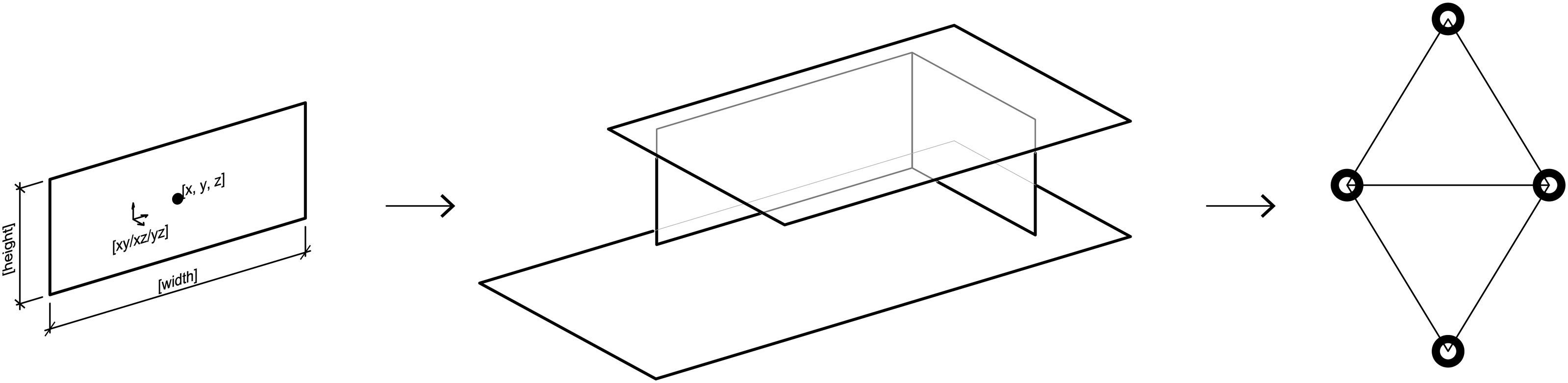

Graph autoencoder

The graph autoencoder model (Figure 3) is defined by the encoder and decoder models. Here, the encoder is graph-based as first described by Kipf and Welling ¹⁵ consisting of message-passing layers, ¹⁶ while the decoder consists of linear layers that do not create or use any graph structure. That means all input data must have the same count of elements because reconstructing the features through linear layers flattens the data into a one-dimensional vector with always the same length. Another limitation is the chosen dimension of the latent space - three - which restricts the performance of the model. This was chosen for easy visualisation considering the model itself might be the least deciding factor on the performance of the whole system, but data collection and preparation are far more important. ¹⁷

Figure 3.

Previously used graph autoencoder model.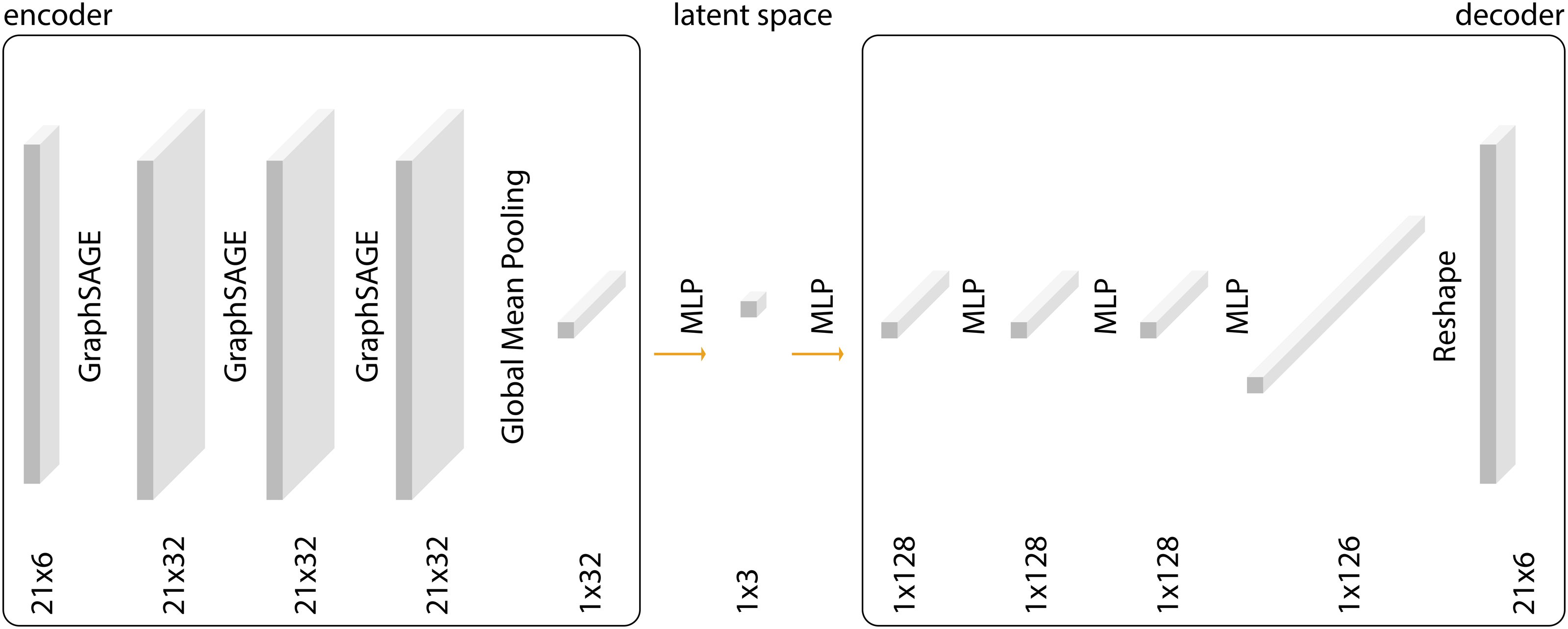

Adapted methodology

Dataset

Aroyo et al. ¹⁸ point out: “Data is potentially the most under-valued and de-glamorized aspect of today’s AI ecosystem” and “Benchmark datasets are often missing much of the natural ambiguity of the real world”. Both points can be applied to our previous research on generative graph autoencoders in architecture. The second point is harder to approach due to the limited number of three-dimensional datasets of buildings ready to use. The usage of a 2d-floor plan dataset as they are widely available^19–21 seems to not only defeat the conceptual idea of the research project but also still poses multiple questions on the quality and origin of the data.

Therefore, we propose further developing the existing dataset towards a more heterogeneous geometrical landscape for better overall performance. Instead of using the original geometries of precedent buildings as a starting point for simple geometric augmentation, we now use an iterative algorithm that applies predefined geometric rules for generating the dataset. We use three buildings as concrete inspiration for deriving the mentioned rules, Mies van der Rohe’s Farnsworth House (1951), Barcelona Pavillon (1929), and the conceptional plans drawn around 1923 for the Brick Country House (Figure 4). By choosing architectures by the same architect as guidelines, which differ in size, typology, proportion, and layout but follow similar geometrical design principles (open floor plan, grids, horizontal planes), we open the room for a more seamless transition between the geometries in the new dataset (Figure 5).

Figure 4.

Plans Mies van der Rohe. Left: Farnsworth House, Centre: Barcelona Pavillon, Right: Brick Country House. Original plans simplified and redrawn by the author.

Figure 5.

Examples of the new dataset in the style of Mies van der Rohe.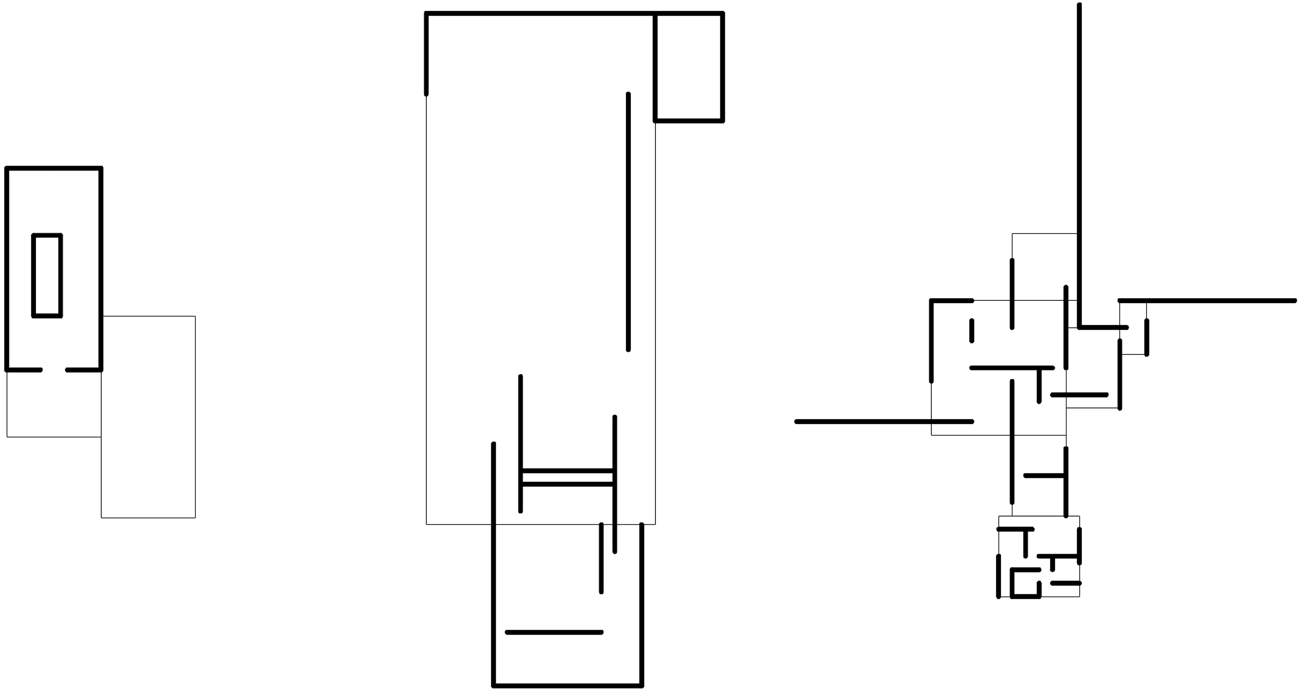

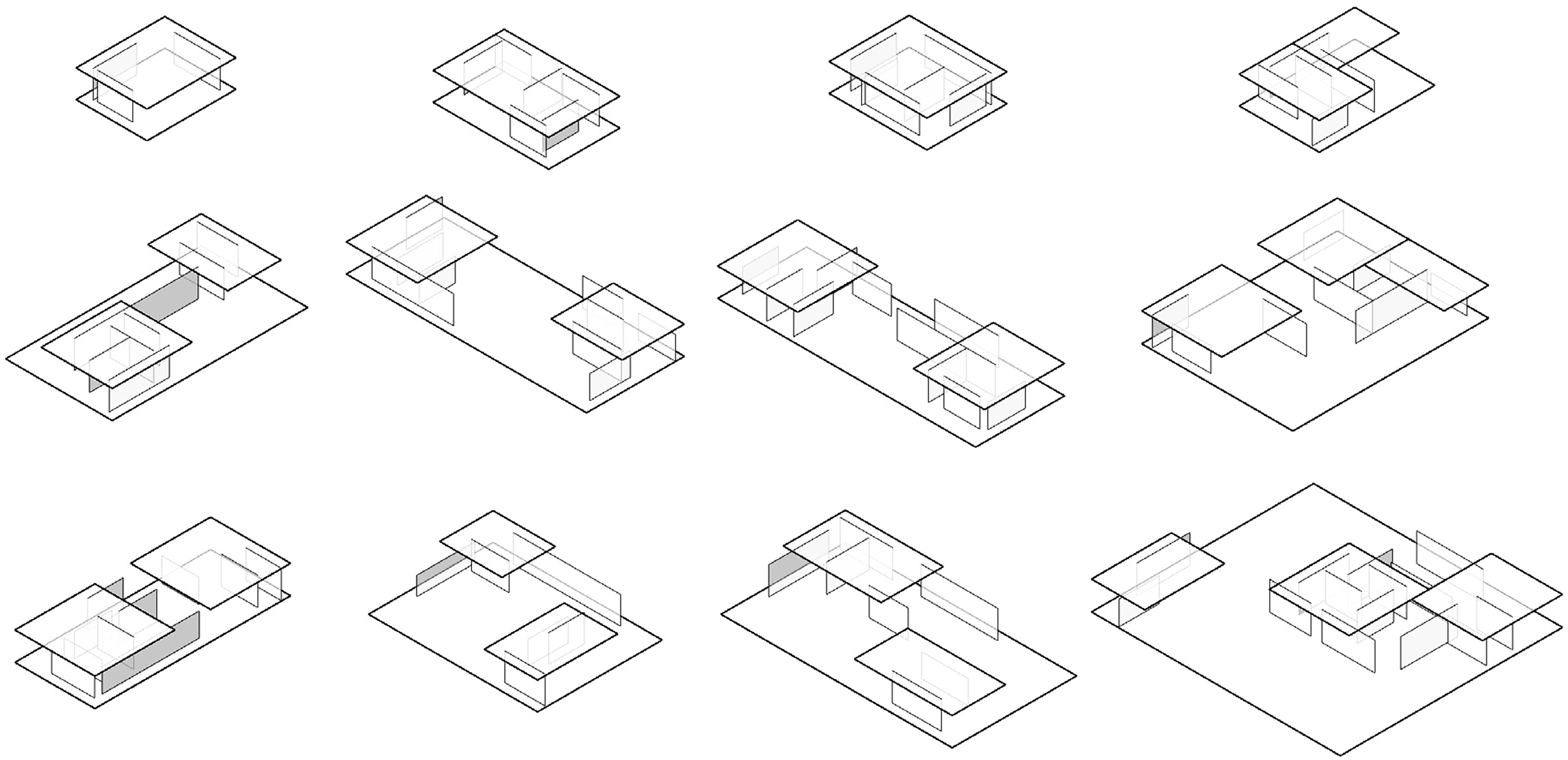
For the parametric generation, the original dimensions and ratios of geometric elements in the three houses as well as standard architectural principles were combined with some randomness. In addition, non-geometrical parameters were set by us, taking over a higher-level designer role and ensuring the spatial qualities and logic of the generated models.

As a main driver for the definition of space in Mies van der Rohe’s geometries, we identified the roof shapes. Rectangles with similar dimensions and offsets as the original houses are initially placed in the generative algorithm (Figure 6), which is implemented in the Grasshopper/Rhino environment. These roof rectangles are then further subdivided into the subspaces over which they lie. In the example buildings, Van der Rohe never designed a room fully enclosed with walls and accessible by a door (other than the washrooms and storage), but rather focused on the openness and fluidity of space. We try to emulate this method of design by iterating through each individual edge of each subspace, and having the algorithm take the decision of either placing a wall of a certain length at the current edge or keeping the space open based on decision values manually set by us as designers. Finally, a floor geometry is generated by creating a boundary rectangle around the wall and roof projections.

Figure 6.

Schematic diagram of the algorithm to generate the dataset.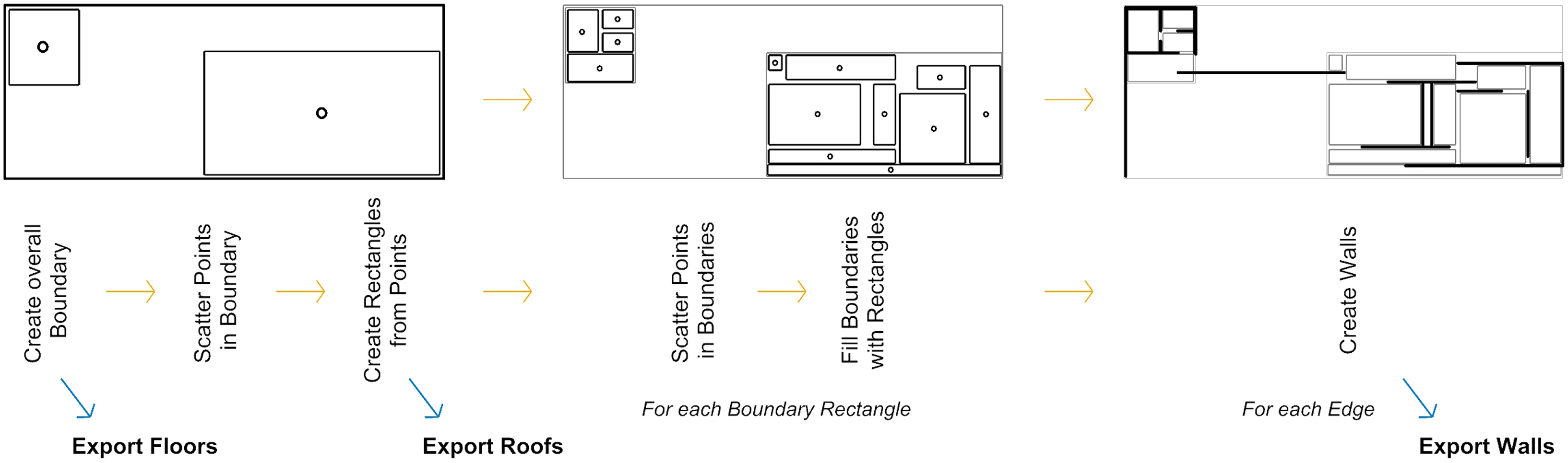

Graph autoencoder

The graph autoencoder model (Figure 7) stays mostly the same as described in the original methodology section, with the only change that it now can handle graphs of different sizes. It takes as input a set of node features (N_max × 6), where each node is represented by a vector of six values encoding the 3d geometry (Figure 2). N_max denotes the maximum number of nodes across all training samples. For graphs with fewer N_max nodes, zero-padding is applied to ensure consistent input size across the dataset.

Figure 7.

Graph autoencoder model with variable node count in training data.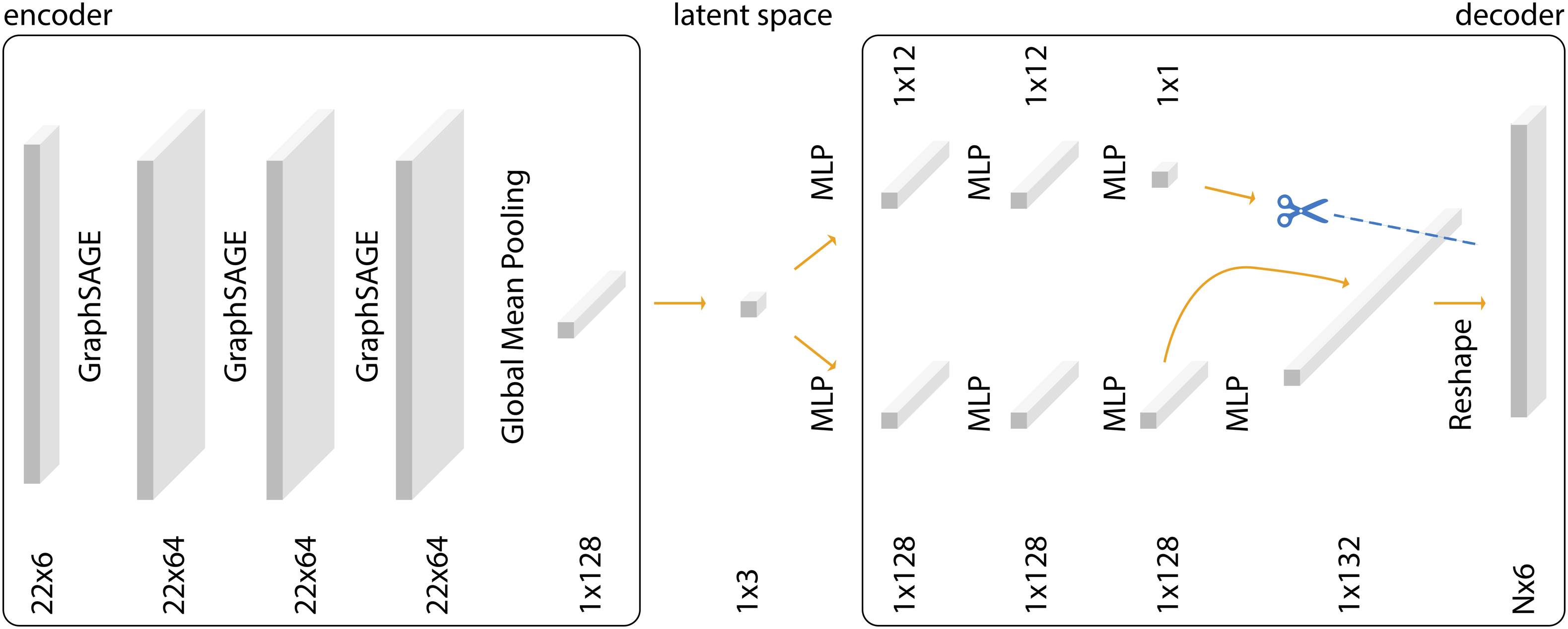

The encoder uses graph-based message passing to capture both local and global structural information. The resulting graph representation is then flattened into a one-dimensional latent vector. This vector is passed through a series of fully connected layers in the decoder, which reconstructs the padded node feature set of size N_max × 6. The model is always trained using a loss computed over this fully padded, generated output.

In the decoder, we train a lightweight auxiliary model in parallel consisting of two fully connected layers, which takes the latent representation as input and predicts the actual number of valid (non-padded) nodes in the original graph. This two-branch approach allows the network to handle variable-sized graphs while maintaining a fixed-dimensional latent space, aligning with recent findings on learning with variable-length structured data. ²²

The final model used the following variables:

- Epochs: 1000

- Learning Rate: 0.001

- Optimiser: Adam

- Loss function: Mean Squared Error

- Activation function: ReLu

- Train, Validate, Test: 80%, 10%, 10%

Results

We compare the newly trained and improved latent space with the previously used latent space as well as a reference set of points generated via the Sobol sequence, which serves as an optimal reference for well-distributed points (Figure 8). The points in both trained latent spaces represent the latent mapping of the dataset buildings by the respective trained autoencoder. The Sobol sequence is used for its quasi-random properties, ensuring points are evenly distributed across the space, ²³ which makes it an ideal comparison for evaluating the distribution qualities of latent spaces.

Figure 8.

Visual comparison of latent spaces, left: previous research, centre: new research, 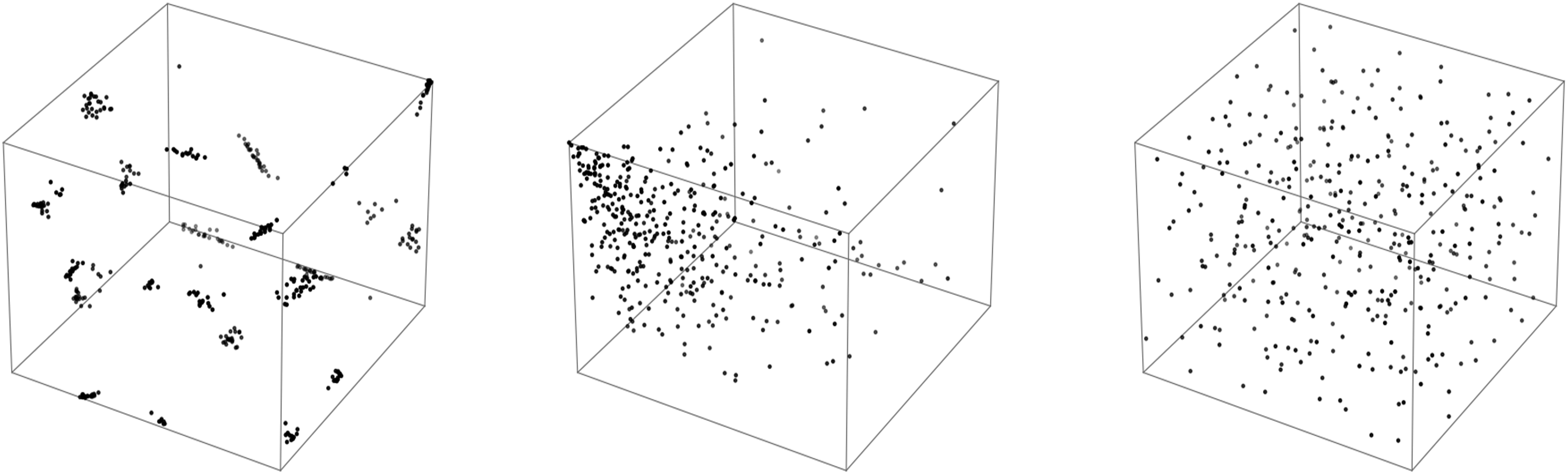right: Sobol points.

Apart from a visual comparison (Figure 8), we use three algorithms (Tab. 1), that quantitatively assess the spatial structure of our data, analysing the distribution, density, and clustering of points in a 1³ cube: average nearest neighbor distance, DBSCAN clustering, and kernel density discrepancy. The first method, average nearest neighbor distance, is widely used in spatial analysis and measures the mean distance between each point and its nearest neighbor, providing insight into the overall distribution of points. ²⁴ DBSCAN, a popular density-based clustering algorithm, identifies clusters by grouping points based on their density. ²⁵ Lastly, the kernel density discrepancy measures the variation in point density across a 3D grid and helps assess the evenness of point distribution in the latent space. ²⁶

Table 1.

Quantitively comparison of latent spaces.

Dataset	Average nearest neighbor distances (higher is better)	DBSCAN (clusters, noise, points) (lower is better)	Kernel density discrepancy (higher is better)
Previous latent space	0.0161	23 clusters, 7 noise points	102.4063
New latent space	0.0553	3 clusters, 112 noise points	117.9843
Sobol points	0.0960	1 clusters, 395 noise points	125.3987

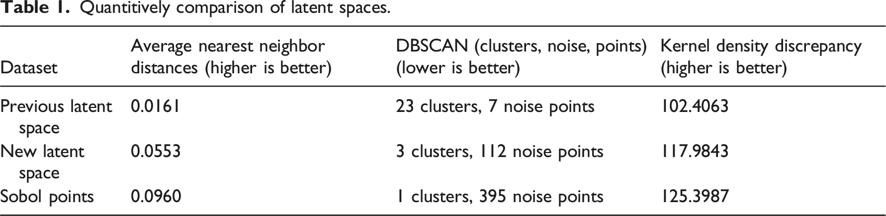
The comparison of values across the three latent spaces aligns well with their visual structures. The new latent space, trained with an improved dataset, shows a noticeable improvement over the old latent space in kernel density discrepancy, nearest neighbor distances and amount of clustering, reflecting a more uniform distribution and proving the value of good data preparation. However, it still falls short when compared to the Sobol points, which, as expected, provide the best results in terms of even distribution and low clustering due to their quasi-random nature. Nevertheless, the new latent space performs significantly better than the old one, which had a higher clustering tendency and less uniform density, proving a promising improvement for future applications in sampling and interpolating building models from the latent space.

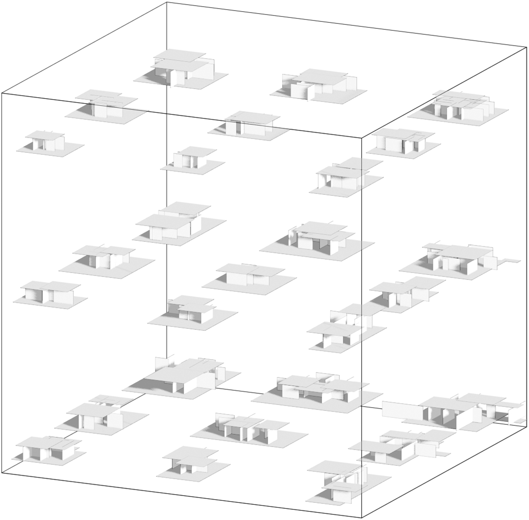
The new latent space also demonstrates a structured and meaningful distribution of the dataset, suggesting that the model has effectively learned a representation mainly based on geometric logic thanks to the new method of generation. When visualized with points coloured according to the total area and total count of surfaces in the training geometries (Figure 9), a smooth transition from high to low values is shown across the latent space. Similarly, this can be observed when sampling a grid of unknown points in the latent space (Figure 10), where the geometry in the bottom right corner has the highest surface count and -area, while the top left has the lowest. This continuity indicates that the model is organizing data points in a way that preserves meaningful spatial and geometric relationships, rather than scattering them randomly or basing the distribution on a poorly augmented and prepared dataset as before. This structured latent space provides a strong foundation, offering a higher chance of generating spatially and geometrically coherent 3d models when sampling new points in the latent space. In contrast to an unstructured or clustered space, this allows for more predictable and interpretable interpolations in the generated geometries, improving the overall reliability of the trained autoencoder.

Figure 9.

Distribution of dataset in latent space, coloured according to total amount of elements (left) and total area (right). Both times blue represents the smallest quantities of elements and red the largest.

Figure 10.

Sampling of unknown points in the latent space.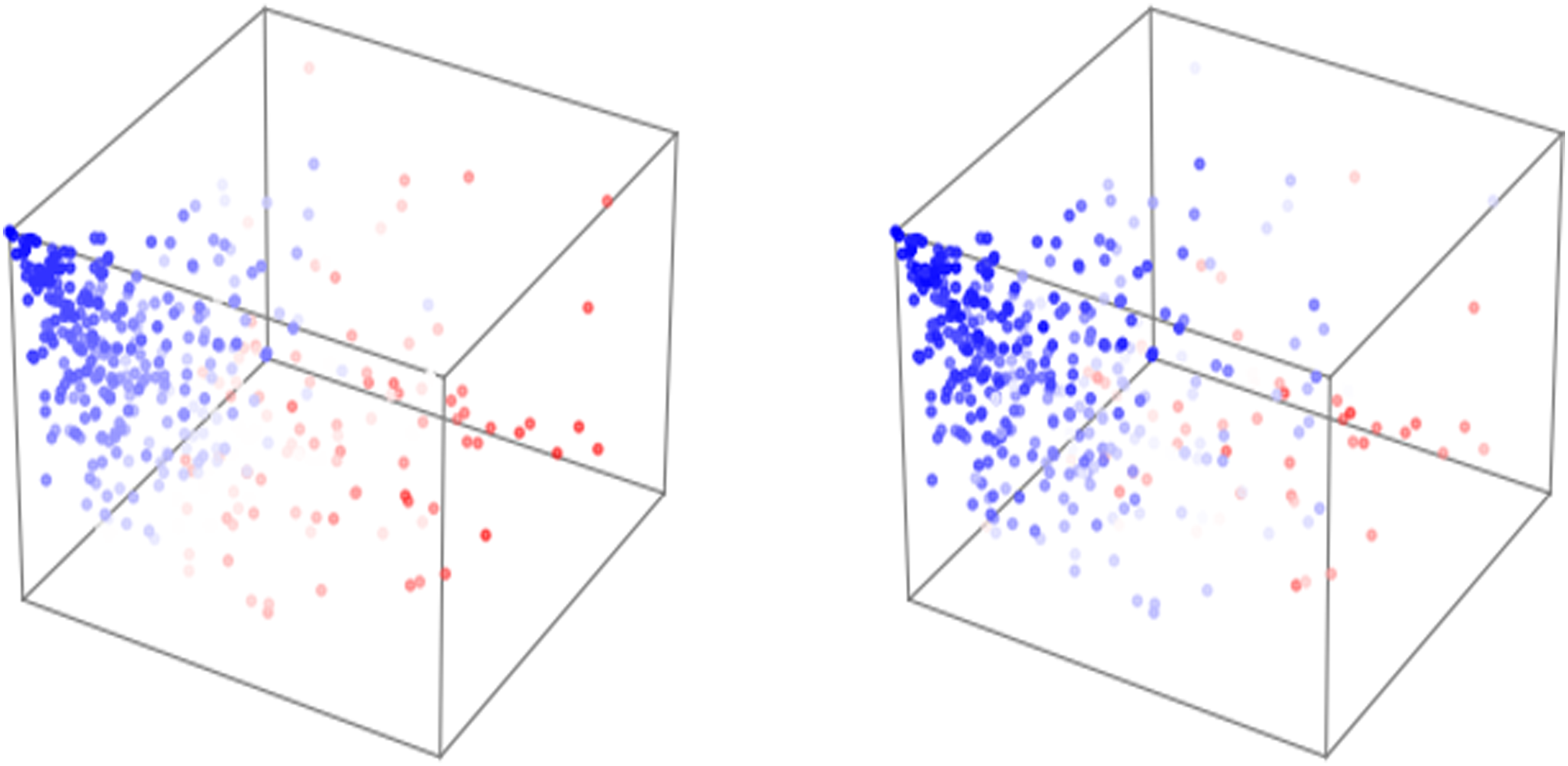

Discussion

This research highlights the importance of data preparation, showing the successful implementation of a new augmentation method for 3d architecture datasets based on a limited number of existing architectural designs.

While the deterministic algorithm for generation already provides us with new geometries that follow our rules set to create “Miesian” 3d models, we argue that using a generative autoencoder gives us multiple advantages: (1) It can adapt to large or different datasets, while a deterministic model would need to be rewritten to fit any other use case. (2) It offers a smooth interpolation between known designs, which can lead to unexpected new forms and spaces. The deterministic model is not able to create any interpolated geometry. (3) More parameters can be included in the future. The model can be trained to prefer optimized designs, and the generative process does not solely need to be based on the intuitive navigation of the latent space by a designer.

The next steps could include: (1) Further testing and optimization of the model to evaluate its new generative capabilities, including a direct geometrical comparison of the generated 3d models using methods such as the average Hausdorff Distance, both between datasets and against real-world spatial data. This would provide a more geometrically grounded verification of the distribution quality and heterogeneity achieved through the new generation method. (2) Redesigning the model to be either a graph variational autoencoder (GVAE) introducing a probabilistic latent space and regularizing the encoder through KL-divergence or a Neurosymbolic AI System, combining a graph-based and a rule-based neural network for better performance. (3) The introduction of non-orthogonal and multi-storey buildings to the dataset to provide an even wider range of geometries, enabling further geometric explorations. (4) A web-based implementation of the application for simpler visualization and higher accessibility of the research.

Conclusion

We successfully improved the latent space distribution of the graph autoencoder by implementing a semantic augmentation method for our dataset. We prove how the model successfully preserves meaningful spatial and geometrical organization in the latent space distribution by applying a robust, multi-faceted comparison of our datasets, beyond simple visualization. That leads the way for better results when sampling unknown points in the latent space of a fully 3d-based generative AI model. Due to the ongoing lack of usable, 3d architecture datasets for machine learning, this method shows a valuable way of translating spatial knowledge from limited examples of real-world buildings into a usable dataset for generative machine learning, resulting in new 3d geometries that follow the spatial logic of the dataset.