Sage Journals: Discover world-class research

Abstract

This study introduces a context-sensitive generative artificial intelligence (AI) co-pilot tool designed to assist architectural design by generating predictive suggestions based on Building Information Modeling (BIM) and Industry Foundation Classes (IFC) data. The approach adopted in this study involves the utilization of Graph Neural Networks (GNNs) and Deep Generative Models of Graphs (DGMG) to enhance the synthesis of 3D architectural spatial typologies. To capture spatial and relational patterns between building elements, various GNN architectures where employed, including Graph Convolutional Networks (GCNs), GraphSAGE, and Graph Attention Networks (GATs). The custom training dataset comprised 180,000 subgraphs derived from real-world BIM models, with IFC files converted into heterogeneous graph representations. A combination of multi-label classification and regression techniques was applied to address the complexities of architectural design predictions. The developed co-pilot tool integrates these models within an interactive human-AI workflow, offering users different levels of control. A System Usability Scale (SUS) assessment was conducted for each control mode, demonstrating the potential of the tool to generate context-sensitive design recommendations. Visual evaluation findings highlight the co-pilot’s ability to learn spatial relationships between building elements in 3D and predict contextually appropriate architectural components.

Keywords

graph neural networks (GNNs)deep generative models of graphs (DGMG)3D building machine learning human-machine interaction

Introduction

Despite the increased adoption of Building Information Modeling (BIM),³² the Architecture, Engineering, and Construction (AEC) industry still struggles to integrate data-driven tools into design workflows.¹ Although digitization promises gains in efficiency, quality, and coordination, practical implementation continues to lag behind its potential.² This work contributes to a more targeted aspect of this transformation: predictive modeling within the BIM environment. The proposed system enables local autocompletion of architectural elements based on graph representations of BIM models, providing 3D generative design predictions.

AI-driven design assistance

A key aspect of the digital transformation process is the integration of AI into BIM, enabling advancements such as generative design, AI-driven compliance checks based on building code requirements, and big data processing for Digital Twins, a comprehensive digital representation of the built environment.³

Autocompletion technology, especially with the advent of generative AI, has significantly improved human-AI interaction and streamlined workflows across various domains.⁴ Its rapid development has been driven by breakthroughs in Natural Language Processing (NLP), in particular the introduction of transformer architectures, as presented in ”Attention is All You Need”.⁵ Large Language Models (LLMs), trained on vast textual datasets, have enabled sophisticated autocompletion systems for text and code.⁶ Building upon these advancements, AI-driven design assistance extends beyond textual input to BIM data, allowing context-aware generative suggestions in domains such as architectural modeling.⁷

Graph-based representation and GNN

In graph theory, a graph is defined as a set of nodes $(N)$ and edges $(E)$ , representing relationships between entities.⁸ Formally, a graph can be expressed as:

G = (N, E)

(1)

where each edge (predicate) connects two nodes (subject and object).⁹

Graphs are widely used in various domains, including proteomics, scene description, image analysis, software engineering, and NLP, due to their ability to naturally encode relationships between data entities.⁹ Due to their capability, graphs are particularly suitable for representing architectural structures, where spatial and functional relationships between building components are fundamental.¹⁰

To process and analyze graph-structured data, GNNs have been developed. GNNs capture dependencies within graphs by aggregating information from neighboring nodes,¹¹ making them well-suited for tasks such as graph classification, node classification, link prediction, and point cloud classification and applied across various domains, including traffic analysis, NLP, and computer vision.¹²

Beyond traditional graph-based tasks, GNNs have also been integrated into DGMG, where they are employed to capture probabilistic dependencies and generate synthetic graphs making them useful for tasks like molecular design.¹³

Several GNN architectures, such as GCNs, GraphSAGE, and GATs, enable inductive learning tasks, allowing models to generalize to unseen nodes or graphs during inference.¹⁴ These methods leverage different aggregation mechanisms, including convolutional operators, Long Short-Term Memory (LSTM) networks, and self-attention mechanisms, to extract and propagate feature information across the graph.¹¹

Beyond homogeneous graphs, which consist of a single type of node and edge, heterogeneous graphs introduce multiple node and edge types, enabling the representation of complex scenarios such as bibliographic networks, social networks, and recommendation systems.¹⁵

Research gaps and problem statement

The generation of 2D floorplans has been explored using various GNN architectures,^16–19 as well as the synthesis of 3D architectural geometry and spatial shape configurations.^20–23

Integrating GNN-based graph representations with voxel geometry embedding in architectural machine learning (ML) has addressed some of the limitations of purely voxel-based 3D approaches, particularly in terms of resolution constraints and computational scalability.^20,21 In,³¹ building volumes defined by straight edges are spatially partitioned into 3D spatial graph structures. A variational graph autoencoder is then used to reconstruct and generate new building layouts in a one-shot process. While this approach is effective for grid-based building layouts, it has limitations in precisely modeling complex volumes, including volumes with intricate surfaces. Additionally, alternative methods, such as,²³ have moved beyond voxel-based representations by focusing on homogeneous graphs and latent space exploration using variational autoencoders for representing non-orthogonal elements.

As building complexity increases, design and planning tools must be equipped to process 3D information, considering the inherently Cartesian nature of architectural space. Architectural ML models must therefore be capable of learning and interpreting 3D data based on the intrinsic spatial and structural logic of a building, rather than relying solely on predefined geometric primitives or volumetric approximations.

In this study, we propose the use of heterogeneous graphs to model architectural structures by capturing multi-relational dependencies between different real-world building components, such as spatial enclosures, structural elements, and functional zones, which are extracted from IFC data. Rather than using voxel grids or encoding entire buildings as spatially constrained layouts, we train our model on various subgraphs representing partial building configurations. This approach allows the model to infer spatial organization autonomously and incrementally. The result is a flexible, user-guided design process with graph-based autocompletion capabilities, as opposed to one-shot generative methods.

Methodology

In this section, we outline the architecture of the GNNs used in this study, their training process, and their integration into an user-friendly co-pilot tool. Additionally, the dataset acquisition process, graph embedding methods, and preprocessing steps are briefly introduced, as a more detailed discussion of these aspects will be presented in a separate research paper.

Data preparation and embedding techniques

The dataset was compiled from 50 BIM models contributed by architectural firms in Germany and Austria. These models were collected through targeted outreach to 148 offices, of which 24 responded with usable data. After quality screening, 22 models met the necessary technical and semantic criteria to be included in the study.

The focus of the dataset is on residential building design, and was intentionally kept typologically homogeneous to reduce inconsistencies caused by varying modeling practices. Given the lack of high-quality, publicly available IFC datasets, this curated set of real-world models served as a pragmatic basis for experimentation rather than a representative sample of the architectural domain.

To increase the number of data points, an initial augmentation step was applied using rotation and mirroring techniques. The information extracted from real-world 3D building data stored in the IFC files was then embedded into a heterogeneous graph representation using a custom-defined semantic data schema.

To standardize the dataset, six key building elements were selected from the IFC files: IfcBuildingStorey, IfcSpace, IfcSlab, IfcWall, IfcColumn, IfcBeam. These elements were chosen due to their fundamental role in architectural descriptions and their consistent occurrence across the dataset. Additionally, several computational operations, such as oriented bounding box computation and data normalization, were performed for each selected IfcObject to transform its geometric representation into a tensor composed of seven values:

tensor = [x, y, z, α, m_{x}, m_{y}, m_{z}]

(2)

where

x, y, z

denote the center point,

α

represents the rotation angle relative to the world

X - a x i s

, and

m_{x}, m_{y}, m_{z}

correspond to the length, width, and height of the respective geometry.

To produce ground truth data and further augment the dataset, we utilized three different graph-splitting techniques, modified Breadth-first Search (BFS) algorithms, and a Minimal Node Degree (MND) algorithm.

As a result, we obtained unique subgraphs, which were divided into training and validation datasets, all derived from the same set of IFC models. We created three datasets comprising 180,000 heterogeneous subgraphs along with their deconstructed nodes, categorized as follows:

IFC_hBFS_180k: Hierarchical node-type-based starting point.

IFC_rBFS_180k: Randomized starting point.

IFC_MND_180k: Node selection based on edge count.

Given the limited amount of gathered IFC models, validation subgraphs were not derived isolated IFC models. While this volume supports the training of neural networks, it should not be equated with structural or functional variability. Claims regarding generalization are therefore limited to the specific architectural scope represented in this dataset.

Models

In the autocompletion process, the models are designed to predict the type and the features of a single node. The first step involves component type prediction, formulated as a multi-label classification problem. Here, the model predicts the most probable component type based on the local architectural context. Following this, two regression problems are addressed:

A) Given the component type, the model predicts its position, orientation (angle), and dimensions.

B) Given both the component type and its fixed position in Euclidean space, the model predicts only the orientation and dimensions.

Multi-label classification model

Our multi-label classification network is composed of two main elements, the first is the graph model which performs the Message Passing (MP) and convolution steps. The second is a multilayer perceptron (MLP) that takes a linear input and performs the classification task (Figure 1). For the graph convolution layers, we used GraphSAGE²⁴ and GCN²⁵ using the DGL HeteroGraphConv. The HeteroGraphConv is a generic module for computing convolution on heterogeneous graphs that applies dedicated sub-modules to perform convolutions on each type of relationship graph and then aggregates the results for nodes connected by multiple relationship types. Using GraphSAGE or GCN with the DGL-HeteroGraphConv is similar to applying a Relational Graph Convolution (RGCN)²⁶ on the heterogeneous graph without the HeteroGraphConv module. In addition, other convolutional methods, such as GATConv and EdgeConv, were also tested, but they were not continued due to their higher computational complexity such as for example the attention mechanism.

Figure 1.

NN architecture of multi-label classification model with GCN, GRU and a final LogSoftMax activation.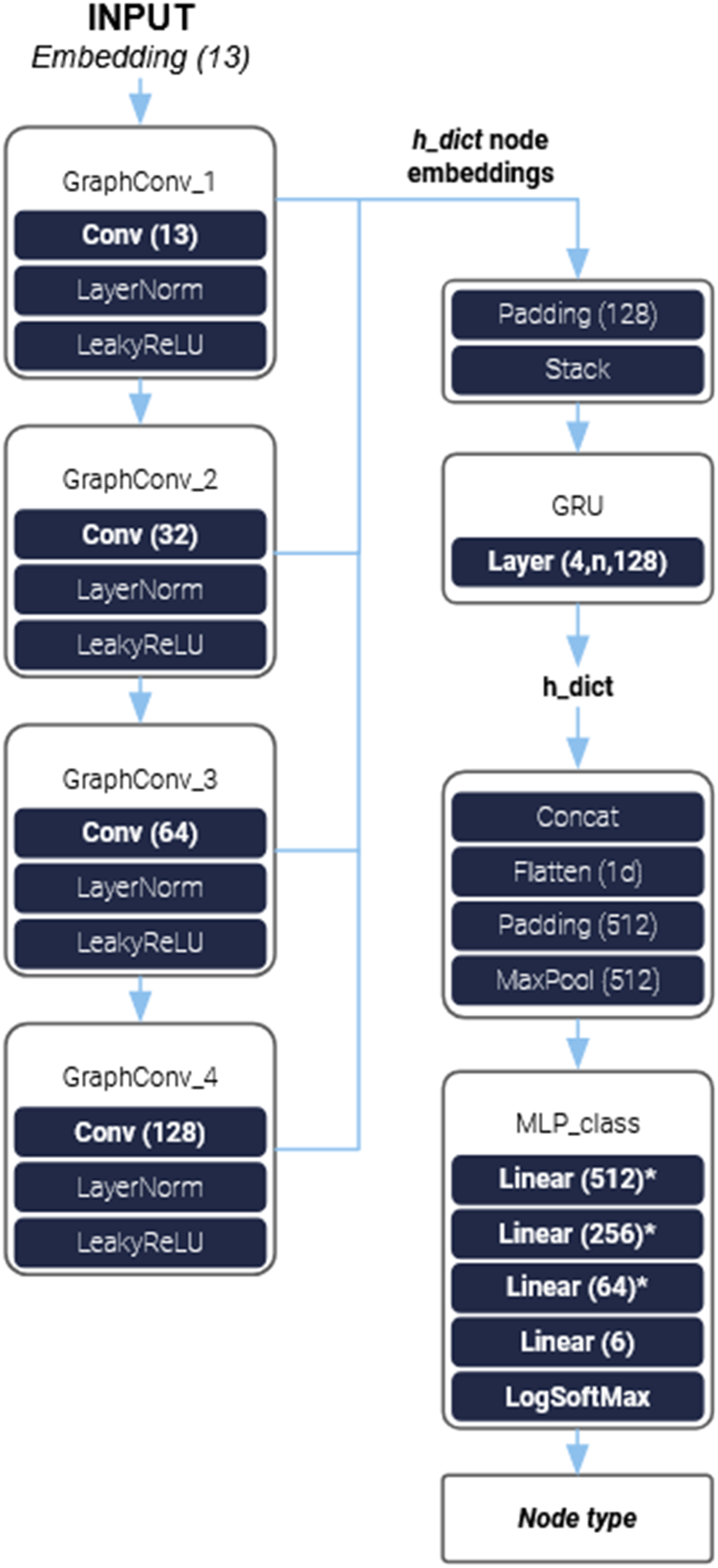

In our NN architecture, we also opted to implement a Gated Recurrent Unit (GRU)²⁷ that takes as an input the intermediate stacked node embeddings after each convolutional layer, in order to achieve a multi-level representation of the MP results. The change in performance can be seen in the chapter Application and Results.

We then concatenate and flatten the node embeddings into a 1D tensor that will function as the input for our multi-label classification MLP. The classification MLP uses Leaky ReLU as an activation function and has a final LogSoftMax activation. Alternatively, we also replaced the GRU with a simple pooling layer as well as only using the last node embedding representation from the convolution layers without the multi-level MP representation.

Regression models

The network architecture for regression problems resembles the classification network, consisting of a GNN followed by an MLP. Different from the multi-label classification network, we opted to use GAT (14) in the form of GATConv convolutional layers. The node embeddings of each attention head from the convolutional layers are then concatenated and flattened, and subsequently parsed to the MLP.

The MLP comprises multiple fully connected layers. In the final layer, the ground truth tensor representing the node type is concatenated with the intermediate tensor, resulting in an output of size 6, which represents the size of the node features to be predicted (Figure 2). For the co-pilot version with only angle and dimension prediction capabilities, we also concatenate the ground truth of the center point.

Figure 2.

NN architecture of regression model with GATConv and a final Sigmoid activation.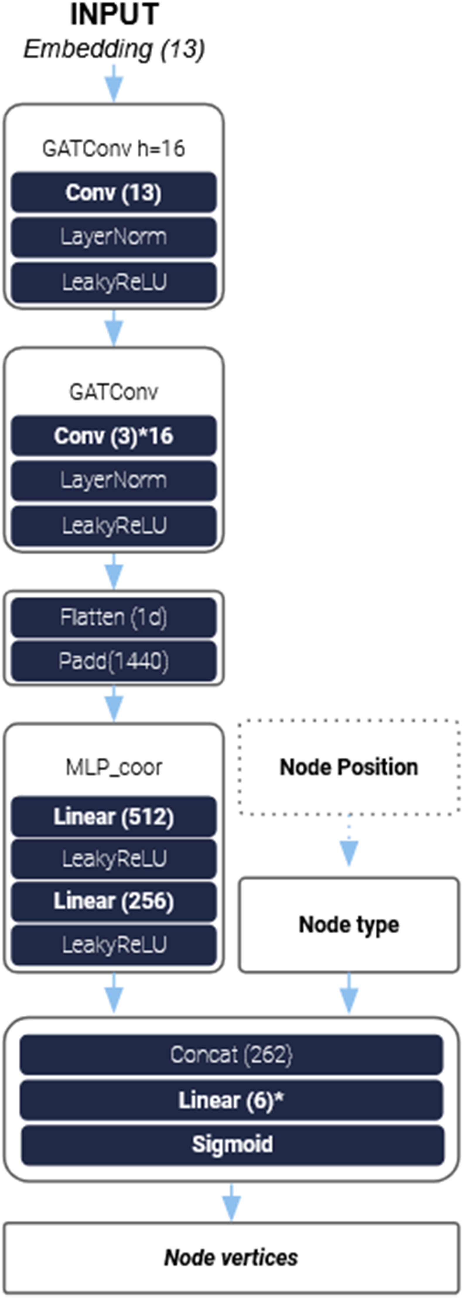

Training

Training the models required distinct hyperparameter configurations for the multi-label classification network and for the regression networks A) and B). These configurations are described separately.

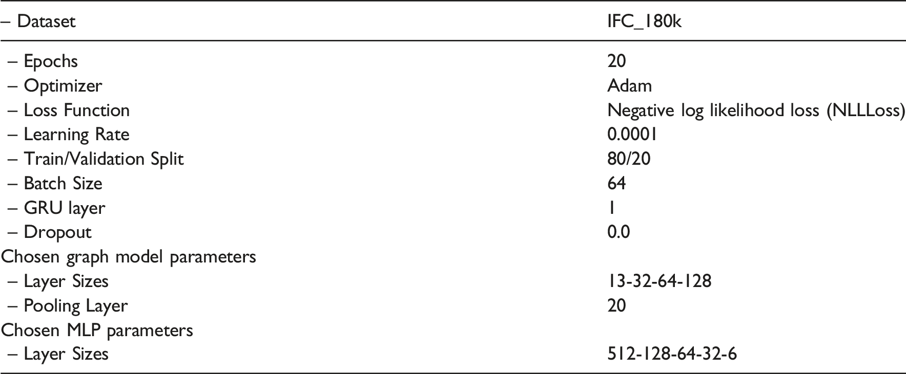
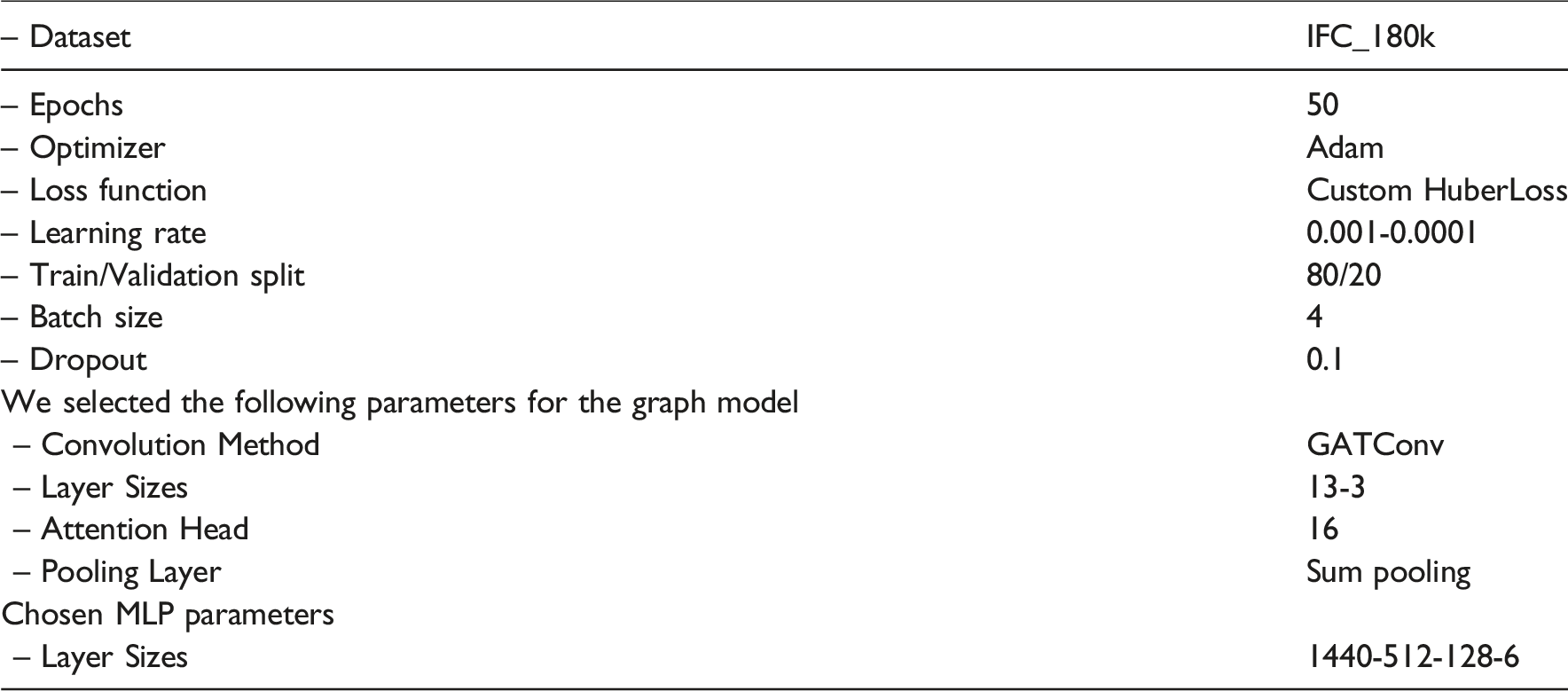
Model training was conducted using either an Nvidia RTX 3090 Ti or an Nvidia RTX A4000 on the IFC_180k dataset. When utilizing GNN, each epoch required approximately 3–4 h, whereas training without MP significantly reduced this time to 10–20 min, depending on the network parameters. To accelerate experimentation, a smaller dataset, IFC_18k, was employed for preliminary training trials before applying the optimized models to the full IFC_180k dataset with respect to the splitting method applied.

Given the high computational cost associated with training both networks, a systematic hyperparameter optimization was not feasible. Instead, a set of key parameters was selected based on empirical evaluation, allowing for iterative refinement toward the final network architecture.

Multi-label classification network

For the multi-label classification network, we chose following hyperparameters:

– Dataset	IFC_180k
– Epochs	20
– Optimizer	Adam
– Loss Function	Negative log likelihood loss (NLLLoss)
– Learning Rate	0.0001
– Train/Validation Split	80/20
– Batch Size	64
– GRU layer	1
– Dropout	0.0
Chosen graph model parameters
– Layer Sizes	13-32-64-128
– Pooling Layer	20
Chosen MLP parameters
– Layer Sizes	512-128-64-32-6

Regression network A

For both regression networks, we used regression-specific loss functions including MSE, RMSE, Chamfer distance, a custom Huber loss, and a vertex distance metric. IoU was considered, but was found to be unsuitable for systems with many degrees of freedom, where the predicted and ground truth components often do not overlap spatially, providing no information on spatial separation. For evaluation, we compute all pairwise Euclidean distances between the vertices of two oriented bounding boxes using torch. cdist, then take the mean of those distances. This provides a continuous, interpretable proximity score, even for disjoint geometries. The regression network model A) has the following hyperparameters:

– Dataset	IFC_180k
– Epochs	50
– Optimizer	Adam
– Loss function	Custom HuberLoss
– Learning rate	0.001-0.0001
– Train/Validation split	80/20
– Batch size	4
– Dropout	0.1
We selected the following parameters for the graph model
– Convolution Method	GATConv
– Layer Sizes	13-3
– Attention Head	16
– Pooling Layer	Sum pooling
Chosen MLP parameters
– Layer Sizes	1440-512-128-6

Regression network B

For the regression network B), we applied the same hyperparameter settings as for the regression network A).

Co-pilot

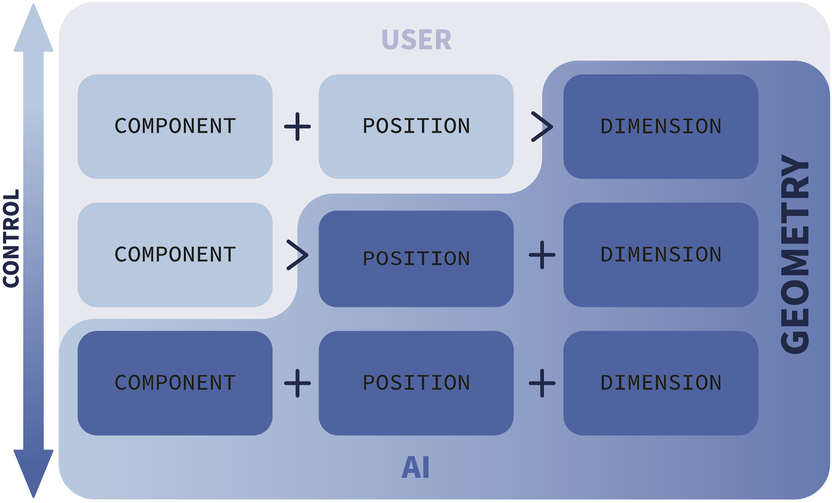
The co-pilot is designed to iteratively predict unique new elements based on a defined context, ensuring seamless integration into the user’s workflow while preserving the design intent. To achieve this, we propose three levels of human-AI interaction. These levels are based on user input and allow to determine the level of AI involvement according to the user’s preference, as illustrated in Figure 3:

1. Restricted Mode: The user specifies the component type and its exact position, while the co-pilot predicts only the dimensions of the geometry.

2. Partial Assistance Mode: The user provides only the component type, and the co-pilot predicts the placement, orientation (angle), and dimensions of the new component.

3. Fully Autonomous Mode: The co-pilot autonomously suggests the component type, position, orientation, and dimensions based on the local architectural context.

Figure 3.

Control levels of human-AI interaction, showing responsibility distribution.

Each of these modes corresponds to a distinct machine learning problem, requiring different neural network models tailored to the respective prediction tasks.

The co-pilot tool was developed within the commercial 3D computer graphics and computer-aided design application software Rhinoceros 3D (Rhino) based on prior experience with the software. We created a Rhino/Grasshopper script that allows fast and intuitive loading of trained models and automatic component prediction based on contextual information. However, the long-term objective for the tool is to operate platform-independently, assisting designers by providing context-based predictions.

The tool is implemented as a Hops component within Rhino’s algorithmic modeling plug-in Grasshopper, which runs a local host server to connect external scripts to Rhino’s native environment. The user has the ability to:

$•$ Input custom, random, or predefined building components.

$•$ Choose between three levels of human-AI interaction.

$•$ Execute the prediction process.

We propose an iterative workflow:

1. The user sketches a three-dimensional component, which is internally converted into a graph representation using a modified version of the algorithm employed for dataset creation.

2. The created graph serves as input for the neural network responsible for node type prediction and the subsequent network for feature prediction.

3. The predicted outputs, represented as tensors, are transformed back into three-dimensional geometry and visualized to the user.

4. The user can either accept the AI-generated suggestion or reject it.

The real-time interaction between the user and the AI model focuses on the objective that the final output remains aligned with the designer’s intent while informed from data-driven suggestions (Figure 4).

Figure 4.

Tool workflow explaining the interaction between the user and the neural networks in the backend.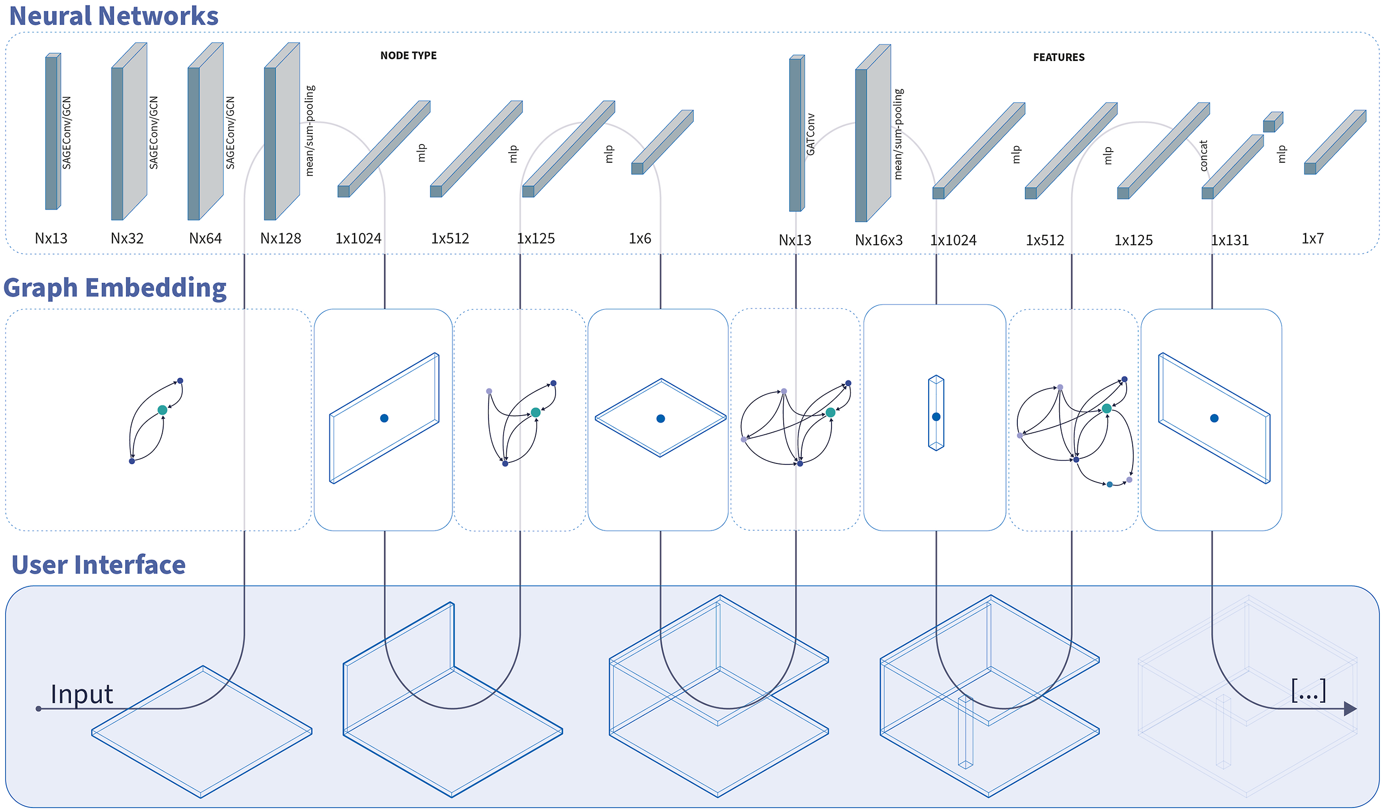

System Usability Scale

The System Usability Scale (SUS) is a widely adopted, cost-effective method for evaluating the usability of a system, product, or service within an industrial context.²⁸ It consists of a standardized questionnaire comprising (10) ten items, each rated on a five-point Likert scale to assess the degree of user agreement or disagreement.²⁹ The resulting SUS score ranges from 0 to 100 and is calculated using the following formula:

SUS = 2.5 (20 + \sum_{i = 1,3,5,7,9} ({SUS}_{i} - 1) - \sum_{i = 2,4,6,8,10} (5 - {SUS}_{i}))

(3)

where

{SUS}_{i}

represents the score for the

i

th item in the questionnaire.

The SUS provides a reliable measure of perceived usability, allowing for comparison across different systems and products. Higher scores indicate better usability, with specific interpretations such as a score of 71.4 considered ”Good” and 50.9 classified as ”OK”.²⁹

Application and results

In the following section we will show some of the results of our training and validation. The selected graphs and hyperparameters are not optimized, however they show a viable setting for training a context-informed co-pilot.

We want to acknowledge that the experimental setup in this work may introduce a certain degree of data leakage due to the nature of the data processing and augmentation technique employed. Specifically, the data augmentation technique of oversampling underrepresented classes (Figure 5). However, this does only happen in marginal cases depending on the deconstruction algorithm employed such as the IfcBuildingStorey element in the IFC_180k_hBFS dataset.

Figure 5.

Description of the dataset creation steps taken, including data augmentation, splitting and over- undersampling.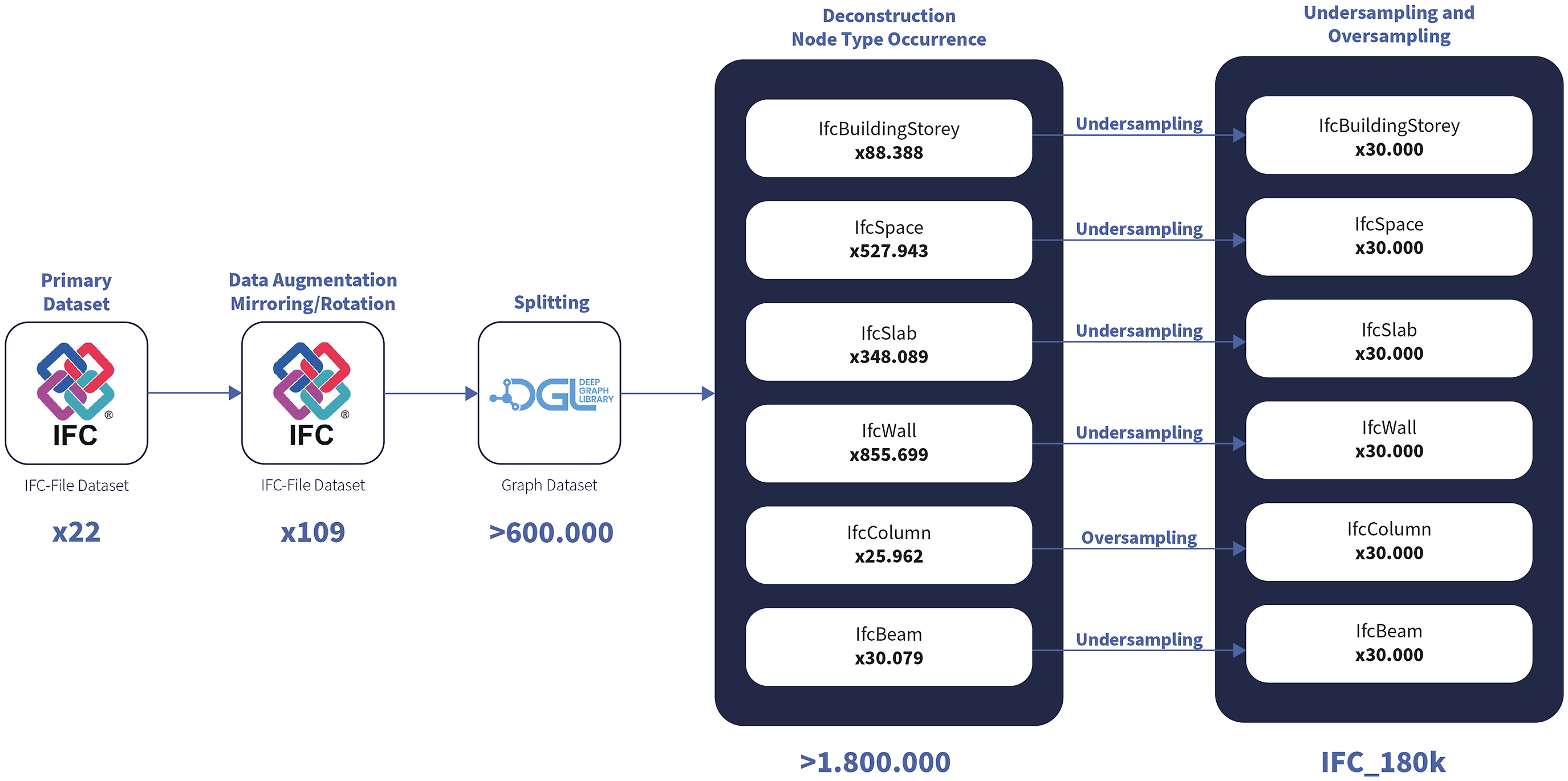

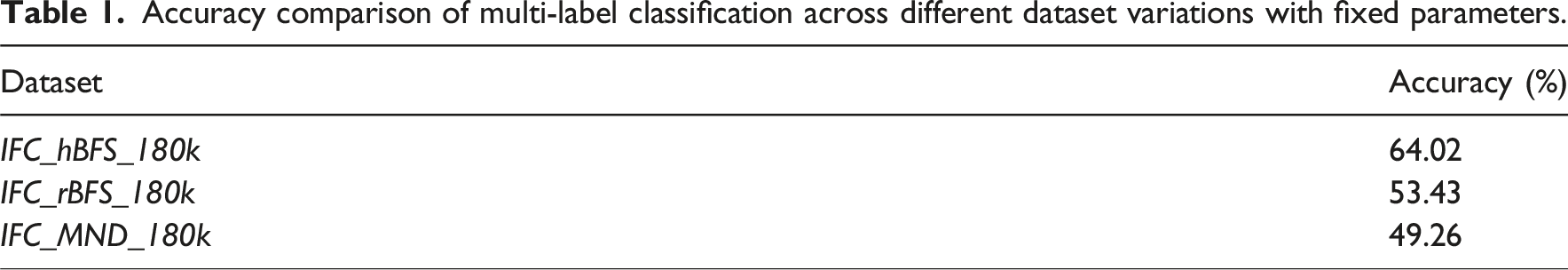
Across all three deconstructed datasets, the models exhibited superior performance when trained on the larger IFC_180k dataset compared to IFC_18k. Observations from the multi-label classification node type prediction task, applied to all models trained with identical parameters on the datasets (IFC_hBFS_180k, IFC_rBFS_180k, and IFC_MND_180k), indicate that IFC_hBFS_180k consistently outperforms the other two variants.

An example of the accuracy results for the dataset comparison, trained with fixed parameters over 45 epochs for the multi-label classification task, is shown in Table 1.

Table 1.

Accuracy comparison of multi-label classification across different dataset variations with fixed parameters.

Dataset	Accuracy (%)
IFC_hBFS_180k	64.02
IFC_rBFS_180k	53.43
IFC_MND_180k	49.26

Models results

The following results represent the highest-performing training outcomes for each model of the multi-label classification network and for the regression networks A) and B).

Multi-label classification network

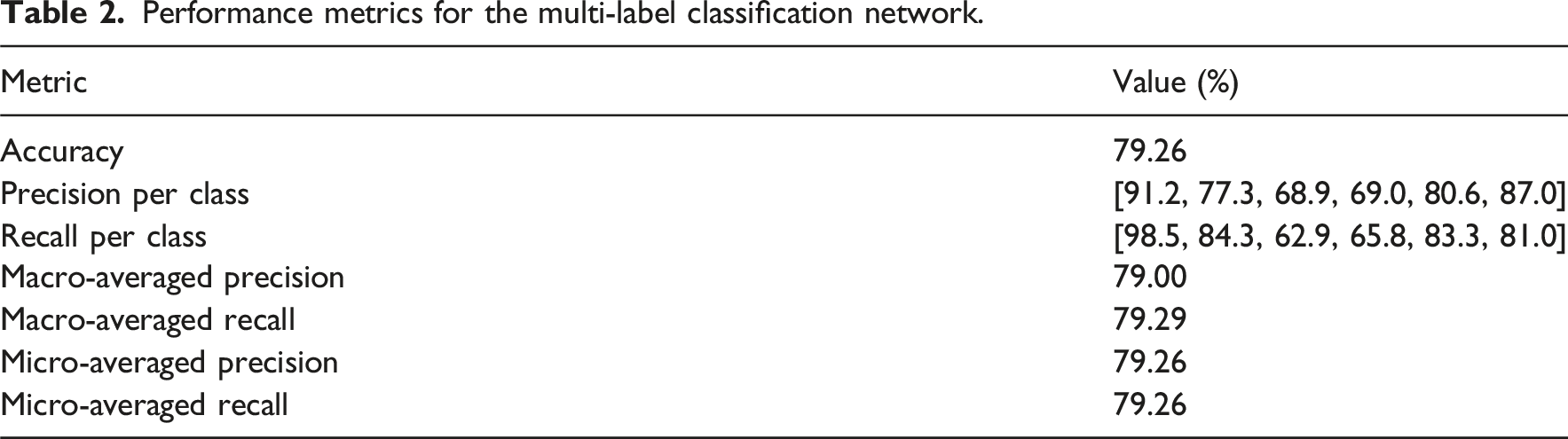
The final classification validation results indicate that, after 20 epochs (approximately 80 hours) of training with the specified settings on IFC_hBFS_180k, the network correctly predicts approximately 79% of the node types, with similar macro-averaged recall values (Table 2, Figure 6).

Table 2.

Performance metrics for the multi-label classification network.

Metric	Value (%)
Accuracy	79.26
Precision per class	[91.2, 77.3, 68.9, 69.0, 80.6, 87.0]
Recall per class	[98.5, 84.3, 62.9, 65.8, 83.3, 81.0]
Macro-averaged precision	79.00
Macro-averaged recall	79.29
Micro-averaged precision	79.26
Micro-averaged recall	79.26

Figure 6.

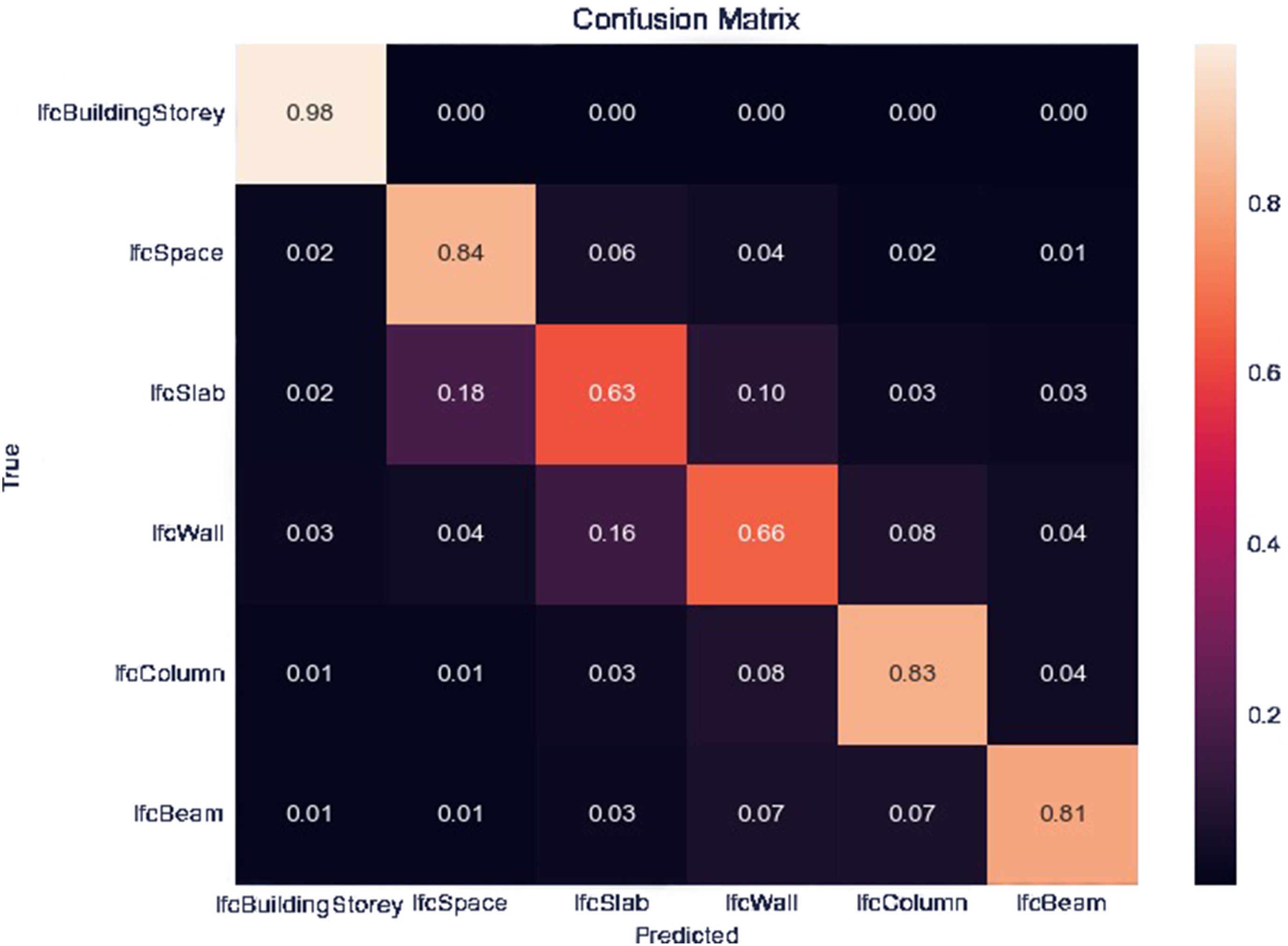
Confusion matrix illustrating the classification performance for different IFC elements.

The order of the predictions corresponds to IfcBuildingStorey, IfcSpace, IfcSlab, IfcWall, IfcColumn, and IfcBeam. Overall, the network demonstrated superior generalization when MP was enabled, utilizing a GRU and fewer hidden layers. Additionally, to prevent substantial divergence between training and validation loss, a dropout rate of 0.2 and 0.3 was utilized. The learning rate was fixed at 0.0001 throughout the training process.

In a multi-label classification problem with six outcomes, random guessing is analogous to a dice throw, yielding a statistical accuracy of $\frac{1}{6}$ or 16.67%. In contrast, our network achieves an accuracy of 79% based on the given context. The comparison highlights the efficacy of utilizing GNNs in non-deterministic environments with a given contextual information.

To further substantiate the above results, a similar network was trained without employing a GRU and omitting the MP of the GNN. These modifications produced the following multi-label classification MLP results after 20 epochs (approximately 3 hours):

– Accuracy	71.14%
– Precision per class	[85.4, 68,8, 63.2, 58.4, 73.3, 73.9]
– Recall per class	[91.7, 75.1, 52.3, 53.8, 74.4, 79.0]
– Macro-averaged precision	70.79%
– Macro-averaged recall	70.52%
– Micro-averaged precision	71.14%
– Micro-averaged recall	71.14%

The simple MLP model performs relatively well compared to random guessing. However, combining it with a graph model significantly improves its performance. In particular, a simple MLP network trains much faster than a GNN combined with a GRU. Due to the lack of parallelized batch training during our experiments, we relied on sequential mini-batch training, which resulted in slower training times. Consequently, a comparison of both approaches based on training time and computational power is not feasible under the given circumstances.

Regression network A

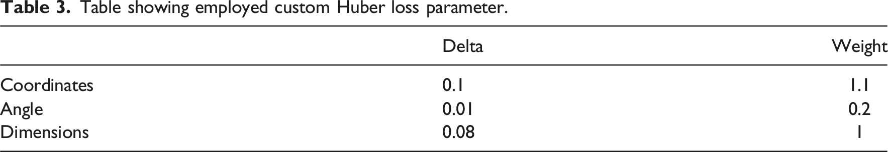
For regression network A), a custom Huber loss function was employed, incorporating varying weights and delta values for different tensor components.

The differentiation was implemented because each component contributes differently to the overall evaluation. For instance, a small deviation in coordinate prediction significantly impacts model performance, whereas an equivalent deviation in dimensional parameters has a comparatively lower effect.

During the training process, multiple Huber loss hyperparameter configurations were explored. Table 3 includes the most effective values identified through experimentation.

Table 3.

Table showing employed custom Huber loss parameter.

	Delta	Weight
Coordinates	0.1	1.1
Angle	0.01	0.2
Dimensions	0.08	1

We generally achieved good results with dropout rates of 0.0, 0.1, and 0.2, and a stepped learning rate adjustment every 8 to 10 epochs.

The evaluation reveals that models with varying hyperparameter settings converged at an average distance evaluation of approximately 22 meters over the entire dataset (Figure 7).

Figure 7.

Regression A) results. (a) Training and Validation Loss versus Epochs. (b) Training and Validation Evaluation versus Epochs.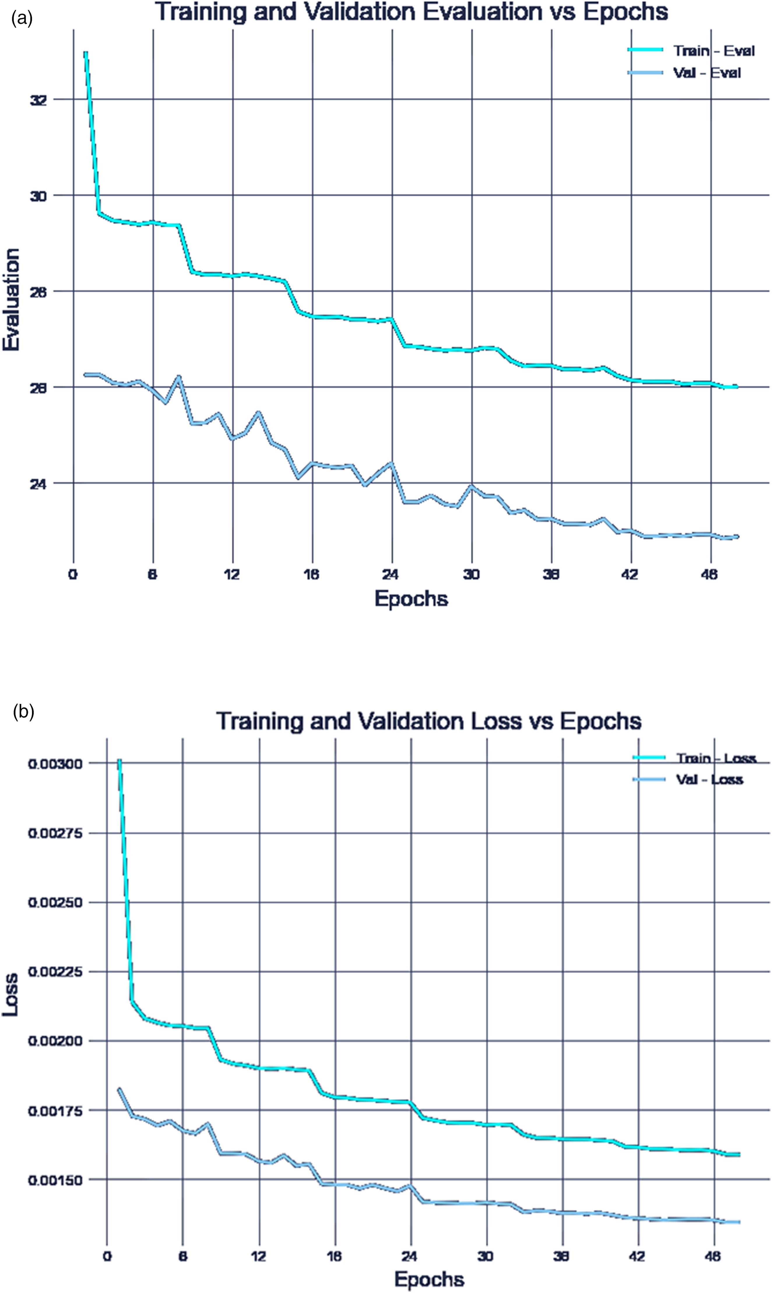

Regression network B

For the regression model B) we employed similar hyperparameters as for the regression model A). Since the coordinates are concatenated with the node type and entered into the MLP before the final activation layer, the features to predict are only the angle and dimensions, resulting in an output size of 4. Given that the coordinates are known, model B) performs significantly better than model A), converging at approximately 15 meters (Figure 8).

Figure 8.

Regression B) results. (a) Training and Validation Loss versus Epochs. (b) Training and Validation Evaluation versus Epochs.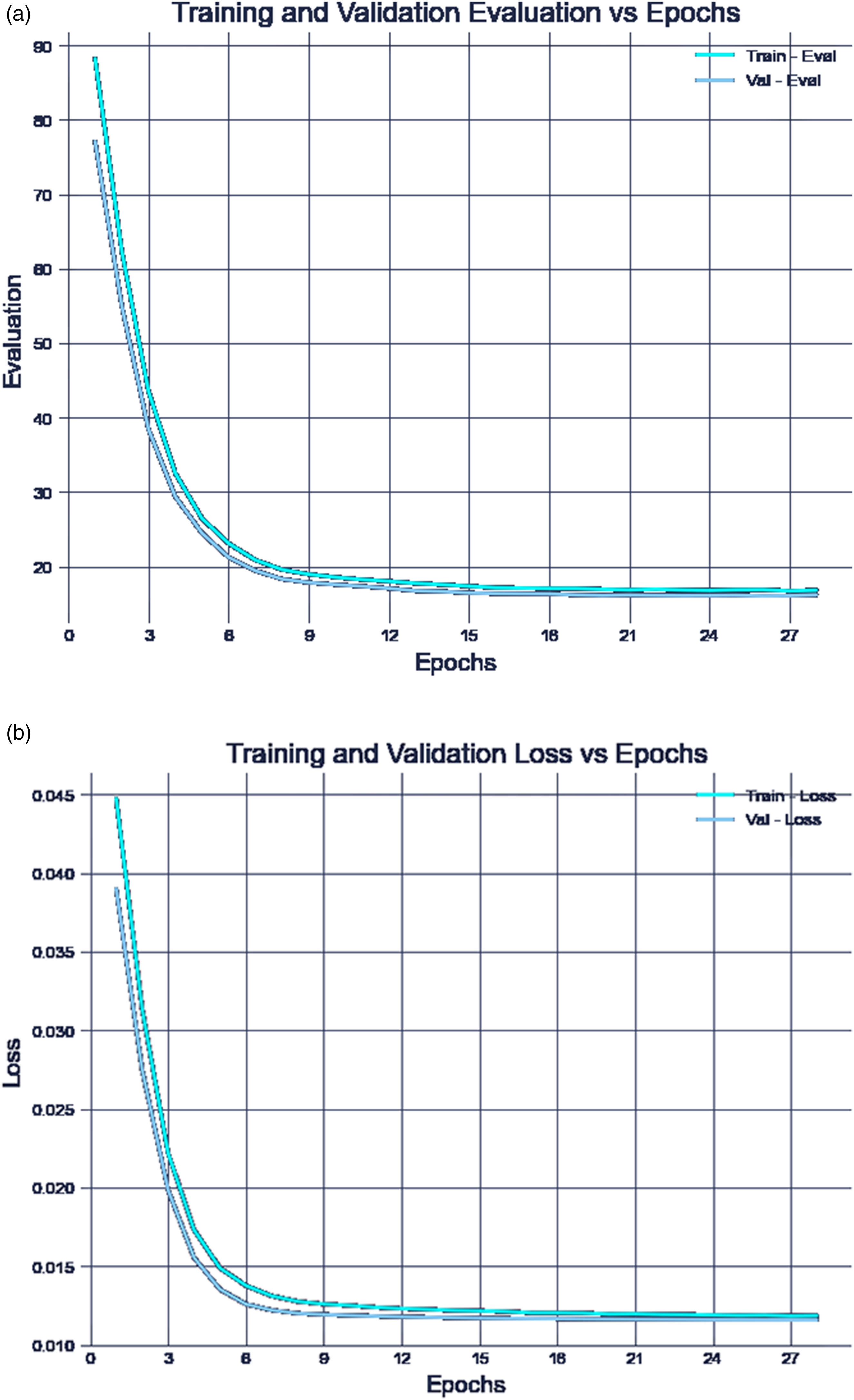

The learning performance of our NN reflects its ability to extract complex graph patterns, enabling the prediction of node types, positions and dimensions that approximate the ground truth. However, architectural quality cannot be evaluated by technical metrics alone.

Qualitative evaluation

To assess practical reliability and design adequacy, we conducted a qualitative evaluation to highlight possible areas where spatial accuracy remains insufficient for real-world applications. For this purpose, we conducted a SUS survey with 20 participants, 19 of them were architecture students (13 bachelor, 6 master). Among them, 55% were familiar with the concept of BIM, while 60% had intermediate experience with Rhino, and only 20% reported that they possessed “good skills” in Grasshopper.

The task for the participants was to continue working on various simplified and incomplete 3D buildings in Rhino using the co-pilot tool.

As shown in Figure 9, the Restricted Mode achieved the best overall SUS score with 56.25, followed by Fully Autonomous Mode with 53.75, and finally Partial Assistance Mode with 51.875, all indicating ”OK” results.

Figure 9.

System Usability Scale results for three different control modes from 20 participants.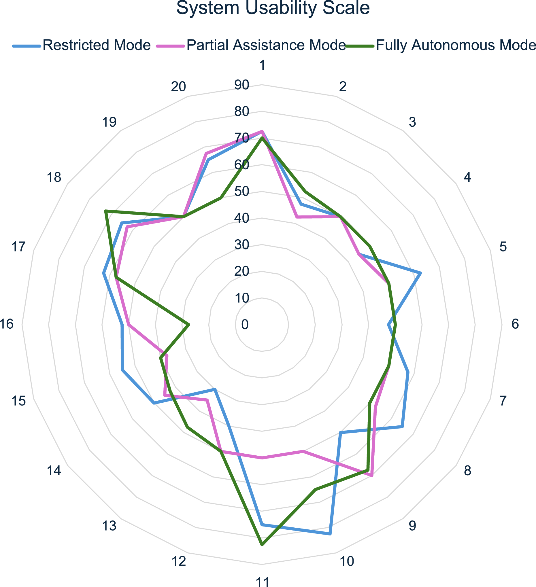

According to respondent feedback, the Restricted Mode received the highest SUS score, largely due to its convenient ability to adjust geometric placement by aligning the center of the suggested building element with the user’s intent.

However, this mode requires the most preset configurations and mouse clicks to generate initial suggestions, making it more time-consuming. Despite the effort, all participants were able to successfully complete their tasks in this mode, although some inconsistencies in orientation and proportions were noted in strictly orthogonal assemblies (Figure 10(a)).

Figure 10.

Illustrative examples of visual performances. (a) Restricted Mode. (b) Partial Assistance Mode. (c) Fully Autonomous Mode.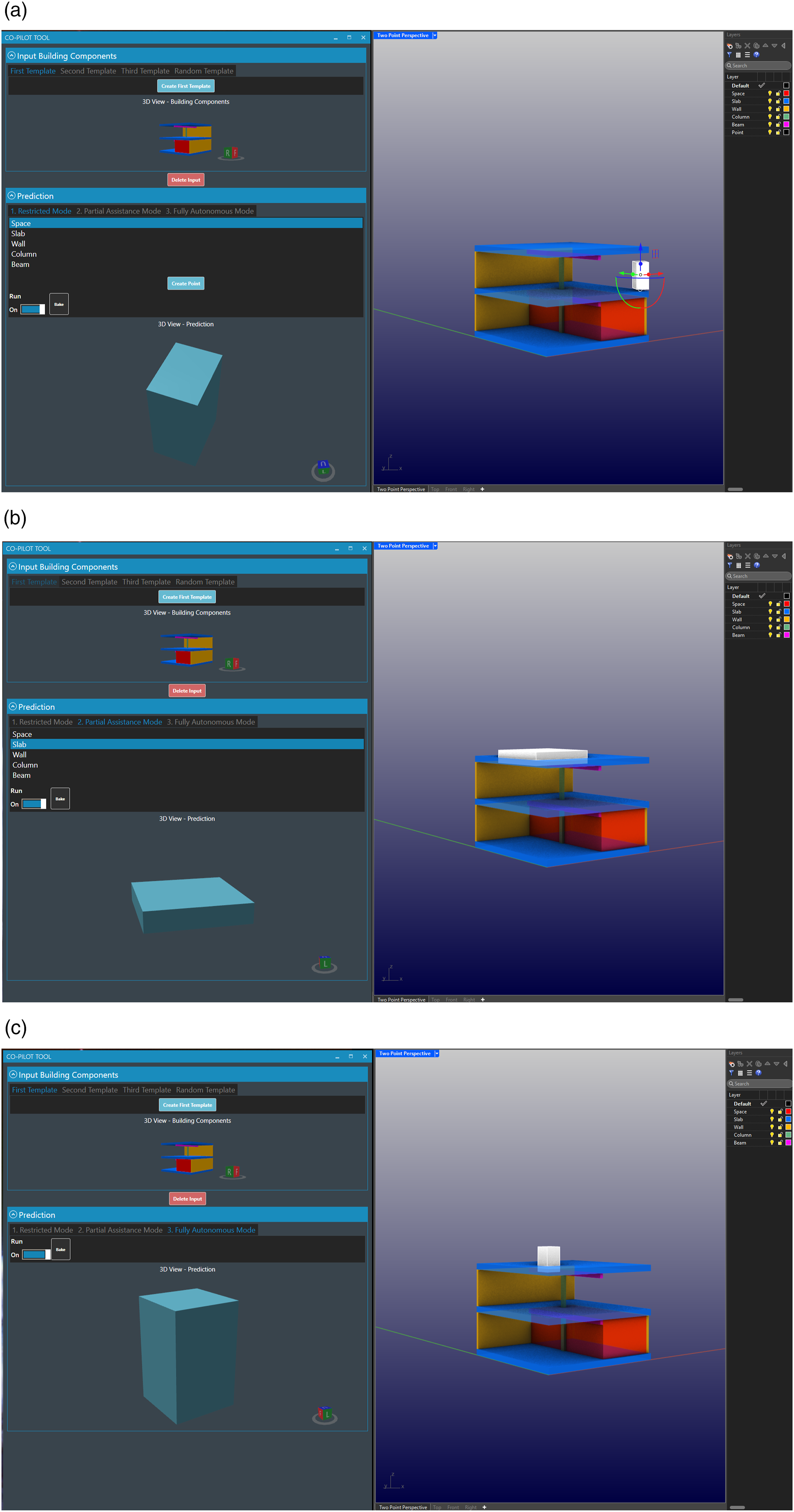

The Partial Assistance Mode (Figure 10(b)) allows users to choose between component types and offers a broader variety of suggestions across different building components compared to the Fully Autonomous Mode (Figure 10(c)). However, participants using both the Partial Assistance Mode and Fully Autonomous Mode struggled to complete tasks due to overly simplistic predictions, which often required significant user intervention to adapt and complete.

While the tool assists in the generation of building elements, it was observed that task completion in Fully Autonomous Mode and Partial Assistance Mode often relied on user corrections, especially when AI predictions were inaccurate. These findings suggest that the AI component of the tool is still limited in its ability to autonomously handle more complex design scenarios, with much of the success being driven by user input. In contrast, the Restricted Mode demonstrated a more balanced interaction between AI suggestions and user control, which helped to improve task completion despite requiring more manual configuration.

In terms of overall efficiency and decision-making, the impact of the tool on workflows optimization requires further investigation. While Restricted Mode facilitated certain tasks by enabling geometric placement adjustments, further studies are needed to determine whether the tool can fully replace or enhance traditional manual workflows in the long term.

The regression model A) shows predictions that are constrained to a narrow range of geometric locations, as observed visually. Overgeneralization can be caused by several potential factors, including insufficient training data, incorrect normalization or scaling, or an inappropriate loss function, etc.

To address the issue of reduced output variability, several regularization techniques can be employed to prevent the model from becoming overly complex and to closely fit the training data.³⁰ These techniques include $L 1$ and $L 2$ regularization methods, cross-validation, early stopping, and data augmentation.

In general, a more systematic and design-oriented evaluation is needed to better characterize model behavior and guide future improvements of architectural ML.

Conclusion and discussion

By overcoming the limitations of pixel- and voxel-based AI approaches and building on the advantages of GNNs in architecture, this study presents a viable generative AI methodology for context-informed autocompletion co-pilots. Additionally, it exemplifies a viable use of DGMG and highlights the potential of using heterogeneous graphs for architectural purposes capable of learning spatial and relational patterns in 3D space. The study identifies several challenges to address:

1. Availability and Standardization of 3D Building Datasets: A key limitation of this study lies in the lack of access to a structurally and typologically diverse IFC dataset. Despite using real-world BIM data, the final dataset is restricted to residential projects from a narrow regional and functional context. This constraint limits the generalization of our findings across broader architectural domains. Additionally, inconsistencies in modeling practices across firms introduce noise that complicates data preprocessing and standardization. These factors underscore the need for more robust, open-access IFC datasets that span a variety of building types, spatial organizations, and geometric complexities. Future research should focus on curating such datasets and conducting quantitative and qualitative analyses of variability in building function, layout, and form to support more definitive claims about model generalization and real-world applicability.

2. Evaluation Metrics and Usability of the Tool: The absence of qualitative and objective architectural evaluation metrics remains a limitation. While the co-pilot can be assessed using functional criteria, for instance, evaluating the accuracy of a proposed load-bearing column based on its predicted dimensions, material, and placement through structural integrity calculations, broader architectural assessment methods are required. The usability testing of the co-pilot yielded ”OK” results, indicating that there is room for improvement, particularly in refining human-machine interaction. Additionally, increasing the sample size would enhance the representativeness of the findings. Notably, the higher acceptance of the Restricted Mode, where users retain greater decision-making authority compared to the AI, underscores the importance of maintaining a balanced approach between automation and user control.

3. Geometric Predictions and Logical Constraints: While the AI-driven prediction of architectural geometry exhibits a high degree of flexibility, it could benefit from additional logical constraints. For example, implementing structural rules, such as ensuring that columns are correctly attached to slabs or that one column is properly aligned over another, could enhance the functional reliability of the generated designs. Furthermore, improving the proportions of predicted geometries would contribute to more architecturally sound and structurally coherent outcomes.

4. Dataset Composition and Generalization Bias: While each subgraph is unique and the datasets were cleanly partitioned at the subgraph level, this setup may introduce distributional bias, as recurring local patterns within individual models could affect generalization. Using entirely unseen IFC models for evaluation would provide a more robust assessment of the model’s ability to generalize to new design contexts.

We consider graphs to be a versatile and effective methodology for lightweight 3D architectural representation and ML applications in the built environment. While this study focuses on a co-pilot for building autocompletion, it constitutes an initial step toward a more comprehensive foundation model for architectural design.

Our findings suggest that the co-pilot has the potential not only to generate architectural elements but also to provide additional insights, such as material suggestions, cost estimations, and qualitative architectural features. Furthermore, its applicability could extend beyond architecture to domains such as Mechanical, Electrical, and Plumbing (MEP) design, where automated component placement and optimization may improve efficiency.

Future developments of the tool could integrate functionalities including classification tasks, generative autocompletion, retrieval-augmented generation, and advanced design assistance. These features may support dynamic design iterations, code compliance verification, on-site sensor and image data evaluation, sustainable material recommendations, and automated detailing of component connections. While the current approach demonstrates promising potential, further research and iterative refinements are required to fully realize its capabilities and ensure its effective integration into architectural and engineering workflows.

Footnotes

Declaration of conflicting interests

The author(s) declared no potential conflicts of interest with respect to the research, authorship, and/or publication of this article.

Funding

The author(s) disclosed receipt of the following financial support for the research, authorship, and/or publication of this article: This work was supported by the Deutsche Forschungsgemeinschaft (EXC 2120/1 – 390831618), Horizon Europe under grant agreement numbers 101189678 and 101189678 (AMALTEA), and Zukunft Bau (10.08.18.7-22.45). Views and opinions expressed are, however, those of the author(s) only and do not necessarily reflect those of the European Union. Neither the European Union nor the granting authority can be held responsible for them.

ORCID iDs

Markus Renner

Diellza Elshani

Matthias Hornung

Thomas Wortmann

References

Büchel

Jan

Engels

Barbara

. Digitalisierung der Wirtschaft in Deutschland, 2021. Retrieved from. https://www.bmwk.de/Redaktion/DE/Publikationen/Digitalisierungsindex/publikation-download-Langfassung-digitalisierungsindex-2021.html

Zawada

Rybak-Niedziółka

Donderewicz

, et al. Digitization of AEC industries based on BIM and 4.0 technologies. Buildings 2024; 14(5): 1350. https://www.mdpi.com/2075-5309/14/5/1350

Izbash

Babayev

. Digital evolution in AEC industry: bridging BIM, building codes, and future technologies. IOP Conf Ser Earth Environ Sci 2024; 1376(1): 012004.

Lehmann

Buschek

. Examining autocompletion as a basic concept for interaction with generative AI. com 2021; 19(3): 251–264.

Vaswani

. Attention is all you need. Adv Neural Inf Process Syst 2017; 1: 03762.

Izadi

Katzy

van Dam

, et al. Language models for code completion: a practical evaluation. In: Proceedings of the 46th International Conference on Software Engineering (ICSE), April, Lisbon, Portugal. New York, NY: Association for Computing Machinery, 2024.

Jang

Lee

. Interactive design by integrating a large pre-trained language model and building information modeling, 2023. https://arxiv.org/abs/2306.14165

Reformat

D’Aniello

Gaeta

. Knowledge graphs, category theory and signatures. In: Proceedings of the 2018 IEEE/WIC/ACM International Conference on Web Intelligence (WI). Piscataway: IEEE, 2018, pp. 480–487.

Scarselli

Gori

Tsoi

, et al. The graph neural network model. TsoiIEEE Trans Neural Network 2008; 20: 61–80.

10.

Elshani

Lombardi

Fisher

, et al. Knowledge graphs for multidisciplinary Co-design: introducing RDF to BHoM. In: Proceedings of LDAC@ ESWC, Hersonissos, Greece, May 29, 2022, pp. 32–42.

11.

Zhang

Song

Huang

, et al. Heterogeneous graph neural network. In: Proceedings of the 25th ACM SIGKDD International Conference on Knowledge Discovery & Data Mining (KDD ’19). : Association for Computing Machinery, 2019, pp. 793–803.

12.

Pan

Chen

, et al. A comprehensive survey on graph neural networks. CoRR, abs/1901.00596 2019, Retrieved from. https://arxiv.org/abs/1901.00596

13.

Vinyals

Dyer

, et al. Learning Deep generative models of graphs. CoRR 2018; 18: 03324, Retrieved from. https://arxiv.org/abs/1803.03324

14.

Veličković

Cucurull

Casanova

, et al. Graph attention networks, 2017, Retrieved from https://arxiv.org/abs/1710.10903

15.

Wang

Shi

, et al. A survey on heterogeneous graph embedding: methods, techniques, applications and sources. IEEE Trans Big Data 2023; 9(2): 415–436.

16.

Tang

Shao

Sebe

, et al. Graph transformer GANs with graph masked modeling for architectural layout generation, 2024. Retrieved from: https://arxiv.org/abs/2401.07721

17.

Nauata

Hosseini

Chang

K-H

, et al. House-gan++: generative adversarial layout refinement network towards intelligent computational agent for professional architects. In: Proceedings of the IEEE/CVF Conference on Computer Vision and Pattern Recognition. Piscataway: IEEE, 2021, pp. 13632–13641.

18.

Nauata

Chang

K-H

Cheng

C-Y

, et al. House-GAN: relational generative adversarial networks for graph-constrained house layout generation. CoRR, abs/2003 2020; 16: 06988, Retrieved from. https://arxiv.org/abs/2003.06988

19.

Huang

Tang

, et al. House-GAN: relational generative adversarial networks for graph-constrained house layout generation. Graph2Plan: learning floorplan generation from layout graphs. ACM Trans Graph 2020; 39(4): 3392391.

20.

Zhong

Koh

Fricker

. Building-GNN: exploring a co-design framework for generating controllable 3D building prototypes by graph and recurrent neural networks. In: Proceedings of the International Conference on Education and Research in Computer Aided Architectural Design in Europe (eCAADe). Belgium: eCAADe, 2023, pp. 431–440.

21.

Chang

K-H

Cheng

C-Y

Luo

, et al. Building-GAN: graph-conditioned architectural volumetric design generation. In: Proceedings of the IEEE/CVF international conference on computer vision. Piscataway: IEEE, 2021, pp. 11956–11965.

22.

Guerrero

, et al. SStructureNet: hierarchical graph networks for 3D shape generation, 2019. Retrieved from: https://arxiv.org/abs/1908.00575

23.

Bauscher

Dai

Elshani

, et al. Learning and generating spatial concepts of modernist architecture via graph machine learning. CAADRIA 2024; 14: 106129.

24.

Hamilton

Ying

Leskovec

. Inductive representation learning on large graphs. Adv Neural Inf Process Syst 2017; 30: 02216.

25.

Kipf

Welling

. Semi-supervised classification with graph convolutional networks. Retrieved from 2016. https://arxiv.org/abs/1609.02907

26.

Schlichtkrull

Kipf

Bloem

, et al. Modeling relational data with graph convolutional networks. In: The semantic web: 15th international conference, ESWC 2018, Heraklion, Crete, Greece, June 3–7, 2018, proceedings 15, 2018, pp. 593–607.

27.

Cho

. On the properties of neural machine translation: encoder-decoder approaches, 2014. Retrieved from. https://arxiv.org/abs/1409.1259

28.

Brooke

others . SUS-A quick and dirty usability scale. Usability evaluation in industry 1996; 189(194): 4–7.

29.

Lewis

. The system usability scale: past, present, and future. Int J Hum Comput Interact 2018; 34(7): 577–590.

30.

Park

Chang

, et al. Gradient-coherent strong regularization for Deep neural networks. CoRR, abs/1811 2018; 18: 08056, Retrieved from: https://arxiv.org/abs/1811.08056

31.

Liang

Zhong

Koh

. Building-VGAE Generating 3D detailing and layered building models from simple geometry. Proceedings of eCAADe 2024. Belgium: eCAADe, 2024.

32.

Altieri

Alex

. The impacts of BIM on the AEC industry. Columbia: Newsroom, Vectorworks, Inc, 2024. https://www.vectorworks.net/en-US/newsroom/bim-in-the-aec-industry?utm_source=chatgpt.com

Training and evaluating a Co-pilot tool using graph neural networks for generating non-orthogonal building typologies in architectural autocompletion

Abstract

Keywords

Introduction

AI-driven design assistance

Graph-based representation and GNN

Research gaps and problem statement

Methodology

Data preparation and embedding techniques

Models

Multi-label classification model

Regression models

Training

Multi-label classification network

Regression network A

Regression network B

Co-pilot

System Usability Scale

Application and results

Models results

Multi-label classification network

Regression network A

Regression network B

Qualitative evaluation

Conclusion and discussion

Footnotes

Declaration of conflicting interests

Funding

ORCID iDs

References